Modeling of Environmental Systems

Transcription

1 Modeling of Environmental Systems The next portion of this course will examine the balance / flows / cycling of three quantities that are present in ecosystems: Energy Water Nutrients We will look at each of these at two scales: Global Ecosystem Before we can build models of these phenomena, we need to have some background on the functioning of these systems with respect to these quantities

2 Water Budget Equations Assuming we can bound a terrestrial ecosystem, and further assume that it is in a steady state over the period we wish to study it, we can come up with the following water budget: dv dt = 0 = p + si + gi - so go - et where: p is precipitation si is surface water inflow gi is groundwater inflow so is surface water outflow go is groundwater outflow (all quantities averaged over the period) Recalling groundwater s long residence time, we can take the difference between groundwater terms to be negligible, and since water flows from land to ocean, we will remove the si term

3 Water Budget Equations This leaves us with the following equation: dv = 0 = p -so-et or dt p = so + et Hornberger et al Elements of Physical Hydrology. The Johns Hopkins University Press, Baltimore and London.

4 Water Flow Processes Up Close Taking a closer look, we can identify a few more processes: Precipitation Transpiration Evaporation Throughfall Stemflow Groundwater Soil Water Uptake Drainage Runoff p = so + et We will focus on how the uptake and transpiration processes work Soil water is drawn up through the plant root systems, moves through the plant, and is expelled from the plant leaves as transpiration into the atmosphere. How and why does this happen?

5 The Concept of Water Potential The reason is because there is a constant gradient of water potential (from soil to root to xylem to leaf to atmosphere), and this potential gradient is constantly dragging the water up and out Water potential is the free energy of water, measured in units of pressure (the commonly used SI unit is Megapascales [Mpa]) Pure water in liquid form at 20 o C and 1 atmospheric pressure (e.g. distilled water sitting in an unenclosed basin at sea level) has zero water potential In terrestrial ecosystems, the water in the stocks is reduced in concentration when compared with pure liquid water, thus water potentials are negative

6 Water Potential vs. Relative Humidity Salisbury, FB and C. Ross Plant Physiology. Wadsworth, Belmont, CA. An unsaturated atmosphere has a large water potential

7 Soil Water Potential Although the gradient that will draw water from the soil to the atmosphere (via plants) is usually present, there are counteracting forces along the way as well The water in soil is held to the soil particles as thin film of water, against the pull of gravity The thicker the film, the less tightly the water at the outer rim is held and the more easily it can be taken by plants This attractive force between water and surfaces is called matric potential The total amount of water a soil can hold per unit soil volume is a function of the surface area of all the particles within that volume and the amount of air space present between these particles, and varies by soil type

8 Soil Water Potential Soil matric potentials that are less negative than approximately Mpa are too weak to retain water against gravity Soil water content at this point is called the field capacity As soils dry, and these films become thinner, the remaining water is held more tightly and the matric potential becomes more negative Many plants cannot extract water from soils with matric potentials that are more negative than approximately 1.5 Mpa This condition is called the permanent wilting point Soils are a mixture of particles of various sizes, so a soil s aggregate performance is a function of the mixture

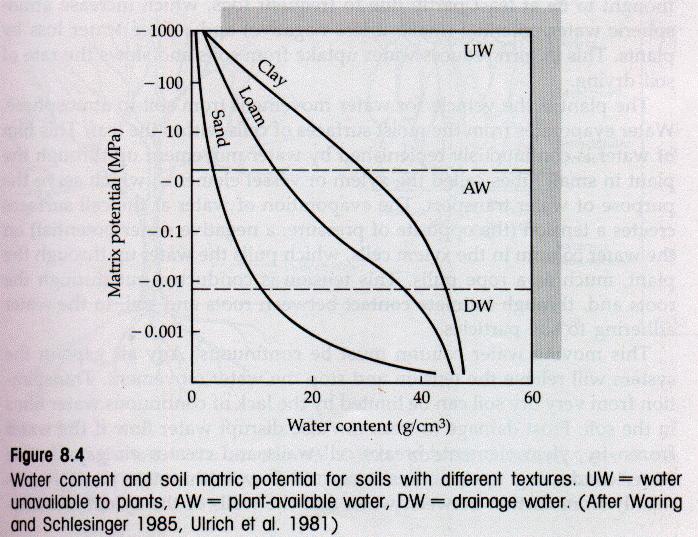
9 Soil Water Potential

10 Water Movement through the Soil-Plant-Atmosphere Continuum Soil water that can be freed from the soil can proceed to the atmosphere in two ways: Evaporation - Water in the soil evaporates directly into the atmosphere. Evaporation only affects the thin surface layer of soils, as the resistance to liquid water movement in soils is high Transpiration - Plants provide an ideal conduit for the movement of water between soils and the atmosphere. Roots grow deep into the soil and can tap into water reserves far from the surface, providing a pathway between the deeper soil and the atmosphere

11 Water Movement through the Soil-Plant-Atmosphere Continuum The movement of water from the soil through plant and into the atmosphere is controlled by stomata, tiny holes on the back of leaves The atmosphere is usually drier than the air inside the stomata, thus there exists a water potential gradient (the potential in the outside air is more negative) causing the water move from the stomata into the atmosphere

12 Water Movement through the Soil-Plant-Atmosphere Continuum The negative water potential in the atmosphere is transferred to a continuous column of liquid water that begins in the root and ends in the leaf The tissue that the water passes through is called xylem, which provides an uninterrupted pathway for water movement The tension is conducted out through the roots, and through contact between roots and soil, to the water adhering to soil particles This water column must be continuous. Any air gaps in the system will relieve the tension and stop the movement of water. Root surfaces must be in direct contact with the soil water film

13 Water Movement through the Soil-Plant-Atmosphere Continuum The actual rate of flow of water up through the plant, and thus from the soil to the atmosphere is a function of the differences in water potential between these two ends of the gradient and the resistance to the flow Resistance within the plant results mainly from friction between water and the walls of the xylem elements through which it passes The force of gravity also works against the rate of water movement up the stem During times of water stress, the guard cells lose water, reducing the turgor of the cells. As the guard cell loses turgor, the stomata will close, to further reduce the loss of water

14 Models of Potential Evapotranspiration While we have described the physical mechanisms that controls transpiration, we have not dealt with the biological complexity associated with when plants open or close their stomata As living things, plants respond to water (and other stresses) in a complex fashion, and while we can model this behavior as a function of many factors, these are very complex models that often still require calibration We can simplify a little by modeling potential evapotranspiration; the amount of water that would evaporate and transpirate under optimal conditions (i.e. given a certain amount of water and energy, what is the maximum amount that could evapotranspirate?)

15 Models of Potential Evapotranspiration Naturally to model evapotranspiration in Stella, we need to be able to express how it occurs mathematically, as a function of a set of quantities we can measure or calculate. Here are four methods of doing this: 1. The Thornthwaite Evaporation Equation (usually operated on a monthly basis) 2. The Dalton Evaporation Law (just evaporation, excluding the action of plants) 3. The Penman-Monteith Equation (adds plants) 4. Making use of the Bowen Ratio / Energy Balance (requiring detailed information about the energy balance)

16 1. The Thornthwaite Evaporation Equation The Thornthwaite Evaporation Equation is an empirical equation to estimate PET: 12 10Ti E p = k 1.6 i= 1 T where T i is monthly mean air temperature T is calculated using the following equation: ( ) 514 T = 0.2T i k is an empirical parameter related to latitude Works best at mid-latitudes and must be applied monthly i= 1 A

17 2. The Dalton Evaporation Law The Dalton Evaporation Law expresses the drying power of the air, somewhat abstractly: E a = f(u)(e 0 -e a ) where: E a is the PET for an extended wet surface e 0 is the saturation vapor pressure of the surface, which is a function of surface temperature e a is the actual vapor pressure of the air at the same height f(u) is a function of windspeed at a given height This can be applied over any time period, but requires surface temperature data, and the windspeed function must be represented accurately

18 3. The Penman-Monteith Equation The Penman-Monteith Equation builds on Dalton s ideas, including more physically-based factors: where: R n is net radiation G is soil heat flux ρ a is the mean air density at constant pressure c p is the specific heat of the air (e s -e a ) is the vapor pressure deficit r a is aerodynamic resistance is the slope of the sat. vapor pressure temp. relationship γ is the psychrometric constant is the bulk resistance, which includes stomatal action r s Energy input Aerodynamics Plant physiology

19 4. Bowen Ratio / Energy Balance You can calculate the ratio between sensible and latent heat fluxes, and this is known as the Bowen Ratio (β): β = H / LE The sensible heat flux is often difficult to measure, but if you can estimate the Bowen Ratio, you can rewrite the net radiation balance equation in terms of latent heat: R n = H + LE + G R n = (β * LE) + LE + G LE = (R n - G) / (1 + β) We can convert the latent heat to potential evapotranspiration based on the latent heat of vaporization (the amount of energy required to convert liquid water to vapor, 2.45*10 6 J/kg at 20 degrees C)

20 Modeling Ecosystem Water and Energy Energy-Water-Interaction ~ reflectance ~ LAI wilting point ~ insolation transmission absorption K field capacipty Transpiration evaporation water in soil water run off field capacipty ~ ppt We will model transpiration, as a function of available energy and water, using the latent heat of vaporization: Transpiration = 0.7*absorption*((soil water wilting point)/(field capacity wilting point))/