AN ECONOMIC ANALYSIS OF SCRAPPAGE ROBERT W. HAHN

Transcription

1 AN ECONOMIC ANALYSIS OF SCRAPPAGE ROBERT W. HAHN SEPTEMBER 1993

2 An Economic Analysis of Scrappage* Robert W. Hahn American Enterprise Institute th Street, N.W. Suite 1100 Washington, D.C December 1993 *Mr. Hahn. is a Resident Scholar at the American Enterprise Institute and an Adjunct Research Fellow, John F. Kennedy School of Government, Harvard University. The research assistance of Matthew Borick is gratefully acknowledged. The author thanks Dave Harrison, Al McGartland, Nick Nichols, Ted Russell, Cliff Winston and participants in the Harvard environmental economics workshop for providing suggestions on how to improve the analysis. This research was supported in part by the Decision, Risk and Management Science Program at the National Science Foundation and the U.S. Environmental Protection Agency. The usual caveat applies.

3 CITATION AND REPRODUCTION This document appears, as Discussion Paper of the Center for Science and International Affairs and as contribution E to the Center's Environment and Natural Resources Program. CSIA Discussion papers are works in progress. Comments are welcome and may be directed to the author in care of the Center. This paper may be cited as: Robert W. Hahn. "An Economic Analysis of Scrappage." CSIA Discussion Paper 93-06, Kennedy School of Government, Harvard University, September The views expressed in this paper are those of the authors and publication does not imply their endorsement by CSIA and Harvard University. This paper may be reproduced for personal and classroom use. Any other reproduction is not permitted without written permission of the Center for Science and International Affairs, Publications, 79 JFK Street, Cambridge, MA 02138, telephone (617) or telefax (617)

4 Executive Summary In 1992, President Bush endorsed a "cash for Bunkers" program designed to encourage scrappage. The president's promotion of this idea spurred interest in a number of cities experiencing difficulties complying with federal pollution control laws. Yet to date, there has been relatively limited use of the scrappage option. The most famous application of scrappage was a program implemented by the Unocal Corporation in Unocal offered $700 to owners of pre-1971 vehicles to encourage early vehicle retirement. Over 8,000 vehicles were retired between June and September. Air pollutant emissions in Los Angeles are estimated to have been reduced by 12.8 million pounds. This paper makes several contributions to the literature on scrappage. First, it develops a scrappage supply curve that can be used in evaluating the costs and benefits of scrappage programs. Previous analyses have made no attempt to estimate the underlying supply curve for vehicles. Second, it offers a more precise definition of costs, which highlights the importance of separating economic costs from transfer payments. Third, it provides a thorough analysis of the likely benefits of a scrappage program and identifies the point at which net benefits are likely to be maximized for a given application to Los Angeles. Fourth, it highlights the fact that there are likely to be diminishing returns to a scrappage program as a function of time. Fifth, it identifies how scrappage programs are likely to interact with other programs, such as the introduction of more rigorous inspection and maintenance programs. Finally, it examines how scrappage programs are likely to relate to other market-based, approaches such as a market in emission reduction credits or a comparable system of taxes or subsidies. Scrappage is likely to be most useful in highly polluted urban areas where there is a high fraction of older vehicles and the marginal benefits from reducing' pollution are high. The analysis suggests that it is, indeed, possible to design scrappage programs that will achieve some cost-effective emission reductions in selected urban areas. Such emission reductions are likely to be less than 10% of, total emissions for HC, NOx and CO. The results offer four important lessons on designing a scrappage policy. First, using a willingness to pay measure of benefits, a bounty that exceeds $1,000 is unlikely to result in net economic benefits. Nonetheless, if a scrappage program is used instead of other proposed control measures in Los Angeles, a bounty in the range of $1,700 could easily be justified. Second, targeting a specific vehicle population may not be critical for net benefits when bounties are low, but the targeted population is critical when bounties are high. Third, inspection and maintenance programs can have a significant impact on the cost-effectiveness and net benefits of a scrappage program. In general, more stringent I&M programs will increase total scrappage for a given bounty, but could worsen cost-effectiveness. Fourth, a scrappage program can achieve most of the benefits of a vehicle emissions trading program provided that the target population is chosen carefully.

5 The analysis also demonstrates two important points about evaluating the potential of a scrappage program. First, it shows how different cost-effectiveness measures can produce different results on cost-effectiveness. Where possible, it would seem to make, more sense to use the measure of cost-effectiveness without transfers if data are available. Second, it shows that the environmental impact of a scrappage program is likely to diminish over time as most of the dirtier cars are removed from the fleet. Thus, the, cost-effectiveness of a scrappage program will worsen and net benefits will decline.

6 An Economic Analysis of Scrappage Robert W. Hahn 1. Introduction The control of vehicle emissions from automobiles has focused on the introduction of new technology through tighter regulations of new vehicles (White, 1982). While emissions from new vehicles have been reduced substantially, aggregate emissions from vehicles have not declined as quickly. The relatively low standards for older vehicles coupled with the increase in vehicle miles traveled have tended to counterbalance the tighter standards that have been imposed on newer vehicles (see, e.g., Krupnick, 1992).. In California, "mobile sources," which include passenger cars, trucks, buses and other vehicles, are responsible for nearly 60% of, all ozone-forming emissions and over, 90% of all carbon monoxide emissions (CARB,1993a). The large fraction of emissions from vehicles suggests that it may be possible to introduce policies that reduce emissions at a lower overall cost than existing policies. For example, Mills and. White (1979), outline, an approach to implementing an emission fee, and White (1982) suggests several, approaches for improving regulation of motor vehicle emissions. More recently, several authors have begun to examine a variety of programs aimed at reducing vehicle emissions from existing cars. Examples include fuel taxes, introduction of more stringent inspection and maintenance requirements and the use of new technologies such as remote sensing of emissions (Krupnick, 1992; McConnell and Harrington, 1992; and Harrington and McConnell, 1993). The purpose of this paper is to provide an in-depth examination of one particular policy aimed at reducing emissions from older cars. The strategy provides an inducement to scrap old vehicles prior to the point at which they would be naturally scrapped. The policy will be referred to as "scrappage." The reason for the

7 interest in scrappage is that older vehicles are thought to account for a disproportionate share of vehicle emissions, and the scrappage of some of these vehicles may represent a low-cost strategy for reducing vehicle emissions.) Scrappage has received some attention in policy circles, but relatively little in academic circles. The most famous application of scrappage was a program implemented by the Unocal Corporation in 1990 (Unocal, 1991). Unocal offered $700 to owners of pre-1971 vehicles to encourage early vehicle retirement Over 8,000 vehicles were retired between June and September. Air pollutant emissions in Los Angeles are estimated to have been reduced by 12.8 million pounds. Riding the wave of its past success, Unocal recently completed a second scrappage program, retiring 500 vehicles from model-years 1971 to 1979; a third program is underway. This third phase has the distinction of being the first scrappage program to use pre-approved mobile source credits as offsets to delay compliance with new regulations (Rafuse, 1993). In 1992, President Bush endorsed a "cash for clunkers" program designed to encourage scrappage (Gutfeld and Davis, 1992). Bush's promotion of this'` idea spurred interest in a number of cities experiencing difficulties complying with federal pollution control laws. To date, there has been relatively limited use of the scrappage option outside of the Unocal programs. The South Coast Air Quality Management District (SCAQMD) has a limited program involving aerospace manufacturing, which allows firms to delay putting on additional control equipment if they obtain enough emission reduction credits by retiring pre-1980 vehicles. By the end of 1992, six Mobile Offset Plans were received by the SCAQMD and 130 vehicles were scrapped (SCAQMD, 1992x). Other scrappage programs include the Kern County Auto Recycle Program (in which 430 vehicles were retired 1 Studies using the remote sensing device have determined that, on average, age is positively correlated with higher emissions. However, newer vehicles have also proven to be dirty in many instances (Lawson et al., 1990).

8 At approximately $500 each), the Kenetech Energy System, Inc. program in Fresno County and a 125-vehicle program undertake in Delaware by the U.S. Generating Corporation. This paper makes several contributions to the literature on scrappage. First, it develops a scrappage supply curve that can be used in evaluating the costs and benefits of scrappage programs. 2 Previous analyses have made no attempt to estimate the underlying supply curve for vehicles. Second, it offers a more precise definition of costs that highlights the importance of separating economic costs from transfer payments. Third, it provides a thorough analysis of the likely benefits of a scrappage program and identifies that point at which net benefits are likely to be maximized for a given application to Los Angeles. Fourth, it highlights the fact that there are likely to be diminishing returns to a scrappage program as a function of time. Fifth, it identifies how scrappage programs are likely to interact with other programs, such as the introduction of more rigorous inspection and maintenance programs. Finally, it examines how scrappage programs are likely to relate to other market-based approaches such as a market in emission reduction credits or a comparable system of taxes or subsidies. The remainder of this paper is as organized as follows. Section 2 provides a review of the literature on scrappage. Section 3 presents the data and methodology used in the analysis. Section 4 highlights the results of the model and compares these results with other models. Section 5 presents the main conclusions and suggests area of future research. 2. Literature Review Early literature on scrappage examined the private economic decision to scrap 2 All costs and benefits in this paper are given in 1991 dollars.

9 vehicles. Scrappage was of interest because it could reveal information on the life cycle of capital. Walker (1968) developed one of the earliest models of scrappage. In this model, the decision to scrap was found to depend on the age of the vehicle, the condition of the vehicle, the cost of repair and reconditioning, and the expected resale price of a used car in the vehicle's age bracket. Of all of these variables, Walker found that age was the most important, noting that scrappage rates increase with age but level off at advanced ages (Walker, 1968). Parks (1977) developed a mathematical model of the scrappage process, which highlighted the notion that scrappage probability is likely to increase with age. Parks estimates how the probability of scrappage is likely to be affected by the make of a car, its vintage and its age. For an individual vehicle, the owner measures the benefits of scrapping the vehicle against the cost of repair. The car is worth repairing if the scrap value does not exceed the difference between the value of a working vehicle and its repair cost Berkovec (1985) embedded the decision to scrap in a model of the automobile market, which includes new car sales. Like Parks, Berkovec assumes that an owner repairs a vehicle in a given time period if the value of the car in working condition exceeds its scrap value. Using work by Manski and Goldin (1982), Berkovec argues that an increasing fraction of vehicles are scrapped as the price of a vehicle approaches its scrapped value. He also notes, however, that the scrappage relationship he estimates does not perform well as vehicle prices approach scrap values. Mannering and. Winston (1987) use Berkovec's analysis as part of a larger model of the U.S. automobile market in which they assess the impact of export restrictions on prices in the new and used car markets. The preceding literature highlights several points. Fast, the decision to scrap is likely to depend on a number of characteristics, some of which are not easily

10 observed. Second, as the observed price of a vehicle approaches its scrappage value, more cars are likely to be scrapped. The literature on modeling the environmental and economic effects of different kinds of scrappage programs is just beginning to evolve. The literature consists of two parts -- design and evaluation. The guidance documents, such as SCAQMD (1992a), CARE (1993a), EPA (1992a) and EPA (1993) provide information on the actual creation and implementation of scrappage programs. These documents are typically concerned with the calculation of emission reductions and the eligibility of vehicles. In addition, the documents also discuss the use of different instruments for encouraging scrappage. Examples include a direct subsidy, a subsidy based on the expected reduction in emissions, and environmental credit trading (Dudek and Walton, 1993; Lentz and Werner, 1993; and Sahu and Baxter, 1993). Vehicle eligibility for scrappage is a critical design issue. Guidance documents typically require that vehicles be driven to the scrap site. 3 This ensures that a vehicle can be operated, and thus could account for some air pollution. Another common criterion is that vehicles turned in for scrappage must have been registered for a specific period of time (e.g., for the past one or two years) in the area in which the scrappage program is, taking place. This helps to ensure that the vehicles are contributing to air pollution in the relevant program area. The SCAQMD and the Office of Technology Assessment (OTA) suggest that it would be desirable to retire cars with relatively high emissions, but the SCAQMD notes that testing every vehicle would result in major complications, such as increases in both tampering and costs (OTA, 1992; SCAQMD, 1992a). One way to ease the difficulty of selecting high-emitters is to require that vehicles eligible for scrappage come from a particular 3 This requirement is found in most scrappage programs; in addition, CARB (1993a) suggests that eligible vehicles must have fully functional components, such as lights, brakes, doors, instrumentation and exhaust systems.

11 group of model-years. 4 For example, Unocal's first scrappage program only accepted vehicles from pre-1971 vintages. Finally, several I&M-based eligibility requirements have been suggested, such as allowing only vehicles that are exempted from the program or those with waivers (Sahu and Baxter, 1993). There is a growing literature on the evaluation of the environmental impacts of scrappage programs using measures of cost-effectiveness. Two notable studies are OTA (1992) and DRI/McGraw-Hill (1991). 5 OTA (1992) estimates the costs, benefits and fuel savings of scrappage programs targeting various model-years. Assuming bounties of $700 and $1,000; targets of pre- 1970, pre-1975 and pre-1980 vehicles; and new vehicles as replacements, OTA finds the costeffectiveness of scrappage to range from $2,800 to $7,100 per ton of HC, $500 to $900 per ton of CO and $12,700 to $22,400 per ton of NOx. Using the same assumptions along with a program size of one million vehicles, the study estimates emission benefits of between $340 and $360 million per year, and gasoline savings of between 140 and 210 million gallons per year. DRI/McGraw-Hill (1991) compares the benefits of a national scrappage program with those from establishing a 32 mile per gallon Corporate Average Fuel Economy (CAFE) standard. Assuming a $700 bounty and a program size of 9 million vehicles, DRI/McGraw-Hill finds that (1) scrappage is more effective than CAFE at reducing fuel consumption and emissions; (2) scrappage provides benefits to the economy whereas CAFE may or may not, (3) scrappage costs are lower and are more evenly distributed among those benefiting from the program; and (4) the 4 Another possibility is to require vehicles entering the basin to purchase emissions credits from the SCAQMD or private parties. 5 The original cost and benefit figures in OTA (1992) are assumed to be in 1992 dollars and are converted to 1991 dollars using implicit GDP deflators from the Council of Economic Advisers (1993). The results in DRI/McGraw-Hill (1991) are assumed to already be in 1991 dollars.

12 attractiveness of scrappage diminishes over time. This paper builds on the findings of these two studies, providing a more rigorous economic foundation and more extensive data base for the analysis of scrappage. A recent study by Alberini, Harrington and McConnell (1993) develops an econometric model to estimate the rate of participation in a scrappage program. The study uses data from the Delaware Vehicle Retirement Program, through which 125 pre-1980 vehicles were scrapped at a bounty of $500. Using a representative sample of Delaware's pre-1980 fleet, the authors predict a 3% participation rate at a bounty of $500. At bounties of $700 and $1,000, the estimated participation rates are 12% and 30%, respectively. In the literature, the "bounty" for a retired vehicle is about $700, excluding administrative costs. This is primarily based on the Unocal experience, but DRI/McGraw-Hill (1991) provides a second motivation. Using The Gold Book, DRI/McGraw-Hill determines that the average market value of model-year 1980 vehicles in fair condition is $700. Thus, offering $700 to owners of pre-1980 vehicles should provide them with a "profit" (DRI/McGraw-Hill, 1991). Although $700 is the most frequently used bounty in the scrappage literature, it is not the only one. For example, OTA (1992) also considers a $1,000 bounty (for its scenario in which pre-1980 vehicles are scrapped), and CARB (1993a) considers bounties of $500 and $1,000 for each of its scenarios. A final observation from the literature is that scrappage can have several spillover effects in addition to improved air quality. First, OTA (1992), EPA (1992a) and DRI/McGraw-Hill (1991) find that fuel consumption will fall if scrappage is able to replace older vehicles with newer ones. In addition to the fuel savings from newer vehicles, OTA (1992) sees a possible improvement in overall fleet safety, and EPA (1992a) speculates that congestion will be reduced due to fewer vehicle

13 breakdowns. The automobile market is also affected by scrappage in that the supply of used vehicles falls while prices tend to rise. However, as noted in DRI/McGraw Hill (1991), new car sales are likely to increase due to scrappage Data and Methodology The economic analysis of scrappage consists of estimating the costs of a scrappage program, the emission reductions from various levels of scrappage and the value of emission reductions. Los Angeles was selected as the area of study because of the severity of its air pollution problems and because of the possibility that scrappage could play an important role there in achieving cost-effective emission reductions. 7 Moreover, if scrappage were found to be uneconomical in Los Angeles, it is unlikely that it would be economical in most other parts of the country. 8 Cost Component In principle, it would be desirable to estimate the economic costs of a scrappage program with a full-blown model of the automobile market (Mannering and Winston, 1987). Here, a simpler approach is used, which abstracts from the problem of estimating the equilibrium prices in the new and used car markets. The implications of using this simpler approach are discussed in the conclusion. 6 The DRI/McGraw-Hill study estimates that scrappage will result in the sale of 4.5 million new cars over a five-year period. Their simulations suggests that over 40,000 new jobs are created and GNP grows by $35 billion. 7 Specifically, the relevant program area in this paper is Los Angeles County. 8 This conjecture is based on two observations. First, a large fraction of the fleet tends to consist of older (and higher polluting) vehicles in more benign climates, such as Los Angeles. Second, Los Angeles has the most severe air pollution problem in the United States.

14 To estimate the costs of a scrappage program, a vehicle supply curve was constructed using two sources of data -- one on fleet composition and one on the value of each car. The number of vehicles, by make, model and model-year, was supplied by R.L. Polk & Company (1993). Data are provided on the distribution of registered vehicles as of July 1, 1991 for all model-years between 1977 and All vehicles built before 1977 are lumped into a single pre-1977 category. 9 The distribution of the fleet by modelyear is shown in Figure 1. This is the first study to exploit the fleet composition in doing an analysis of the environmental impacts of a scrappage program. The Gold Book (1992) was used to place values on each of the vehicles in the fleet. 10 The Gold Book's automobile prices are based on private, dealer and auction transactions, and are provided by make, model, model-year and condition. 11 It provides data on cars in "fair" and "good" condition. Data on prices and quantities are used to construct a series of supply curves. The costs of a scrappage program are measured in two ways. The first measures the area under the supply curve up to a certain bounty. This measure has not been used in previous studies, apparently due to a lack of data. Instead, a measure that multiplies the bounty price times the number of vehicles has been used. The area under the supply curve does not include transfer payments, whereas 9 Due to a lack of data, vehicles in the pre-1977 category are given the same book values and emissions as 1977 vehicles. This has the effect of slightly overstating program costs and understating emission reductions. 10 The Gold Book is much like the "Blue Book,' except it provides price information on cars in fair and good condition. The "average retail price" of a vehicle in the Blue Book tends to fall somewhere in between the "faircondition price" and the "good-condition price" in The Gold Book. 11 Book values are given for vehicles in fair, good and excellent condition. As few cars are in excellent condition, this analysis only considers the fair and good values.

15

16 the measure typically used in the literature does include transfer payments. Both costs and cost-effectiveness are computed using the two measures of costs, though the measure without transfers is more relevant from the standpoint of measuring the resource cost of the program. Emission Rates and Net Emission Reductions Calculating emissions reduced from a scrapped vehicle requires estimating the emission reductions from scrapping that vehicle along with any emissions increase that could result when the user of the vehicle chooses an alternative, such as a newer vehicle. The emission reductions calculation begins with a characterization of the vehicle emissions of the fleet. Emissions for a given car in the fleet are based on the model-year and the number of miles driven. The emission characteristics of the fleet are taken from California's EMFAC7E model. EMFAC7E provides zero-mile tailpipe and evaporative emission rates by model-year and vehicle type for hydrocarbons (HC), carbon monoxide (CO) and nitrogen oxides (NOx). 12 EMFAC7E also provides the emission deterioration rate per 10,000 miles of driving for all three pollutants. Vehicle miles traveled (VMT) are obtained from EPA's MOBILE4 model. Using MOBILE4 to approximate the odometer reading for each model-year, tailpipe emission factors are calculated for each model-year from 1977 to Evaporative 12 EMFAC7E emission data are broken down both by passenger car and light-duty truck, as well as by non-catalyst or catalyst technology. Based on the EMFAC7E output, the analysis assumes that passenger cars after model-year 1979 and light-duty trucks after model-year 1980 use catalysts. For years in which catalyst and non-catalyst technologies are used, a weighted average is used to derive emission and deterioration rates. The weights are given by the fraction of catalyst and non-catalyst vehicles in a model-year.

17 emissions are then added to these figures to obtain total emission factors. 13 To calculate emissions reduced, begin by considering the impact of a particular vehicle. An estimate is needed of the remaining useful life of that vehicle to estimate the emissions impact of retiring that vehicle early. This estimate ranges from 3 years to 10 years, depending on the model-year of the vehicle. Summing emissions reductions over all vehicles scrapped under a particular scenario provides an estimate of total emissions reduced. This total is adjusted by the number of vehicles of a given model-year that would be scrapped "naturally" in order to avoid giving credit for emission reductions that would have occurred in the absence of a scrappage program. Natural scrappage rates for each model-year are based on actual data obtained by CARE. These rates vary considerably by vehicle age, ranging from nearly 14% for pre-1977 vehicles down to around 2% for 1990 vehicles. 14 Finally, the emission reductions from the scrappage program need to be adjusted for the alternative choice that the driver of the scrapped vehicle makes. Here, it is assumed that a scrapped vehicle is replaced by another vehicle, which either has average emission characteristics or the emission characteristics of a new vehicle. The emissions of the replacement vehicle will also be affected by the number of miles it is driven. 13 There are three types of evaporative emissions (see CARB, 1991a). Running loss emissions, measured in grams per mile, occur when a vehicle is in operation. Diurnal emissions, measured in grams per day, occur when vehicles are heated by typical daily temperature increases. Finally, hot soak emissions, measured in grams per trip, occur when a vehicle with a hot engine is parked. In order to add evaporative emissions onto tailpipe emissions, these emissions are converted into grams per mile figures. 14 See Table 13 in CARB (1993b).

18 The data on the supply curve and emissions reduced from a scrappage program are used to compute cost-effectiveness, expressed in terms of cost per ton of HC and NOx removed. 15 Costs are measured both with and without transfers. Emissions reductions are aggregated in terms of total tons of HC and NOx reduced, as well as a weighted average in which the pollutant reductions are weighted by their relative shadow prices. The HC weight is set equal to 1 and the NOx weight is set at approximately 1.8. The Value of Emission Reductions Another way of capturing the impact of a scrappage program is to explore the point at which overall net benefits of such a program are maximized. Here, three measures of the marginal benefits from reducing various pollutants are used willingness to pay (WTP), avoided costs based on engineering-economic estimates and the prices associated with actual exchanges of environmental credits between buyers and sellers. Data on the first measure, willingness to pay, were obtained from National Economic Research Associates, Inc. (NERA) (1992). The WTP values NERA calculated are $2,860 per ton of HC and $5,050 per ton of NOx. 16 NERA calculated these numbers by first estimating ozone damages in the South Coast Air Basin and then determining the contribution of HC and NOx to these damages. The second measure of benefits is the avoided cost of control for HC, NOx and 15 Unless otherwise noted, cost-effectiveness "per ton" estimates will use emission reductions measured in terms of total tons of HC and NOx reduced, and will use the measure of costs without transfer. CO is not used in the cost-effectiveness calculations because the primary constraint driving the problem is the achievement of the ozone standard. 16 These estimates are updated to 1991 dollars using implicit GDP deflators from the Council of Economic Advisers (1992). NERA does not estimate the WTP value of CO.

19 CO. Two measures are used: EPA's estimates of $3,050 per ton of HC, $2,750 per ton of NOx and $300 per ton of CO; and estimates from California of $8,500 per ton of HC, $30,000 per ton of NOx and $1,200 per ton of CO. The California estimates, based on actual rules, were gleaned from analysis provided by the SCAQMD in the 1992 Amendments to its 1991 Air Quality Management Plan. The final measure of benefits is derived using credit prices based on actual HC, NOx and CO trades in Los Angeles. These values, derived from Foster and Hahn (1992), are $75 per ton of HC, $100 per ton of NOx and $30 per ton of CO. 17 Though these numbers probably underestimate the marginal cost of control, they are based on actual market data. 4. Results Key assumptions for the Base Case and a series of sensitivities are summarized in Table 1. The first three sensitivities vary fleet condition. In the Base Case, a "linear weighting" is used. This weighting assumes that 0% of pre-1977 cars are in good condition and 100% of 1992 cars are in good condition, and that the fraction of cars in good condition increases from 0% to 100% linearly by year. The 50/50 Case assumes that half of all cars in a given model-year are in good condition and the other half are in fair condition. The Fair Case assumes all cars are in fair condition and the Good Case assumes that all cars are in good condition. The next three scenarios vary assumptions about the replacement vehicle. Two scenarios vary vehicle miles traveled by the replacement vehicle; a third uses a new car as a replacement vehicle, but holds vehicle miles traveled constant. The next five sensitivities investigate the effects of varying the target of a scrappage program from pre-1978 vehicles to all vehicles. Finally, the last sensitivity considers a more 17 The original credit prices were expressed in dollars per ton per year in perpetuity. To convert these prices to simple dollars per ton figures, their annualized value was computed assuming they are valid for 5 years and the real discount rate is 5%.

20 Table 1 Assumptions for the Base Case and Sensitivity Analyses* Scenario Vehicle Condition %VMT Replaced Replacement Eligible Vehicles I&M Base Case Linear Weighting 100% Typical 1979 and Earlier 1990 California 50/50 50% Fair/50% Good 100% Typical 1979 and Earlier 1990 California Fair All Fair 100% Typical 1979 and Earlier 1990 California Good All Good 100% Typical 1979 and Earlier 1990 California 90% VMT Linear Weighting 90% Typical 1979 and Earlier 1990 California 110% VMT Linear Weighting 110% Typical 1979 and Earlier 1990 California New Vehicle Linear Weighting 100% New 1979 and Earlier 1990 California Pre-1978 Linear Weighting 100% Typical 1977 and Earlier 1990 California Pre-1979 Linear Weighting 100% Typical 1978 and Earlier 1990 California Pre-1981 Linear Weighting 100% Typical 1980 and Earlier 1990 California Pre-1982 Linear Weighting 100% Typical 1981 and Earlier 1990 California All Vehicles Linear Weighting 100% Typical All Vehicles 1990 California Enhanced I&M Linear Weighting 100% Typical 1979 and Earlier Enhanced *Italics indicates the sensitivity analysis in each scenario.

21 stringent level of inspection and maintenance. The results have been derived using an Excel spreadsheet program with several modules. 18 They are presented below. 4.1 The Base Case Assumptions A key unknown in the analysis is the condition of cars for a given year. As noted earlier, The Gold Book provides prices for vehicles in fair and good condition. The Base Case assumes that 100% of pre-1977 vehicles are in fair condition and 0% are in good condition, and that 100% of new (modelyear 1992) vehicles are in good condition and 0% are in fair condition. 19 The fraction of good cars in model-years between pre-1977 and 1992 is assumed to increase linearly. This assumption is referred to as the "linear weighting" scheme. To help ensure that dirty vehicles are retired, scrappage programs are often designed to target certain model-year groups. In this analysis, the Base Case models a program that targets pre vehicles. A pre-1980 target is justified for several reasons. First, it allows for a scrappage program of reasonably large size. Second, much of the existing work on scrappage has considered pre-1980 vehicles as well (OTA, 1992; Alberini, Harrington and McConnell, 1993). Third, choosing a program geared toward pre-1980 vehicles virtually ensures that no scrapped vehicle will be cleaner than an average vehicle in the fleet; thus, emissions will not increase as a 18 Details of this program are available from the author upon request 19 To be more specific, the model assumes that 100% of pre-1977 vehicles are fair and 0% are good, 93.75% of 1977 vehicles are fair and 6.25% are good, 875% of 1978 vehicles are fair and 12.5% are good, etc Following this pattern, in 1992, 0% of 1992 vehicles are fair and 100% are good.

22 result of scrappage. Finally, limiting the eligible fleet to pre-1980 vehicles appears to be a cost-effective strategy. A third major assumption is that all scrapped vehicles are replaced by a "typical" vehicle in the fleet. To calculate this typical vehicle, an average of the emission factors for each model-year is taken, weighted by the number of cars in that model-year. In the Base Case, the replacement vehicle is assumed to be driven the same number of miles as the scrapped vehicle. The remaining useful lifetimes of the vehicles in the fleet are likely to vary with the age of a particular vehicle and its condition. 20 Based on data from the California Air Resources Board (CARB) and the Motor Vehicle Manufacturers Association (MVMA), a figure of 10 years is used for the average lifetime of a vehicle. Vehicles that are n years old are assumed to have (10 - n) years of useful life remaining. All vehicles older than model-year 1986 are assumed to have three years of useful life remaining. This is consistent with modeling done by EPA, CARB and SCAQMD. 21 Emissions reductions occur at different points in time. To compare emissions with costs, emissions need to be discounted to the present. In the Base Case, a discount rate of 5% is used. Finally, the Base Case implicitly makes an assumption about the nature of inspection and maintenance. The 1990 program implemented in California is 20 The requirement that cars be driven to the scrappage center means they are likely to have some remaining life, albeit highly uncertain. 21 The guidance documents generally assume a three-year remaining life for all vehicles retired. EPA, CARB and SCAQMD suggest this limit to ensure that real emission reductions are realized.

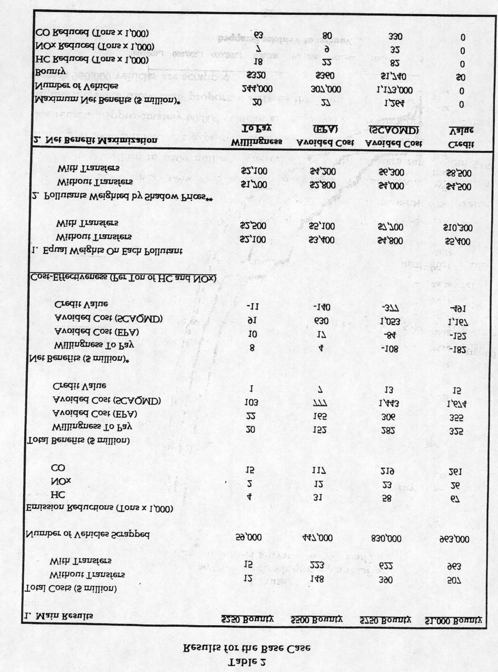
23 assumed to be in place. The impact of a more stringent, "enhanced" inspection and maintenance program will be considered in the sensitivity analysis. The Scrappage Supply Curve The scrappage supply curve for the Base Case is shown along with other scenarios in Figure 2. The curve is truncated at $2,800 for purposes of presentation. As can be seen from the figure, the, lowest priced vehicles in the fleet are valued around $140. All of the supply curves exhibit the same general shape. As can be seen from the figure, the 50/50 Case and the Base Case fall between the two extreme scenarios of all fair and all good. Base Case Results The results for the Base Case are shown in Table 2. The costs, cost-- effectiveness and benefits are calculated for four different bounties - $250, $500, $750, and $1,000. Costs increase more than proportionately as the bounty increases because of the upward sloping supply curve. Note that costs vary dramatically, depending on whether transfers are included. As can be seen from Figure 2 and Table 2, as more vehicles are scrapped, the discrepancy between the two measures of costs increases. At a bounty of $1,000, for example, the cost without transfers is about $500 million, and with transfers is about $960 million, representing a sizable difference. For bounties between $250 and $1,000, costs without transfers range from around $10 million to $500 million, whereas costs with transfers range from $15 million to $960 million. As expected, as higher bounties are offered, more vehicles are retired. Approximately 60,000 vehicles are scrapped at a bounty of $250, and this figure increases more than proportionately as the bounty is increased to $1,000, at which 960,000 vehicles are scrapped.

24

25

26 Emission reductions range from about 2,000 tons for NOx in the low bounty case to about 260,000 tons of CO for the high bounty case. In all cases, however, emission reductions are less than 10% of the total inventory. For the case of a $250 bounty, emission reductions are less than 1% of the total emissions for each pollutant. 22 For the case of $1,000 bounty, emission reductions are between 5% and 10% of the total emissions for each pollutant. Cost-effectiveness yields an opposite pattern to costs. Using both measures of cost, as the bounty increases and more vehicles are scrapped, cost-effectiveness steadily gets worse, regardless of the relative weights on HC and NOx. This is due to two factors: (1) costs are increasing, and (2) higher bounties attract newer, cleaner vehicles. Four calculations of benefits are also shown in Table 2. In all cases, the benefits using the SCAQMD avoided cost measure are the highest, simply because these numbers represent the highest marginal valuation for each ton of pollutant reduced for all three pollutants. To calculate net benefits, the costs of scrappage without transfers are subtracted from the total benefits. As shown in the table, net benefits are negative in some cases and positive in others. The table also provides some insight into the appropriate bounty for a program if the aim is to maximize net benefits. Depending on the measure of benefits selected, the appropriate bounty would vary between $0 and $1,740. For the WTP scenario, net benefits are maximized at a bounty of $320. Net benefits reach a maximum value of $20 million using WTP values, $27 million using EPA avoided 22 Estimates of the total yearly emissions of HC, NOx and CO in Los Angeles County are derived from CARE (1991b). Yearly emissions of HC, NOx and CO are estimated to be 290,000 tons, 270,000 tons and 1,100,000 tons, respectively. In this analysis, the total emissions for each pollutant are calculated for a three-year period because this is the assumed remaining lifetime of the scrapped vehicles.

27 costs, $1.3 billion using SCAQMD avoided costs and $0 using actual credit prices. The optimal number of cars scrapped varies between 0 and nearly 1.2 million. In the case where actual credit prices are used, there is no scrappage at all because the marginal benefits of reducing pollution are relatively low. The results for the Base Case and the various sensitivities are summarized in Tables 3a, 3b and 4. Table 3a summarizes program size, emission reductions and cost-effectiveness results; Table 3b highlights the costs and benefits associated with different bounties; and Table 4 presents information on net benefit maximization. 4.2 The Effect of Varying Fleet Condition The effect of varying fleet condition is shown in Figure 2 above. For a given bounty, the most vehicles are scrapped in the Fair Case because vehicles have the lowest book values there. The fewest vehicles are scrapped in the Good Case because vehicles have the highest book values there. Note the similarity between the supply curves for the Fair Case and the Base Case. This reflects the fact that a large fraction of the low-valued cars in the Base Case are presumed to be in fair condition. The results also exhibit some similarities across all four cases. For the four bounties considered here, cost-effectiveness is quite similar for the Base Case, the 50/50 Case, the Fair Case and the Good Case. For example, cost-effectiveness without transfers at a bounty of $500 ranges from a low of $3,400 per ton to a high of $4,700 per ton when HC and NOx are weighted equally. When the two pollutants are weighted by their shadow prices, these numbers fall to $2,800 and $3,900, respectively. The only case for which cost-effectiveness is not similar is the $250 bounty. For this bounty, no cars are scrapped in the Good Case because the values of all vehicles exceed $250.

28

29

30

31 The point at which net benefits are maximized is also quite similar for the four cases. The optimal bounty is about $300 using WTP numbers or avoided cost numbers from EPA. It jumps to about $1,800 using avoided costs numbers from the SCAQMD, and is $0 for the case in which credit prices are used as a benefit measure. 4.3 Sensitivities on the Replacement Vehicle The choice of a replacement vehicle is one of the key variables in assessing scrappage over which there is great uncertainty. The Base Case uses a replacement vehicle with "typical" emissions that is driven the same number of miles as the scrapped vehicle. This section considers sensitivities on both of these factors. First, vehicle miles traveled by the replacement vehicle are reduced by ten percent and increased by ten percent. Next, a new car is used as a replacement vehicle. The qualitative impacts of these changes can be predicted. First, note that they only affect the net level of emissions reduced. When vehicle miles traveled are reduced relative to the Base Case, this increases the amount of emissions reduced per scrapped vehicle and thus improves cost-effectiveness, total benefits and net benefits. On the other hand, when vehicle miles traveled by the replacement vehicle are increased, just the opposite results obtain. The same qualitative impact of a decrease in vehicle miles traveled accompanies the use of a new vehicle as the replacement vehicle - i.e., net emissions reductions increase because a new car is cleaner than a typical car. This change leads to a significant improvement in cost-effectiveness and enhanced benefits at a given bounty. Tables 3a, 3b and 4 provide information on the magnitude of these changes. First consider a 10% decline in VMT. For the lowest bounty, emission reductions

32 and benefits increase on average by 7%; however, as the bounty increases and more vehicles are scrapped, emission reductions and benefits increase by more, averaging nearly 10% at a bounty of $1,000. Cost-effectiveness also improves as the bounty increases, but by slightly less than emission reductions and benefits. Due to higher emission reductions, net benefits increase in all cases, but by varying magnitudes. For example, when SCAQMD's avoided cost numbers are used as benefits, net benefits in the 90% VMT Case increase by an average of 11% relative to the Base Case; however, when credit values are used to measure benefits, this increase is less than 1%. Next, consider the case where VMT increases by 10%. Analogous to the previous case, there is a fall in emission reductions and benefits, but in this case the reduction averages only 8%. Costeffectiveness gets worse by an average of 7%. Net benefits fall relative to the Base Case, but, as in the 90% VMT Case, the size of the decrease varies depending on how benefits are measured. Using a new vehicle as the replacement vehicle yields a substantial improvement over the Base Case. Emission reductions and benefits nearly double and cost-effectiveness improves by roughly a factor of two. The primary reason for these dramatic improvements is that a new vehicle is significantly cleaner than a typical vehicle in the fleet. Also, because benefits significantly increase while costs remain constant, net benefits climb substantially, reaching a maximum of $120 million (using the EPA avoided cost approach) compared to $27 million in the Base Case. When emission reductions increase for each vehicle, the cost per ton improves. Because the benefits per ton are constant (by assumption), it pays to scrap some additional vehicles. That is, one would expect a higher scrappage price associated with the point at which net benefits are maximized. If emission

33 reductions decrease for each vehicle, one would expect a lower scrappage price. For the cases in which vehicle miles increase and decrease by 10%, this pattern is borne out; however, the only significant change in the optimal bounty occurs when SCAQMD avoided costs are used to measure benefits, in which case the difference is as much as $160. For the case in which a new car replaces the typical car, the change in optimal bounties is more pronounced. Optimal bounties increase by more than $200 for all but the credit value case. The credit values are not sufficiently high to generate scrappage in any of these scenarios. 4.4 Sensitivities on the Target Vehicle Group Choosing a particular vehicle group for a scrappage program is also a critical design parameter in that it can affect both program size and economic performance. Programs targeted at older vehicles typically will retire fewer cars, cost less and reduce fewer emissions than will programs that offer eligibility to more vehicles. 23 However, as this analysis shows, these smaller programs are likely to be more cost-effective than larger ones, particularly because larger programs allowing more model-years have a greater chance of retiring cleaner vehicles. Sensitivity analyses are conducted on subsets of the fleet that are both smaller and larger than the subset used in the Base Case. 24 The results of these sensitivities are shown in Tables 3a, 3b and 4. In the Pre-1978 Case, the pool of eligible vehicles is smaller than it is in the Base Case, and as expected, the number of vehicles retired, total costs and emission reductions are all lower than in the Base Case. However, cost-effectiveness is lower at all bounty levels in the Pre-1978 Case, falling by as much as $600 per ton at a bounty of $1,000. Finally, net benefits are maximized in 23 Some scrappage programs place limits on the number of vehicles they will retire, in which case placing model-year-based restrictions on eligibility may or may not affect overall program size. 24 The Base Case is equivalent to what could be labeled the 'Pre-1980 Case." 21

34 the Pre-1978 Case at bounties greater than or equal to the Base Case, reflecting the fact that the marginal cost per ton reduced has decreased at a given bounty while the marginal benefit remains constant. Relative to the Pre-1978 Case, the Pre-1979 Case expands the eligible scrap fleet to include one more vehicle model-year. Making this change brings in roughly 8,000 more vehicles at a bounty of $250, but the total is still 3,000 vehicles short of the total in the Base Case. All performance measures of the scrappage program in the Pre-1979 Case (i.e. costs, benefits, costeffectiveness, etc.) fall in between those from the Base and Pre-1978 Cases. The Pre-1981 Case targets a larger subset of the fleet than the Base Case and, relative to the Base Case, attracts 1,000 more vehicles at a bounty of $250 and 114,000 more vehicles at a bounty of $1,000. Total costs, emission reductions and benefits all increase relative to the Base Case; however, net benefits in the Pre-1981 Case are generally lower, as are the optimal bounties at which they are maximized. When a pre-1982 target is considered (as well as when all vehicles in the fleet are eligible), the trends shown in the Pre-1981 Case continue. The number of vehicles, total costs and emission reductions all increase, but cost-effectiveness gets worse as more vehicles become eligible to participate in the program. This is primarily due to the scrapping of some cleaner vehicles. Total benefits increase relative to the Base Case, while net benefits decrease. Also, the optimal bounties at which net benefits are maximized decline as well. For example, while the optimal bounty using SCAQMD benefits is $1,740 in the Base Case, it is only $1,200 in the Pre1982 Case and $800 in the All Vehicles Case. A review of all five of the scenarios involving different vehicle populations suggests that the maximum net benefits do not vary much when the benefits

35 measure used is based on credit values, willingness to pay or EPA avoided cost numbers. Moreover, the optimal bounty is remarkably stable across these scenarios for each of these measures of benefits. For example, the optimal bounty is $0 when credit values are used to measure benefits and between $300 and $400 when EPA and willingness to pay numbers are used. In contrast, the optimal bounty exhibits greater variation across the vehicle scenarios when the SCAQMD numbers are used. Here, the bounty decreases in order to reduce the number of relatively clean vehicles selected in a scrappage program. This explains why the optimal bounty in the All Vehicles Case is about $900 lower than in the Base Case. 4.5 Discounting Emission Reductions This analysis discounts emission reductions from scrapping each vehicle back to the present in order to make these reductions comparable to costs.25 A discount rate of 5% is used in the Base Case. Changing the discount rate from 5% to 10% only affects the emission reductions beyond the first year. Relative to the Base Case, the reduction in the present value of emission reductions leads to a noticeable decline in cost-effectiveness, total and net benefits. While the optimal bounties generally remain unchanged, maximum net benefits when the discount rate is 10% fall below those in the Base Case. 4.6 The Effect of Enhanced Inspection and Maintenance The interaction between programs is a critical variable in the design of judicious policies for regulating the automobile (Lave, 1981). Changes in the inspection and maintenance (I&M) programs throughout the U.S. could have a dramatic impact on the viability of scrappage programs. The Base Case assumes that 25 A more complete model would include the impact of the discount rate on differences in operating and maintenance costs over time.

36 the 1990 California I&M program is in place. The Clean Air Act Amendments of 1990 call for a more rigorous I&M program. Over the past few years EPA has been developing an all-new Enhanced I&M program, which is scheduled for introduction in This analysis examines the impacts of Enhanced I&M on reducing vehicle emissions, as well as the additional costs of such a program. EPA estimates that Enhanced I&M will have a significant impact on vehicle emissions.26 For passenger cars, a reduction of nearly 27% is expected for total exhaust and evaporative hydrocarbons. Considering exhaust emissions only, reductions of 8%, 10% and 1% are expected for HC, CO and NOx, respectively. For light-duty trucks, even more emission reductions are anticipated. Total exhaust and evaporative HC emissions are expected to fall by roughly 34%, as are exhaust HC emissions alone. Also, EPA estimates reductions in tailpipe CO and NOx to be around 39% and 9%, respectively. Lower emissions resulting from Enhanced I&M means that the emission reductions from scrappage will most likely fall. To model the cost impact that may result from Enhanced I&M, this analysis focuses on the incremental costs for each vehicle. Calculating costs in this manner involves several steps. First, the additional costs for an inspection must be determined, and, based on calculations in EPA (1992b), a figure of approximately $40 is used here.27 The second step in calculating the incremental costs per vehicle is to consider repair costs. A wide range of costs has been estimated for what it would take to fix the vehicular malfunctions that are likely to be uncovered using the Enhanced I&M procedure. Based on estimates by EPA (1992b) and Anderson and 26 To determine the percent reductions in emissions, this analysis calculates the difference between EPA's emission factors in a Basic I&M scenario and in the proposed Enhanced I&M scenario. See Appendix I in EPA (1992b). 27 This $40 figure is the incremental inspection cost calculated by EPA for a decentralized Enhanced I&M system and, as the current I&M network in California is decentralized, is appropriate for this analysis.

37 Lareau (1992), this analysis uses a figure of $125 as the average repair cost per vehicle under Enhanced I&M. Because not all vehicles will incur this repair cost, some estimate of the probability of failing an Enhanced I&M test is needed. Because reliable data on failure rates for Enhanced I&M do not exist at this time, this analysis uses estimates of failure rates for California's current I&M program (Sierra Research, 1993). 28 Combining inspection costs with, failure probabilities and repair costs permits the calculation of the cost per vehicle for Enhanced I&M over the remaining life of each vehicle. 29 In order to determine the net change in costs due to Enhanced I&M, the Enhanced I&M costs for the replacement vehicle must be subtracted from the costs for the original vehicle to produce a net Enhanced I&M cost for each vehicle. The incremental cost for the replacement vehicle is found using the additional $40 inspection cost and $125 repair cost along with the average failure probability over the entire fleet. The final step in incorporating these incremental costs into the scrappage decision is to subtract the net Enhanced I&M cost for each vehicle from its book value to yield its "effective" book value. The effect of this subtraction can be to either decrease or increase the effective book value of a vehicle. For older vehicles in the fleet whose expected Enhanced I&M costs are likely to exceed those of the average replacement vehicle, the effective book value is necessarily less than the original book value. Such is the case for pre-1980 vehicles, and as shown in 28 Small sample data from EPA (1992b) indicate that failure rates under Enhanced I&M are likely to be much higher than they currently are for existing I&M programs. However, it is quite possible that the improved testing and repair under Enhanced I&M will lead to a decline in these failure rates over time (Austin, 1993). 29 The actual calculation of these costs is as follows; Cost Per Vehicle = Probability of Failure * (Inspection Cost + Average Repair Cost) + (1 - Probability of Failure) * Inspection Cost. In year 2, the failure probability for a model-year T vehicle is assumed to be equivalent to the year 1 failure probability of a model-year (T-1) vehicle.

38 Figure 3, this leads to slightly more scrappage at a given bounty. Just the opposite is true for newer vehicles. Incorporating an Enhanced I&M program into the Base Case has several effects on the performance of the scrappage program. As stated above, the number of vehicles increases when Enhanced I&M is phased in, although at higher bounties fewer vehicles are added. For example, at a $250 bounty, Enhanced I&M leads to the scrappage of roughly 140,000 more vehicles than in the Base Case; however, at a $1,000 bounty, only 7,000 more vehicles are scrapped. This can also be seen graphically in Figure 3. Emission reductions, total and net benefits under Enhanced I&M are much higher than in the Base Case at a bounty of $250. This increase is a direct result of the increase in the number of vehicles retired when Enhanced I&M is in place. At bounties of $500 and higher, however, they are lower than in the Base Case, due to the fact that the I&M program is expected to make the fleet much cleaner overall. The cleaner fleet in the Enhanced I&M Case also leads to a worse cost-effectiveness in the scrappage program, regardless of the bounty. Finally, maximum net benefits in the Enhanced I&M Case fall short of those in the Base Case, as do the optimal scrappage bounties. 4.7 Comparing Scrappage with a Vehicle Emissions Trading Program that Allows Scrappage The primary difference between a scrappage program and a vehicle emissions trading (VET) program is that the scrappage program retires vehicles that may not be cost-effective to retire at specific credit prices under a VET program. Some of these vehicles may result in net increases in emissions, while others may be scrapped even though the value of their net emission reductions falls short of the value that would be required if a VET program were in place. To capture the difference in the types of vehicles scrapped in the two programs, a VET program with a given cost,

39

40 measured in terms of the value of vehicles scrapped, is compared to a scrappage program with the same cost. The first step in the analysis is to identify those vehicles that would be scrapped under a VET program at a specified set of credit prices. The next step is to calculate the cost of scrapping those vehicles. The final step is to examine the characteristics of a scrappage program in which the costs are just equal to those incurred under the VET program. Two sets of credit prices are considered for a VET program: one given by the EPA avoided cost numbers -- $3,050/ton of HC, $2,750/ton of NOx and $300/ton of CO; and a second given by the SCAQMD avoided cost prices of $8,500/ton of HC, $30,000/ton of NOx and $1,200/ton of CO. The results of this analysis are shown in Table 5. Approximately 200,000 more vehicles are scrapped under the scrappage scenario because this scenario selects some low-value cars that are not selected in the VET scenario. When benefits are evaluated at the specified credit prices, net benefits are lower under scrappage for the same reason.30 Emission reductions also decline or stay roughly the same under scrappage for HC and NOx, although CO reductions actually increase under scrappage. The principal quantitative result that emerges from the analysis is that scrappage is quite similar to a VET program with credit prices that equal EPA avoided costs. Indeed, there is only a $400,000 difference in net benefits of the two programs. When SCAQMD avoided costs are used as credit prices, the differences between scrappage and a VET program become slightly more pronounced, with net benefits under a VET program exceeding those from scrappage by over $2 million. It is important to note that, because scrappage allows 30 If benefits were measured at something other than their credit price, this result need not obtain. See, e.g., Oates, Portney and McGartland (1989).

41

42 the retirement of more vehicles than a VET program does, making more vehicles eligible candidates for scrappage would most likely increase the differences shown in this analysis, primarily because the chances of a scrappage program retiring some clean vehicles would be higher Capturing Dynamic Aspects of a Scrappage Program A key question related to a scrappage program is how it would perform over time. Under the assumptions of the preceding analysis, the cost-effectiveness of a scrappage program is likely to worsen over time, as clean cars with lower deterioration rates replace vehicles that pollute more. To capture this effect, a simulation is run which fixes the scrappage bounty in the first year, updates the fleet, and then offers the same scrappage bounty or a higher one in the following year. The fleet is updated in a stylized manner. Only vehicles not scrapped in the first year are presumed to be candidates for scrappage in the second year. Book values in the second year are assumed to decline by 10% for each vehicle. Emission reductions are adjusted to reflect that each remaining car is now one year older. Two scenarios are considered: one in which the initial bounty is $500 in year 1 and subsequent bounties are $500, $750 and $1,000; and a second in which the initial bounty is $700 in year 1 and subsequent bounties are $750 and $1,000. These bounties were selected because they are in the range of bounties that are considered for actual applications. 31 This analysis ignored the possible transactions costs associated with scrappage or a vehicle emissions trading program (Stavins, 1993). If, for example, it is more costly for vehicle owners to participate in one program as opposed to the other, this could affect the outcome. Obviously, different administrative costs across programs could also affect the welfare analysis.

43 The dynamic effects of scrappage are shown in Table 6 for the two scenarios. The first and the second scenario are similar. For the first scenario of la $500 bounty in the first and the second year, emissions reductions decline substantially because the number of cars scrapped declines dramatically from 447,000 to 128,000. As the bounty increases to $750 and $1,000 in the second year, emission reductions increase, simply because many more vehicles are scrapped. Scrapping all of these vehicles, however, increases costs significantly, and this has an: adverse impact on cost-effectiveness. Cost-effectiveness is consistently better in the first year than in the second year because most of the dirtiest cars are removed in the first year. Also, these dirty vehicles are inexpensive (i.e. $500 or less), so costs are relatively low in the first year. Because costs increase and cost-effectiveness decreases, net benefits can be expected to decrease as well. As can be seen from the first simulation, net benefits in the first year are significantly higher than they are in the second year. This analysis shows that the benefits from scrappage are likely to decline significantly over time. Thus, scrappage is best viewed as a short-term strategy for cost-effectively reducing a small part of the air pollution problem. 4.9 Comparing Results With Other Studies A comparison of the results developed here with those of OTA (1992) and CARE (1993a) is shown in Table 7., The cost-effectiveness numbers used for comparison are those with transfers because the other studies do not separate transfers from direct costs to the individual. The cases used for comparison are those most closely resembling the scenarios used in other studies. The general magnitude of the results is quite similar, suggesting that if these other studies estimated cost-effectiveness without transfers using the method employed here, the

44