wb Thermodynamics 2 Lecture 10 Energy Conversion Systems

Transcription

1 wb Thermodynamics 2 Lecture 10 Energy Conversion Systems Piero Colonna, Lecturer Prepared with the help of Teus van der Stelt Delft University of Technology Challenge the future

2 Content Lecture 10 - overview Steam power plant (Rankine cycle) Superheating and reheating: thermodynamics Cycle with regenerator, supercritical cycle Organic Rankine Cycle Refrigeration: compression cycle (inverse Rankine) Brayton cycle (Gas Turbines) Ideal vs real Brayton air cycle Regeneration Closed Brayton Cycle 2

3 Superheating and reheating The steam turbine: high expansion ratio ( P =1884) and problem of condensation Our example: quality q 4 =0.81. Max for current turbines q 4 =0.9 From Carnot: increase of P is beneficial: thermal energy introduced at higher T Reheating 3

4 Supercritical cycle Efficiency: cycle Limit: materials T T max min Best steam power plants: (ultra) supercritical 300 bar and 630 C, cycle = 48 % 4

5 Regeneration (1) Need for dearation Difference from Carnot Cycle Large inefficiency liquid preheating with steam spilled from the turbine 5

6 Regeneration (2) Positive and negative effect Ideal: continuous regeneration = Carnot ( Arab phoenix ) Common to all modern ECS and processes (heat integration) 6

7 Example: evaluation of regeneration Data as in the superheated cycle Steam extraction at 7 bar. It provides heating from 2 to 3 5 Need to calculate state 3, 4, and 6 5 sat T 4,is 4 P 2 3,4 6 3 s P 1 4 is 7 7

8 State 3 (dearator) T 4,is 4 P s P 1 5 sat 3,4 6 4 is 7

9 T 4,is 4 P s P 1 5 sat 3,4 6 4 is 7

10 Organic Rankine Cycle turbogenerator Small capacity: from few kw up to 1-2 MW e (optimal turbine) Renewable energy! Good for low-temperature heat sources (geothermal) Dry expansion Analysis: the same as steam cycle, but different fluid 10

11 Refrigeration Vapor compression cycle Objective: cooling, thermal energy transfer (food, home,..) Inverse Rankine cycle (same cycle shape in the T-s and P-h diagrams) Thermal power transfer is obtained by means of mechanical power (compression) Working fluid: refrigerant to match environment conditions 11

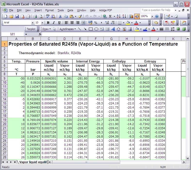
12 Vapor comp. cycle analysis: Input data INPUT DATA Working fluid: R245fa Evaporation temperature: T = K Condensation temperature T = K Compressor: is, compr =

13

14 Refrigeration cycle: Anaysis (1)

15 Refrigeration cycle: Anaysis (2)

16 Calculation of the COP

17 Q IN Brayton cycle Q OUT Advantage of a gas cycle (simple, light) Why gas turbine came after steam engines Working fluid: air (ideal gas) Q IN Operating principle Processes Q OUT 17

18 Brayton cycle calculation: Input data INPUT DATA: operating parameters State 1, K (20 C), bar (atmospheric pressure) State 2, 0.4 MPa (4 bar) State 3, K (525 C), 0.4 MPa (4 bar) State 4, bar INPUT DATA: components efficiencies Compressor: is, comp =0.65 Turbine: is, turb =0.85 Same as in the Rankine Cycle example 18

19 Assumptions Kinetic and potential energies negligible at states 1, 2, 3, and 4 Compressor and turbine adiabatic No pressure drop in the heater The system is at steady state Equilibrium states at 1, 2, 3, and 4 Air can be modeled as a polytropic ideal gas ( = 1.4 C p = const = 1.04 kj/kg K) or as an ideal gas with C p = C p (T) (FluidProp/GasMix) 19

20 Compressor work (state 1&2) 20

21 Air Heating (state 3) 21

22 Turbine work (state 4) 22

23 Net power output and efficiency Comparison with Superheated Rankine cycle for similar compression and expansion efficiencies, but higher TIT. I,Rankine II,Rankine

24 Efficiency of the ideal Brayton cycle Pv RT, c const., isentropic compression/expansion divide and multiply by T 1 w q c T T T T 1 T q q c T T T T 1 T net out P in heater T4 T3 T1 1. T T T T T T 3 P 2 T P P 3 2 divide and multiply by T2 P2 P P P P Depends only on and = 1.6 = 1.4 =

25 Ideal gas cycle W net max for T 4 = T T 3 = T w net (w net,max ) lim w net [kj/kg]

26 Comparison real vs ideal cycle The most relevant losses are in the compressor and turbine: limitation of ideal-gas analysis ( too high is a problem) Limit on TIT (blade cooling) Fuel issue 26

27 Gas Turbine Advantages: High temperature & low pressure -> high power/weight No blade erosion with high-quality fuel Fast load-change Applications: Aircraft propulsion (ships, trains) Combined Cycle, Peak-shaving Cars (for hybrid engines in the future?) 27

28 Gas turbine cycle: parameters Ideal ( max, TIT) TIT = 1400 C C TIT = 800 C 900 C 1000 C

29 Regeneration Reduction of thermal losses Note: T 4 often in excess of 450 C For given TIT, maximum efficiency at modest (increase T 4 T 2 ) Recuperator: technological problem 29

30 Closed Brayton cycle gas turbine 30

31

32 Final remarks Importance of assumptions Always mass and energy balances Thermodynamic cycles: comparison with Carnot cycle Courses on gas turbines of the Master in Sustainable Energy Technology: WB4420 Gas Turbines and WB4421 Gas Turbines Simulation/Application 32