Cornelia Hesse, Valentina Krysanova and Fred Hattermann Potsdam Institute for Climate Impact Research

Transcription

1 Identification of point and diffuse sources and role of retention processes in large river basins: comparison of three approaches Cornelia Hesse, Valentina Krysanova and Fred Hattermann Potsdam Institute for Climate Impact Research

2 Outline 1. Case study basin: Saale 2. Model SWIM 3. Three approaches for nutrient retention in large basins 4. Step 1: retention in the landscape - three pathways 5. Step 2: retention in the landscape - differentiation of retention coefficients for three pathways 6. Conclusions and outlook

3 Diversity of landscapes in the Elbe basin

4 Case study basin: Saale Second largest tributary of the Elbe Length 413 km Drainage basin ~ km²

5 Case study basin: Saale

6 SWIM (Soil and Water Integrated Model) Climate: Global radiation, temperature, precipitation Hydrological cycle Nitrogen cycle Soil profile A B C Vegetation/ Crop growth LAI Bio mass N-NO 3 N o-ac N o-st N res Phosphorus cycle SWIM was developed in PIK (Potsdam) based on SWAT-93 and MATSALU for climate and land use change impact studies Upper ground water Lower ground water Roots Land use pattern P lab P m-ac P m-st & land management P org P res

7 Spatial disaggregation Subbasins Land use Soils +... Hydrotope Hydrotops are sets of units in subbasins with uniform land use and soils

8 From the hydrotope to the basin level Climate Hydrological cycle A B C Vegetation LAI Roots Bio mass N cycle N-NO 3 N o-ac N o-st N res P cycle P lab P m-ac P m-st P org P res Land use pattern

9 Nutrient retention in watersheds: 3 approaches Three approaches: 1) retention in a landscape is described separately for surface, subsurface and groundwater flows by a linear differential equation (Hattermann et al., 2005) as a function of mean residence time T and decomposition rate λ, with constant T sur, T sub, T gw and λ sur, λ sub, λ gw for the basin; 2) the same as in the first approach, but differentiating T sur, T sub, T gw and λ sur, λ sub, λ gw for hydrotopes depending on soil properties and g-w conditions; & 3) coupling SWIM with the model WASP to additionally describe retention processes in the river network in combination with approaches 1 or 2.

10 r c u Dg σ + c c + λc + t R R R c = concentration n = eff. porosity m = aquifer thickness λ = turnover coeff R = faktor of retardation Approach 1: nutrient retention q mn f R ( c c ) = 0 Simplifications: Full mixture during the transport process Residence time is normally distributed Linear degradation dct dt = C t, in Ct, out λ C t C t = KC t, out 1 (1/ K+ λ) t (1/ K+ λ) t Ct, out = Ct, in (1 e ) + Ct 1, oute 1+ Kλ in Classical approach: the convection-dispersion equation But: -it is nonlinear and has to be solved numerically - high data demand K = mean residence time, λ = decomposition rate, C = concentration

11 Approach 1: The mean residence time K = n i i= 1 vs ( zi ) dz The mean residence time K = f (flow path, permeability, porosity, gradient in groundwater table) for subsurface flow K = f (flow path, permeability, porosity, and gradient in topography and Manning s roughness) for surface flow. L = n i= 1 dz i The distance L to the river is calculated following the gradient in groundwater table to the river. k * J ( z) v s ( z) = S K can be estimated using the seepage velocity v s (m d -1 ), where k is hydraulic conductivity of the spatial unit z, J is dimensionless hydraulic gradient, and S is the specific yield (average ~40 years, up to > 1000 years).

12 Approach 1: The decomposition rate The decomposition rate λ is a function of redox potential and carbon concentration of the catchment sediments. Initial values can be established using data from Wendland et al. (1993): a half-life time of nitrate N between 1 and 3 years, which corresponds to λ values between d -1 and d -1.

13 Validation using first approach: water discharge W ater discharge, Calbe-G rizehne, E = 0.81 m³/s Q obs Q sim

14 Validation using first approach: N-NO 3 load E = meas [kg/d] sim [kg/d] E = meas [kg/d] sim [kg/d]

15 Approach 2: differentiated retention coefficients Nutrient retention in a landscape is described separately for surface, subsurface and groundwater flows as a function of mean residence time T and decomposition rate λ, and T sur, T sub, T gw, λ sur, λ sub, λ gw are differentiated depending on soil properties and g-w conditions.

16 Estimation of Denitrification conditions in soils of Central Europe Soil water nutrients temperature PH TOTAL + good conditions for D: gley, pseudogley, loess, marsch, moor, tschernosem O neutral conditions for D: brown soils, parabrown soils, rendzina, pararendzina poor conditions for D: podsol, podsol-brown soils, syrosem Wendland et al. Atlas zum Nitratstrom in der Bundesrepublik Deutschland

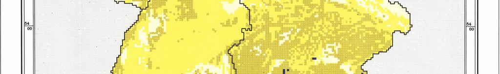
17 Denitrification conditions in soils, Germany + loess soil O brown soils podsol Wendland et al. Atlas zum Nitratstrom in der Bundesrepublik Deutschland

18 Aggregation of soil types for the II approach 45 SWIM soil types 14 denitrification soil types 3 denitrification categories poor conditions neutral conditions good conditions

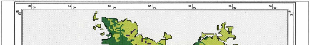
19 Denitrification conditions in groundwater, Germany unlimited limited insignificant Wendland et al. Atlas zum Nitratstrom in der BUndesrepublik Deutschland

20 Conclusions and outlook Water quality modelling in large river basins should include consideration of retention processes on the way to river network. The I hypothesis to be proved: in large river basins the residence time and decomposition rate should be differentiated based on soil properties and groundwater conditions. The II hypothesis to be proved: in large river basins description of nutrient retention processes in river (e.g. coupling SWIM with WASP or QUAL2E) is needed to better represent water quality.