5. Using SLAMM. Introduction... 25

Transcription

1 5. Using SLAMM Introduction... 2 Hardware Requirements and Recommendations... 3 Description of the Files Associated WinSLAMM... 4 WinSLAMM.EXE... 4 MPARAXX.EXE... 4 MSCALCXX.EXE... 4 Creating or Editing a SLAMM Data File... 4 Introduction... 4 Starting the Program... 5 Main Data Entry Form... 6 Current File Data Button... 8 Data Entry Pollutant Analysis Selection Information Saving the Data File Creating WinSLAMM Output Parameter Module Description Introduction Rain Input Subprogram Description of Selected Rainfiles Included With The Program Runoff Coefficient Subprogram Critical Particle Size Subprogram Description of Selected Critical Particle Size Files Included With The Program Particulate Solids Concentration Module Particulate Residue Reduction Subprogram Pollutant Probability Distribution Subprogram Example Input and Output Files Typical Land Use Descriptions General Land Use Descriptions Land Development Characteristics Site Surveys Area Measurements from Aerial Photographs Example Land Use Evaluations for Los Angeles County, California Little Shades Creek (Rocky Ridge Corridor) Preliminary SLAMM Analyses WinSLAMM Calibration Procedures Runoff Coefficients Initial Data Sources Calibration Steps Particulate Solids Concentrations Initial Data Sources Calibration Steps Pollutant Concentrations Appendix 5-A: Shades Creek Land Use Descriptions Residential Areas Low Density (LDRCB.DAT and LDRSB.DAT)

2 Medium Density, pre 1960 (MR6CB.DAT and MR6SB.DAT) Medium Density, (MR68CB.DAT and MR68SB.DAT) Medium Density, since 1980 (MR8CB.DAT and MR8SB.DAT) High Density (HDRCB.DAT and HDRSB.DAT) Multi-Family (Duplexes) (MFRCB.DAT and MFRSB.DAT) Apartments (APTCB.DAT and APTSB.DAT) Commercial Areas Strip Development (STRCB.DAT and STRSB.DAT) Shopping Centers (SHPCB.DAT and SHPSB.DAT) Office Parks (OFFCB.DAT and OFFSB.DAT) Institutional Areas Schools (SCHCB.DAT and SCHSB.DAT) Industrial Areas Light Industry (Warehousing) (LIDCB.DAT and LIDSB.DAT) Open Space Golf Courses (GLFCB.DAT and GLFSB.DAT) Cemeteries (CEMCB.DAT and CEMSB.DAT) Parks (PRKCB.DAT and PRKSB.DAT) Undeveloped (UNVCB.DAT and UNVSB.DAT) Freeway Areas Freeways (FRYCB.DAT and FRYSB.DAT) Appendix 5-B: WinSLAMM Algorithm Documentation Introduction Data Entry Control Devices Data File Format Calculation/Output Module Calculations Calculation/Output Module Overview Calculation/Output Module - Output Appendix 5-C. Bham76.ran File Printout Appendix 5-D. Runoff.rsv File Printout Appendix 5-E. Delivery.prr File Printout Appendix 5-F. Bham.psc File Printout Appendix 5-G. Bham.ppd File Printout Appendix 5-H. Medium.cpz File Printout Introduction This section is a detailed discussion of the calculation procedures developed for the original DOS based version of SLAMM and now found in the Windows version, WinSLAMM. Over the past few years, the program was completely re-written in Visual Basic, version 5, to be completely Windows-based. The current version is numbered 8. Version 6 added Monte Carlo components to the model, developed with funding from Region 5 of EPA. Version 7 was a hybrid version, using many of the older DOS calculation modules, but with the initial windows user interface modules. It also included numerous additional changes. This version 8 is the first complete Windows-based version (including the basic data input, calculation, and output modules found in the DOS version) and closely resembles version 7 in content and capabilities, with a few additional changes. We are planning a new version 9 soon to incorporate many new features from our recent stormwater research conducted over the past several years. The main changes made to the program since the original user guide and algorithm documentation was prepared include the following: Practically all of the variable names given in this section and the use of goto statements have been changed to reflect current programming practice. The HELP files in the model provide accurate guidance for the model in its present form. Most of the parameter file maintenance programs are still DOS-based, but 5-2

3 have been modified. SLAMM can now easily evaluate large rain files - analyses containing more than 4 decades of data and many thousands of individual rain events have been successfully conducted. Monte Carlo stochastic components have been added to the pollutant calculations to provide better representations of the random nature of stormwater pollutants. The batch processor program, originally developed for the DOS program, was modified for use with the Windows-based program. It now works with users interfacing WinSLAMM with GIS programs. Selected processes have been corrected or changed to reflect bug fixes or process modifications. These changes include adding additional controls and flexibility for the analyses of detention ponds, more accurate descriptions of catchbasins in an area, and modifying the pollutant listing. An interface program for the use of WinSLAMM as a replacement for the RUNOFF block in SWMM was developed as the main activity of the EPA-sponsored activity reported in this report. WinSLAMM (the Windows version of the Source Loading And Management Model) is an urban rainfall runoff water quality model. It calculates runoff volumes and urban pollutant loadings from individual rain events. It also allows the user to reduce pollutant loadings from a source area such as a roof or street area by using control measures such as detention ponds or infiltration devices. The model is in many ways a very large pollutant mass and flow accounting program. Runoff volumes are calculated by multiplying the rain depth by varying runoff coefficients. The resulting source area runoff volumes are then multiplied by particulate residue concentrations to get particulate residue loadings for each source area for the rain. The runoff coefficient is a function of rain depth, land use (eg, a residential land use), and source area. The particulate residue concentrations are a function of runoff depth, land use and source area. Other particulate pollutants are then related to the particulate residue values, while filterable pollutants are related to the runoff volumes. Much of the program is devoted to identifying the appropriate runoff and particulate residue concentration values for a given rain depth, land use, and source area. The process is complicated by the large number of source areas within each land use and by the large number of variable combinations needed for a specific source area. Hardware Requirements and Recommendations WinSLAMM runs on personal computers under Windows 95, Windows 98, or Windows NT. The following computer features are required: Memory Requirements: The model uses many dynamic, or variable-size, arrays. If a computer runs out of memory, either reduce the number of WinSLAMM source areas and rainfall events, or close other programs that are running on your computer. A typical Pentium computer can analyze a typical situation in a few seconds to a few minutes, even for a complete set of many rain years. The addition of detention ponds or a long list of pollutants in an analysis will significantly increase the computer computational time. Disk Storage: The model creates and erases many temporary files while running. It requires only a few mb of storage on the hard drive, depending on the size of the rain files, etc. Printer: The output may be sent to a printer or saved as a file. However, output can be many columns wide, and so users may need a printer operating in landscaped mode with a small sized font to print the output. The output can also be quite extensive, so we recommend that all output be saved to a file where it can be formatted as needed. 5-3

4 Description of the Files Associated WinSLAMM WinSLAMM.EXE This Windows version SLAMM combines the DOS Input, Calculation, and Output modules of the DOS version of SLAMM. The program generates a site description file needed to run WinSLAMM, which has the extension.dat (referred to as data.dat). Besides the basic site development data requested, alternative runoff controls are also described using this program. The program must be installed using the appropriated installation files. Place the first disk in the installation drive (or the CD if you have the CD version of the installation program) and run setup from the run command or use the install new software option in the control panel, then follow the on-screen directions. The files needed to run SLAMM include: A mandatory rain.ran file to describe the rain series. A mandatory runoff.rsv file containing the runoff coefficients for each surface type to generate surface runoff volume quantities. A mandatory particulate.psc file describing the particulate residue (suspended solids) concentrations for each source area (except for roads) and land use, for several rain categories. A mandatory delivery.prr file to account for deposition of particulate pollutants in the storm drainage system, before the outfall, or before outfall controls. The DELIVERY.PRR file is calibrated for swales, curb and gutters, undeveloped roadsides, or combinations of drainage conditions. An optional pollutant.ppd file to describe the particulate pollutant strengths related to particulate residue and to describe the filterable pollutant concentrations for each source area for each land use. This file is not needed if only runoff volume and particulate residue calculations are desired. This file also contains the coefficient of variation (COV) values for each pollutant for Monte Carlo simulation in WinSLAMM. An optional size.cpz files for wet detention pond analyses to describe the runoff particulate size distributions. If no wet detention ponds are included in a WinSLAMM model, these files are not needed. MPARAXX.EXE MPARAXX is the utility program that produces, edits, and displays the above files needed by WinSLAMM. This is a DOS-based program and can be executed from the DOS prompt in the DOS shell within Windows. The example parameter files included on the disk can be printed to a file using MPARAXX.EXE and then read using any ASCII text editor. MSCALCXX.EXE MSCALCXX was the prior DOS version of the main SLAMM calculation program. It may be executed from the DOS prompt in the DOS shell within Windows. This program only asks for the data.dat file name, previously prepared using SINPXX.EXE. It automatically links with the output program. SLAMM directs all of its output to a disk file. This file can be viewed and printed using most text editors or word processors. The output format generally requires a printer in landscape mode using a small font. The Windows version executes the calculation module by using the drop-down Run menu. Creating or Editing a SLAMM Data File Introduction The information necessary to perform a WinSLAMM model run is stored in a WinSLAMM data file and its associated parameter files. This information includes a description of land uses and source areas, the time period and corresponding rainfall events, the pollutant control devices applied to the site, and the pollutants to be analyzed. 5-4

5 This section discusses how to create or edit a WinSLAMM data file that stores this information. The HELP files with version 8 of WinSLAMM offer additional direction for the current version of WinSLAMM. Table 5-1, lists the series of steps necessary to create a SLAMM data file. Table 5-1. Steps For Creating A New SLAMM Data File 1. Start the Program 2. Enter Site, Drainage, and File Information 3. Enter Data A. Land use area and source controls information B. Catchbasin and drainage control information C. Outfall control information 4. Enter Pollutant Analysis Selection Information 5. Save the Data File Starting the Program To run the program, double-click the WinSLAMM program icon or double-click WinSLAMM.EXE in Win95/98/NT Explorer. Select Open Existing File to open a file that has previously been created, select Create New File to create a new.dat file using the new file data entry sequence editor, or select Enter Main Screen to enter the data editor. Press Exit to exit the program. The opening screen for WinSLAMM is shown below. 5-5

6 Main Data Entry Form The main data entry form, which is illustrated below, allows you to enter the data needed to create a SLAMM data file. The main data entry form includes the following items: Menu items on the Main Menu bar A series of labels that identify the data file name, the current land use and source area, and the areas that have been entered for each land use A Current File Data button, described in more detail below A Current File Status button that determines if the minimum data needs of a WinSLAMM model run are met An Exit Program button A grid that lists the source areas for each land use and indicates whether source area parameters and control devices have been entered for each source area. Selecting a land use from the Land Use menu item accesses the grid for that land use. The main menu is shown below, including a view of the land use screen: 5-6

7 5-7

8 Current File Data Button The Current File Data button allows the user to enter data critical to the operation of the model. This includes parameter file names and locations, Monte Carlo seed information, model run start and finish dates, and drainage information. A list of the items in the form is described below, followed by an illustration of the form. 1. SLAMM Data File Name. File names should subscribe to all the Windows file naming conventions. Do not use any extensions; the program will add them. 2. Site description for the file. The description may be up to 230 characters long. 3. Starting date of the study period. This date must be after 1952 and should correspond to the dates of the rain events in the rain file used in this SLAMM file. The format of the dates must be MM/DD/YY or MM.DD.YY. 4. Ending date of the study period. This date must be after the starting date, and have the same format as the starting date. 5. Seed. The seed is used for Monte Carlo simulations of pollutant strength. The seed must be an integer greater than zero. Enter zero (0) for a randomly generated seed based upon the clock time a model run begins. A negative seed value will force the model to use zeros for any COV values in the pollutant probability distribution file. This has the effect of turning off the Monte Carlo pollutant loading simulation, so the model instead calculates pollutant loadings based upon the average pollutant value. 6. Rain file name. Enter the name of the rain file used in the model run. Do not include the extension. 5-8

9 7. Pollutant probability distribution file name. Enter the name of the pollutant probability distribution file you want to use for the model run. Do not include the extension. 8. Runoff coefficient file name. Enter the name of the runoff coefficient file used in the model run. Do not include the extension. 9. Particulate solids concentration file name. Enter the name of the particulate solids concentration file used in the model run. Do not include the extension. 10. Particulate residue delivery file name. Enter the name of the particulate residue delivery file used in the model run. Do not include the extension. 11. Drainage system data. Enter the fraction of the total area controlled by each drainage system type. The sum of the fractions of each of the drainage types must equal 1. The five drainage types are listed below: 1. Grass Swales. Enter additional information to characterize grass swales after entering the drainage type area fractions. This information is described in the outfall control section. 2. Undeveloped roadside. This category is used to represent haphazard drainage along a road. 3. Curb and Gutters, valleys, or sealed swales in poor condition (or very flat). This category may also be used if runoff is channeled along the edge of streets without curb and gutter. 4. Curb and Gutters, valleys, or sealed swales in fair condition. 5. Curb and Gutters, ` valleys, or sealed swales in good condition (or very steep). The printing options are included under the drop-down tab file-output options. Table 5-2 lists the main options available. There are also several one-line per event options that summarize long SLAMM runs well, especially when 5-9

10 exporting the data into spreadsheet programs for further analyses, or when using the SLAMM-SWMM interface program. Table 5-2. Printing Options 1. Print source areas by land use & outfall for each rain - complete printout. 2. Print source area totals and outfall summaries. 3. Print outfall data only for each rain. 4. Default option - Print outfall summaries only. Data Entry This section reviews the steps necessary to enter WinSLAMM land use and drainage system information into a file. The first sub-section reviews the land use area information, the second sub-section reviews the catchbasin and drainage control information, and the final sub-section reviews the outfall control information. Land Use and Source Area Information Characterize the six land uses by defining source areas. Enter source areas for each land use by selecting, from the main menu, File/{Land Use}. A data entry spreadsheet, shown below, for the land use will appear on the Main Data Entry form. This spreadsheet lists all the available source areas for the land use, the area of the source area, the available controls, and the source area parameters. To enter an area, double-click on the area column box in the row of the desired land use. You will be prompted to enter the area of the source area as well as the required source area parameter information. To enter a control for the source area, double-click on the desired control box in the row of the selected source area. Land use areas 1 to 5 each have 30 source areas, while land use 6 (Freeways) has 10 source areas, as shown below. 5-10

11 Table 5-3 is a list of the mian source areas WinSLAMM uses. In most cases, more than source area in each category is available for each land use. If a control option has been activated, the code letter for that control option will appear in the column. For example, in the data grid above, street sweeping has been activated, as indicated by the three S s in the S column. The control options available for each source area are illustrated in Figure 5-1. The information needed for each control option and the procedure to enter this information in a WinSLAMM data file is listed at the end of this section. Table 5-3. SLAMM Source Areas Roofs Sidewalks/Walks Other Impervious Areas Paved Parking/Storage Streets/Alleys Freeway Lanes/Shoulders Unpaved Parking/Storage Undeveloped Areas Large Turf Areas Playgrounds Small Landscaped Areas Large Landscaped Areas Driveways Other Pervious Areas Each source area listed in Table 5-3 has specific data requirements that depend upon the characteristics of the source area and upon the source area s land use. These requirements are listed in Table 5-4 and 5-5, which are coding forms that list the land use and control practice information requirements. These sheets should be filled out before the data file is created. 5-11

12 Streets and alleys in land uses 1 through 5 require somewhat different characteristic information than freeway (Land Use 6), paved lane, and shoulder areas. To enter a user defined street dirt accumulation equation for a street area in land uses 1 through 5, the equation must be in the form of a quadratic equation, Ax 2 + Bx + C, where A is greater than 0, B is greater than 0, and C is less than or equal to 0. Isolated areas, or disconnected areas, are areas within a land use that do not contribute runoff to the land use outfall. Isolated areas could be constructed, e.g. swimming pools, or natural land features such as kettle ponds. Source controls are not applicable to isolated areas. The source areas in the Freeway land use include Paved Land and Shoulder Areas, Large Turf Areas, an Undeveloped Area, an Other Pervious Area, an Other Directly Connected Impervious Area, and an Other Partially Connected Impervious Area. A paved lane and shoulder area requires somewhat different source area data requirements than street and alley source. Catchbasin and Drainage Control Information Enter catchbasin and drainage control information by selecting, from the main menu, Land Use/Catchbasin or Drainage Control. The available options for catchbasins or drainage control are listed in Figure 5-1. The data requirements for each of these options is shown on Table 5-4 and are listed in a later section. Outfall Control Information Enter outfall control information by selecting, from the main menu, Land Use/Outfall. The available options for outfall controls are listed in Figure 5-1. The data requirements for each of these options is shown on Table 5-5 and are listed in the following section. Source Area Control Device Information This section describes the information necessary to apply a pollutant control device to a source area or outfall. Figure 5-1 lists the control devices applicable to a specific source area, the entire drainage area, or to the outfall. The control device options for each source area are also listed on the source area screen in the program under the column heading Control Options Available. To select a control option for a source area, follow the steps listed below upon entering a source area menu: 1. Enter the source area number. 2. Enter the area, in acres, of the source area. 3. Enter the source area characteristics. The model will request all parameters necessary for each source area, as described in Tables 5-4 and Enter the source area option letter to use a control device to reduce the runoff volume or pollutant loading coming from a source area. The letter for each control option is listed on Figure 5-1 and at the bottom of each source area menu in the program. 5-12

13 Figure 5-1. Source area, drainage system, and outfall control options available in SLAMM. (1) Infiltratio n device Wet detention pond Grass drainage swale Street cleaning Catchbasin cleaning Porous pavement Roof X X X Paved parking/storage X X X X Unpaved X X X parking/storage Playgrounds X X X X Driveways X X Sidewalks/walks X X Streets/alleys X X Undeveloped areas X X X Small landscaped areas X X Other pervious areas X X X Other impervious areas X X X X Freeway X X X lanes/shoulders Large turf areas X X X Large landscaped areas X X X Drainage system X X X Outfall X X X (1) Development characteristics affecting runoff, such as roof and pavement draining to grass instead of being directly connected to the drainage system, are included in the individual source area descriptions. Other A description of the data necessary for each control device option is listed below. Infiltration Devices Water percolation rate (in/hr). Area served by device (acres). Surface area of the device (square feet). Width to Depth ratio of the device. If the device is a spreading area, press ENTER. Street Cleaning The street cleaning control option can be applied to streets and alleys in land uses 1 through 5. No more than ten street cleaning schedule changes are allowed for each street or alley source area. Below is a description of the information requirements necessary to implement street cleaning. Street cleaning starting date (date format: MM/DD/YY). Street cleaning ending date (date format: MM/DD/YY). Street cleaning schedule. The cleaning frequency options range from none to daily. Street cleaning productivity. Select the default productivity by entering the parking density and the parking control status. The parking density options are: 1. None 2. Light 3. Medium 4. Extensive (short term) 5. Extensive (long term) The parking control status indicates whether parking options such as limited parking hours or alternate side-of-the-street parking have been regulated by the municipality. If they have, answer YES to indicate that parking controls are imposed. 5-13

14 Street sweeper productivity can also be described by entering the equation coefficients for the linear street cleaning equation, Y = mx + b, where is Y is the residual street dirt loading after street cleaning and x is the before street cleaning load (in lbs/curb-mile). Enter values for: m (slope, less than 1) b (intercept, greater than or equal to 1) Porous Pavement Infiltration rate of pavement, base, or soil, whichever is the least (in/hr). Porous pavement area (acres). Wet Detention Ponds The wet detention pond algorithm in SLAMM is developed from the program DETPOND, a detention pond water quality analysis program developed by Pitt and Voorhees (1992). It uses the modified Puls hydraulic routing method and the surface overflow rate method for particulate sedimentation. The pond must have at least 3 feet of standing water below the lowest invert for these removal equations to be valid. Evaluate the pollutant removal capabilities of a wet detention pond either in specific source areas or at the outfall. The wet detention pond data requirements for SLAMM include: The particle size distribution in the pond influent. The initial stage elevation of the pond. The pond stage - area relationship. The pond outlet characteristics. The input module creates a separate detention pond data file if one or more detention ponds are selected as a control device. The detention pond data file name is the same as the name of the SLAMM data file in the Site and File Information menu, but with the file extension.pnd. If the detention pond data file name is changed, the SLAMM data file name must also be changed to match it. The model requires a particle size distribution file to evaluate the pollutant removal abilities of detention ponds. To create a particle size distribution file, use the SLAMM Parameter module discussed later. The model also requires the initial stage elevation of the pond and the pond stage - area relationship. The units for these values are in feet and, for the pond area, acres. The area of the pond at the datum (lowest) elevation must be zero. Enter at least five reasonably spaced stage increments. The increments can either be enter variably spaced, or at constant intervals. SLAMM has the ability to characterize each detention pond with as many as ten different outlets. The pond outlet options are described below. Rectangular Weir Characteristics: 1. Weir length (ft). 2. Height from bottom of weir opening (invert) to top of weir. 3. Height from datum (low elevation of pond) to bottom of weir opening (invert) (ft). V-Notch Weir Characteristics A) Weir angle: degrees degrees degrees degrees degrees degrees. B) Height from bottom of weir opening (invert) to top of weir. 5-14

15 C) Height from datum to bottom of weir opening (invert) (ft). Orifice Characteristics: 1. Orifice diameter (ft). 2. Invert elevation above datum (ft). Seepage Basin Characteristics: 1. Infiltration rate (inches/hr). 2. Width of device (ft). 3. Length of device (ft). 4. Invert elevation of seepage basin inlet above datum (ft). Natural Seepage Infiltration Rates: These stage elevations must correspond to the stage elevations entered for the pond stage - area elevations. The seepage rates are expressed in inches per hour. Enter 0 inches per hour for entry 0, stage 0. Monthly Evaporation Rate Enter the average pond surface evaporation rate, in inches per day, for each month of the year. Other Outlet Characteristics: This option allows you to describe a stage - discharge relationship that is independent of any other outlet discharge characteristics. The stage elevations must correspond to the pond stage - area elevations. Enter outflow values from zero stage level (datum), and enter 0 discharge at the 0 stage. I Catchbasin Cleaning Total sump volume (cubic feet) in the drainage area. Area served by catchbasins control (acres). Percentage of the sump volume which is full at the beginning of the study period (0 to 100). Number of times the catchbasin is cleaned during the study period (cleaning up to 5 times is allowed). Date for each time the catchbasin is cleaned. The dates must be consecutive, within the study time period, and in the format MM/DD/YY. Other Flow or Pollutant Reduction Control Pollutant concentration reduction (fraction). Water volume (flow) reduction (fraction). Area served by other control (acres). Grass Swales Swale infiltration rate (in/hr). This is typically about one-half of the infiltration rate as measured using a double-ring infiltrometer. Swale density (ft/acre). Wetted swale width (ft). Enter the area served by swales (acres). 5-15

16

17 Table 5-4a. Blank Coding Forms for SLAMM Source Areas 5-17

18 Table 5-4b. Blank Coding Forms for SLAMM Source Areas 5-18

19 Table 5-5a. Blank Coding Forms for SLAMM Control Practices 5-19

20 Table 5-5b. Blank Coding Forms for SLAMM Control Practices 5-20

21 Table 5-5c. Blank Coding Forms for SLAMM Control Practices 5-21

22 Table 5-5d. Blank Coding Forms for SLAMM Control Practices 5-22

23 Pollutant Analysis Selection Information Select Pollutants in the Main Menu to analyze pollutants in a WinSLAMM model run. It is necessary to enter the name of the pollutant probability distribution file before selecting the pollutants, as the model must examine this file to show which pollutants are available. To enter the name of the pollutant probability distribution file, select the Current File Data button. The pollutant selection box lists all of the available pollutants in the pollutant probability distribution file. To select a pollutant for analysis, click on its check box. To remove a checked box, simple click on it again. An example of the Pollutant Selection box is shown below, indicating that suspended solids (particulate solids) and particulate forms of copper are to be evaluated. Suspended solids are always evaluated and cannot be removed from the analysis. Saving the Data File To save a data file, from the main menu, select File/Save. You will be prompted for a file name if you haven t already entered one. You may change the name of the file by selecting File/Save As/Current Version. An example data.dat file is also included on the distribution disk. This new mdr.dat file is a medium density residential land use file. Creating WinSLAMM Output To Run a WinSLAMM data.dat model, select the Windows Calculation Module menu item to create model output based upon the input data currently loaded in the WinSLAMM interface. You will be asked whether you want to save the input file. If you select yes, the standard Windows Save dialog box will appear; enter the desired path and file name and press OK. The program will then run and create the output in the format selected in the File / Output Format Options submenu. A typical calculation tabulation of the output is listed below. The Print Option in the file drop down menu item allows the user to select which of the outputs to print. The user must also elect to print the output to either a file, in Comma Separated Value (or.csv) format, or directly to a printer. The printing options listing is also shown below. 5-23

24 5-24

25 Parameter Module Description Introduction The parameter module contains five subprograms that create the parameter files needed to run WinSLAMM. A brief discussion of the subprograms is listed below, and is followed by a detailed description of each subprogram. 1. Rain Data: Creates files listing rainfall depths, durations, and interevent time periods from actual or stochastically generated rainfall data. 2. Runoff Coefficient Data: Creates files containing the data needed to calculate runoff from specific urban source areas. 3. Particle Size Data: Creates files describing the particle size distribution of sediment in urban runoff entering detention ponds. 4. Particulate Solids Concentration Data: Creates files containing the particulate solids concentration data needed by WinSLAMM to predict particulate solids loadings in urban source areas and land uses. 5. Particulate Residue Reduction Data: Creates files that determine the particulate residue loading remaining in curb and gutter delivery systems after a storm event. 6. Pollutant Probability Distribution Data: Creates files describing pollutant (e.g. lead, zinc, etc.) concentrations from WinSLAMM source areas and land uses. Rain Input Subprogram Both WinSLAMM and WinDETPOND need rain depths, rain durations, and interevent time periods to calculate runoff volume and pollutant loadings. The rain input parameter subprogram records this rain information in a format the models can use. This information can be recorded from rainfall records or generated stochastically from rainfall statistics. Both forms of this data are discussed below. There are eleven options in the rain input Module menu. They are listed in Table 5-6. Table 5-6. Rain Input Module Menu 1. Create a Rain File 2. Review or edit a rain file 3. Print a rain file 4. Save a rain file with duration calculations 5. View rain file input instruction 6. Create a generated rain file 7. Calculate the Depth-Duration Rank Correlation 8. Create a Rainfile from Standard Format Data 9. Create a Rainfile from Standard Format Data with Duration and Rainfall Erosive Capacity Data 10. Create a Rainfile from Data Base Formatted Data 11. Leave Rain input Program Select options 1, 2, or 3 to create, edit, and print a rain file containing rainfall data from recorded rainfall records. The only rain information needed by WinSLAMM is the starting and ending times of each rain and the total rain depth (in inches) of each rain. A rain file therefore consists of rainfall starting and ending dates and times, and rainfall depths. Hourly rainfall data is available from National Oceanic and Atmospheric Administration records. However, the rainfall data must be in the format described below. It will be necessary to examine the hourly rain data and determine the 5-25

26 beginning and ending times of each rain event. It is conventional to select 6 hours of no rain as the separating time between adjacent rains for most urban areas. Rainfall date and time. The dates must be in the form MM/DD/YY or MM.DD.YY. A date entered as 1/4/88 is unacceptable; it must be entered as 01/04/88. Time must be in the form HH:MM or HH.MM. A time entered as 6:30 is unacceptable; it must be entered as 06:30. Time is entered in 24 hour increments, so afternoon or evening times must be entered as, for example, 18:15, not 06:15. The data entry process in this subprogram is designed to speed data input, and is described below. The process applies to both creating a new rain file and editing an existing file. When editing a file, if an entry is correct, press ENTER; and the existing value will remain unchanged. An analysis cannot currently contain rains from 1999 to If all the rains selected for analysis are before 2000, or all are after 2000, then there is no problem. Entering Date and Time Information (Shortcut method): Before entering rainfall data, enter the number of distinct rainfall events. Before entering rainfall data, enter the last two digits of the year of the first rainfall. For example, type 89 for Enter the beginning date of the rainfall by entering two digits for the month and two digits for the day. Do not separate the two sets of digits with another character or a space. Enter the beginning time of the rainfall by entering two digits for the hour. If the rainfall started on the hour, press ENTER. If not, also enter two digits for the minutes. Do not separate the two sets of digits with another character or a space. Enter the ending date of the rainfall, if the date is different from the starting date, by entering two digits for the month and two digits for the day. If the ending date is the same as the starting date, press ENTER. Do not separate the two sets of digits with another character or a space. If the ending year is different that the starting year, enter the month, the day, and the new year in the following format: MMDDYY. Enter the ending time of the rainfall by entering two digits for the hour. If the rainfall started on the hour, press ENTER. If not, also enter two digits for the minutes. Entering Rainfall Depth information: The rain depth must be entered in units of hundredths of inches. For example, if the rainfall depth was 0.09 inches, enter 9. If the rainfall depth was 1.25 inches, enter 125. Rain files created with this module will have the extension.ran. Select option 4 to export rain depths, durations, and times between rains to a file in a comma separated value data format. This option has been provided so that these values can be exported to a spreadsheet to calculate mean rain depths, mean durations, and mean interevent periods that may be used to generate rain events statistically. The format of this export file is listed later. It has the extension.res. Option 5 is a help screen. It lists the data input and editing shortcuts available for entering the rain data. The help screen is listed in Table 5-7. Table 5-7. Rainfall Input and Edit Help Screen 1. In the create rain file option, to avoid entering the year each time you enter a date, type before entering any data the last two digits of the year (e.g., 89 for 1989) as a beginning rain data. Press ENTER and then enter all dates with just the month and the date. 2. Do not use / (slash) marks when entering dates. Use 0506 or for 05/06/ If the times have no minutes, do not add :00 when entering a time. Enter the two hour digits only. 4. If the ending date is the same as the beginning date, press ENTER. 5. In the create rain file option, enter integers for rain depths. The program will change them to hundredths of an inch. 6. When editing a rain file, if a part of a data line is correct, press ENTER. The current value will be retained. 5-26

27 Select option 6 to create a stochastically generated rain file. This set of subroutines creates rain depths, rain durations, and interevent periods by assuming that the distribution of these parameters closely matches an exponential probability distribution. This assumption is reasonably valid for the small and medium sized rain events (Voorhees 1989) that cause most of the urban nonpoint source pollution problems (Pitt 1987). The rainfall duration can be modeled using either the exponential probability distribution or the gamma probability distribution. The output from this option can be entered into SLAMM or DETPOND as a rain file. To create a stochastically generated rain file, enter the information listed in Table 5-8. Table 5-8. Information Needed to Create a Stochastically Generated Rain File 1. Generator data file name. 2. Mean rain depth (inches). 3. Minimum recorded rain depth (inches). This is zero unless there is a lower limit (arbitrary or established by data limitations) in the rainfall data. 4. Mean rain duration (hours). Also enter the duration variance to model the duration using the gamma distribution. 5. Mean time between rains (hours). 6. Minimum time between rains (hours; must be an integer). For example, if an interevent period is defined as being greater than three hours, enter Number of events to be generated. 8. Seed. This value initializes the random number generator. Select "0" to use a random seed taken from the computer's internal clock. 9. Enter the rank correlation coefficient for the rainfall depths and rainfall durations in the data. The rank correlation is found by ranking the depths and durations of the data and calculating the correlation of the ranks. Option 7 in this module will calculate this. 10. Rain file start date. The date must be in the form MM/DD/YY. 11. Number of years of rainfall data. This value is altered by changing the mean time between rains, mean rain duration, or the number of events to be generated. Option 7 is a two variable Spearman Rank Correlation program. It will calculate both the correlation coefficient (r) and the Spearman rank correlation coefficient for two variables. The data must be in one of three formats that are described later. The output from this option includes the file rain depth, duration, and interevent period averages and maximum values. The output is sent to a file with the extension COR. Option 8 is a subroutine that converts hourly rain data into a WinSLAMM rainfall file. The standard format with hourly data is in a comma separated value ASCII file. Each row in the file represents one day of rainfall data. The first value in each row is the date, in the form MM/DD/YY. The next twenty-four values in each row, each separated by a comma, represent hourly rainfall data. Zero rainfall values are acceptable. The user must also enter the minimum number of hours between rains (typically 6 hours) and the minimum rainfall depth to define a rainfall event (typically 0.01 inch). We use the hourly NOAA data as supplied by EarthInfo of Golden, CO, on their CD-ROMs. They supply hourly data all U.S. rain gages on 4 CD-ROMs which can be purchased individually. The CD-ROMs are updated yearly and include all previous data (usually as far back as 1948). The EarthInfo software is used to select the state and the city (specific rain gage). The hourly summary option and the export option is selected. Lotus WK1 file formats are selected for exporting. The file is then opened in Excel and cleaned up. The initial data columns are removed, leaving the date column as the first column. Then the flag columns are deleted, along with the 25 th hourly column (the daily rain total) and top header rows. The file is then saved in ASCII format (ASCII MSDOS option in Excel 2000). This file is then indicated in the SLAMM parameter file module to create the SLAMM rain file using this option 8. A representative selection of US rain gage files are included on the distribution disk (and described in a following table). Option 9 evaluates the erosion potential of different rains through an energy equation that evaluates the erosive power of each rainfall event. This option was included in the parameter module to evaluate the usefulness of the energy algorithm and to evaluate the relative erosion capability of each rain using external procedures (such as Excel); WinSLAMM currently does not use the information. 5-27

28 Option 10 is another subroutine that converts hourly rain data into a WinSLAMM rainfall file. The database file format is also a comma separated value file with three columns. The first column is the date in the form MM/DD/YY. The second column is the time, in hours, in the form 0100 for 1:00 AM, 1300 for 1:00 PM, and so on. The subroutine ignores any 2500 values that are often used to summarize the daily rainfall totals. The third column is the rainfall for the hour. The user must also enter the minimum number of hours between rains and the minimum rainfall depth to define a rainfall event. The following examples show how various types of rain files are created. 5-28

29 5-29

30 5-30

31 5-31

32 5-32

33 Description of Selected Rainfiles Included With The Program The following are descriptions of some of the rain files included with the distribution of SLAMM. As an example, the BHAM76.RAN file contains all of the rains from 1976, as recorded at the Birmingham, AL, airport. The BHAM76.RAN file was selected to represent a typical Birmingham rain year. Similarly, the RAIN81.RAN file contains all of the 1981 rains observed at the Milwaukee Nationwide Urban Runoff Project (NURP) sampling locations. These files were used for the verification of the runoff volume and pollutant discharges using the observed NURP data. There are some relatively large rain files included that represent 30 to 50 years of rainfall observations. These files were produced from NOAA records (as recorded on EarthInfo CD-ROMs). Some of these files have rains as early as 1948, although the earliest rains that SLAMM can evaluate start on Jan 1, When selecting the rain file within SLAMM, the start and end dates of the evaluation period are automatically set to include all of the rains in the rain file. However, if earlier rains before 1953 are included in the rain file, a warning message is shown and the starting rain date for the evaluation is automatically moved to the earliest rain in SLAMM is a fair weather program, as it currently does not include snowmelt (or baseflows). For areas with very cold winters (having extended periods of snowpacks each winter), the model should only be run for the rain season. For other areas, long-term continuous simulations are possible using the complete rain files covering several decades. The following is a listing of the rain files included with the download program, including brief descriptions of the rain series included in each file (you notice there are no 2000 year dates, that is another story). 5-33

34 File name City State/Province Years Approx. Rain Depth (in.) Very Cold Winters? Very Hot Summers? Alby4895 Albany New York yes no Atl8792 Atlanta Georgia No yes Aust5292 Austin Texas No yes Bham4895 Birmingham Alabama No yes Bham76 Birmingham Alabama No yes Bhamflod Birmingham (series of Alabama special na na na extreme IDF rains) Bhamsrce Birmingham (series for Alabama special na na na source evaluations) Boz8893 Bozeman Montana Yes no Buf8792 Buffalo New York Yes no CV80 Castro Valley (NURP data) California no no Dal8893 Dallas Texas No yes Denv4895 Denver Colorado Yes no Dlt1975 Duluth Minnesota 1975 (a 30 Yes no typical year) Gb1969 Green Bay Wisconsin 1969 (a 28 Yes No typical year) Gb1982 Green Bay Wisconsin 1982 (a 28 Yes no typical year) Lax4895 Los Angeles California No no LH80 Lake Hills (Bellevue) (NURP Washington No No Data) LH81 Lake Hills (Bellevue) (NURP Washington No No Data) LH82 Lake Hills (Bellevue) (NURP Washington No No Data) LR7276 Little Rock Arkansas No yes Mads4895 Madison Wisconsin Yes no Miam5292 Miami Florida No yes Milwflod Milwaukee (series of Wisconsin special na na na extreme IDF rains) Milw81 Milwaukee (NURP data) Wisconsin Yes no Milw83 Milwaukee (NURP data) Wisconsin Yes no Milw88 Milwaukee (monitoring Wisconsin Yes no period data) Milw5288 Milwaukee Wisconsin Yes no Minn5289 Minneapolis Minnesota Yes no Mke1969 Milwaukee Wisconsin 1969 (a 31 Yes No typical year) Monroe94 Madison (Monroe St) Wisconsin Yes no Mps1959 Minneapolis Minnesota 1959 (a 25 yes no typical year) Msn1968 Madison Wisconsin yes no Msn1981 Madison Wisconsin yes no Msntest Madison (a small test file) Wisconsin 1981 (only 5 31 yes no events) Newk5292 Newark New Jersey No no Newo5495 New Orleans Louisiana No yes Newtor83 Toronto (TAWMS data) Ontario Yes No 5-34

35 Phen8391 Phoenix Arizona No yes File name City State/Province Years Approx. Rain Depth (in.) Very Cold Winters? Very Hot Summers? NYNY4895 New York New York no no Por8892 Portland Maine No no RC8893 Rapid City South Dakota Yes no RCMD4895 Richmond Virginia no yes Ren8893 Reno Nevada Yes yes Setl4895 Seattle Washington No no SFCA4895 San Francisco California No no SL8792 Salt Lake City Utah Yes no Stlo5292 St. Louis Missouri no no Appendix 5-C contains an example printout of the Bham76.ran rain file for the 1976 year in Birmingham, AL. Runoff Coefficient Subprogram Runoff volume generation in WinSLA MM is accomplished with an RSV file. The included runoff.rsv file, named RUNOFF.RSV has undergone extensive calibration and verification and should not be destroyed. The runoff coefficients were calculated using general impervious and pervious area models. These models were then calibrated based on extensive Toronto data and were then verified using additional independent Toronto data, along with numerous Milwaukee and Madison data for a wide variety of land development and rain conditions. However, WinSLAMM was designed to allow the use of alternative runoff models, as desired. Alternative runoff coefficients for each source area type can be calculated using other models and saved as a different runoff.rsv file name. Runoff coefficients, when multiplied by rain depths, land use source areas, and a conversion factor, determine the runoff volumes needed by SLAMM. The runoff coefficient subprogram creates the runoff coefficient file used in SLAMM and DETPOND. All runoff coefficient files have the extension.rsv. Coefficients are required for nine area types which are listed in Table 5-9. Each area type requires a value for the 17 different rainfall depths listed in Table The runoff coefficients are further reduced when the runoff from the areas drain across soils instead of being directly connected to the storm drainage system. These reduction factors are expressed as drainage efficiency factors (DEF). Table 5-11 lists the drainage efficiency factors. Disconnected paved area runoff coefficients in low density areas are similar to the runoff coefficients for the landscaped areas. All coefficient values must be less than 1.0. The RUNOFF.RSV file contains the verified runoff coefficients, based on the small storm hydrology model. A typical runoff coefficient file is plotted below. 5-35

36 WinSLAMM Runoff Volume Coefficient Comparison Runoff Coefficient (Rsubv) Valu : Connected flat roofs 2: Connected Pitched Roofs 3: Directly connected impervious areas 4: Directly connected unpaved areas 7: Smooth textured streets 8: Intermediate textured streets 9: Rough textured streets 5: Pervious areas - A/B soils 6: Pervious areas - C/D soils Rainfall Depth (in) These data fit the general infiltration rate model developed by Pitt (1987) as follows: 5-36

37 This figure plots cumulative variable runoff losses (F, inches or mm), ignoring the initial losses, versus cumulative rain (P, inches or mm), after runoff begins. The slope of this line is the instantaneous variable runoff loss (infiltration) occurring at a specific rain depth after runoff starts. A simple nonlinear model can be used to describe this relationship which is similar to many other infiltration models. For a constant rain intensity (i), total rain depth since the start of runoff (P), equals intensity times the time since the start of runoff (t). The small storm hydrology nonlinear model for this variable runoff loss (F) is therefore: F = bit + a(1 e -git ) or F = bp + a(1 e -gp ) Three basic model parameters were used to define the model behavior, in addition to initial runoff losses and rain depth: a, the intercept of the equilibrium loss line on the cumulative variable loss axis; b, the rate of the variable losses after equilibrium; and g, an exponential coefficient. If variable losses are zero at equilibrium, then b would be zero. Because this plot does not consider initial runoff losses, the variable loss line must pass through the origin. This model reduces to the SCS model when the b value is zero and a is S, and when Ia is 0.16 (80% of 0.2) of a. This general model also reduces to the Horton equation when cumulative rain depth since the start of the event is used instead of just time since the start of rain. Observed runoff data from both small- and large-scale tests were fitted to this equation to determine the values for a, b, and g for observed i and t (or P), and F values. In addition, outfall runoff observations from many different heterogeneous land uses were used to verify the calibrated model (Pitt 1987). Below is a table showing the relationship between this model and the SCS and Horton parameters: Table 5-9. Runoff Coefficient Area Types 1. Connected flat roofs 2. Connected pitched roofs 3. Directly connected impervious areas 4. Directly connected unpaved areas 5. Pervious area - sandy (A/B) soils 6. Pervious area - clayey (C/D) soils 7. Smooth textured streets 8. Intermediate textured streets 9. Rough textured streets 5-37

38 Table Rain Depths Needed for Each Area Type in: mm: in: mm: Table Drainage Efficiency Factors 1. w/o alleys, medium to high density land use 2. w/ alleys, medium to high density land use 3. strip commercial and shopping center land use Appendix 5-D contains an example printout of the Runoff.rsv runoff coefficient file. Critical Particle Size Subprogram The particle size distribution option prepares files containing the runoff particle size distribution for wet detention pond analyses. This information describes the size distribution of urban runoff particulates that enter a detention pond. These files have the extension.cpz. The particle size range is from 0 to 2000 microns. To create a particle size file, enter the percentage of the particles in the runoff that are greater than the corresponding particle size for each particle size. The program will scroll from a particle size of 1 micron to a particle size of 2000 microns. The program will beep if a percentage value greater than the previous value is entered. Correct the error with the file-editor option. Table 5-12 lists the particle sizes needed for a distribution. By definition, 100% of the particles are greater than 0 micrometers (µm) in size, and 0% of the particles are greater than 2000 µm. Data for each size can be easily determined from a standard particle size distribution plot developed from laboratory settling column tests or particle size analyses. Table Critical Particle Sizes for Detention Pond Analysis (m m) The following example illustrates the creation of a particle size file: 5-38

39 Description of Selected Critical Particle Size Files Included With The Program The example size.cpz files for wet detention analysis included in the disk were constructed using extensive urban runoff particle size data. However, these different size.cpz files result in a wide range of potential wet detention pond performance (suspended solids percentage reduction) measurements. The particle size distributions for various source areas where wet detention ponds may be used can be expected to also vary widely. These size.cpz files should therefore be used with caution, but they are expected to generally bracket particle size distributions in stormwater. LOW.CPZ is a particle size distribution corresponding to an urban runoff flow containing low concentrations of particulate residue (such as for roof runoff). MEDIUM.CPZ is a particle size distribution file for runoff containing "medium" particulate residue concentrations (such as for outfall locations). 5-39

40 HIGH.CPZ is a particle size distribution file for runoff containing high concentrations of particulate residue (such as for construction sites). NURP.CPZ is an average of the available outfall particle size distribution data for all of the NURP projects. MIDWEST.CPZ summarizes the upper Midwest and Toronto outfall particle size data. Below is a plot of the data in each of these files. Particle Size Distribution File Comparison Percent Greater Than Particle Size Midwest High Medium Low Particle Size (microns) Also included on the distribution disk is an additional particle size file representing typical street dirt sizes (stretdrt.cpz). This file should not be used in stormwater treatment evaluations, but can be used to illustrate the misleading results when users incorrectly assume that the earlier reported street dirt particle distribution is the same as the particle size distribution in the runoff. Appendix 5-H includes an example file showing the medium.cpz distribution. Particulate Solids Concentration Module Particulate solids concentration values, when multiplied by source area runoff volumes and a conversion factor, calculate particulate solids loadings (lbs) in WinSLAMM. The particulate solids concentration subprogram creates the particulate solids concentration file used in WinSLAMM. All particulate solids concentration files have the extension.psc. Concentrations are required for thirteen area types in six land uses in WinSLAMM. These are listed in Table Street areas are not included because WinSLAMM calculates street source area washoff directly. Each area type requires a value for the 14 different rain depths listed in Table

41 Table SLAMM Land Uses And Source Areas Listed In The Particulate Solids Concentration Subprogram Land Uses: Residential Institutional Commercial Industrial Open Spaces Freeways Source Areas: Roofs Paved Parking/Storage Unpaved Parking/Storage Playgrounds Driveways Sidewalks/Walks Large Landscaped Areas Undeveloped Areas Small Landscaped Areas Large Turf Areas Other Pervious Areas Other Impervious Areas Freeway Lanes/Shoulders Table Rain Depths Listed In The Particulate Solids Concentration Subprogram in: mm: in: mm: The distribution disk contains a particulate residue (suspended solids) description file, BHAM.PSC. This file contains the summary of the calibrated and verified runoff particle solids concentration conditions found during Madison, Toronto, Birmingham and Milwaukee urban runoff research. Appendix 5-F lists the Bham.psc file. Particulate Residue Reduction Subprogram SLAMM uses the particulate residue reduction subprogram to create parameter files that describe the fraction of total particulates that remains in the drainage system (curbs and gutters, grass swales, and storm drainage) after rain events end due to deposition. The reduction of particulate residue at the outfall due to the delivery system is a function of the type of drainage system and rainfall depth. SLAMM calculates this deposition effect for three different drainage systems, based on the condition of the curb and gutter. The three drainage delivery systems are: 1. Grass swales 2. Undeveloped roadside 3. Curb and gutters, valleys, or sealed swales The three condition options for curbs and gutters are: 1. Poor condition (or very flat) 2. Fair condition 3. Good condition (or very steep) To create a particulate residue delivery reduction parameter file, enter the particulate residue reduction fraction for each of the drainage delivery types and, for curb and gutter system, conditions, described above. Enter a fractional value for each rainfall depth listed in Table To edit a file, select a delivery system type, and condition option for curb and gutter systems, and the rain number. Enter the new fractional value at the prompt after entering the rain number. Particulate residue reduction parameter files have the extension.prr. Appendix 5-E contains a printout of an example Delivery.prr file. 5-41

42 Pollutant Probability Distribution Subprogram Data from a pollutant value file determine, when multiplied by either a source area runoff volume or source area particulate loading, the pollutant loading from a source area. This subprogram creates files that describe pollutant concentrations or loadings that are from source areas and land uses used in SLAMM. This data is generally based upon pollutant loading and concentration source area and land use data collected from the study area or region. For example, particulate phosphate source data, in units of milligrams of phosphate per kilogram of suspended solids loading in the runoff, must be entered for each source area and land use of concern. The land uses and source areas are described in Table To enter pollutant data in a new file, select the pollutant of concern from the Pollutant Concentration Relative Values menu. Then enter the geometric mean relative concentration value and the coefficient of variation of the selected pollutant for each source area and land use. To edit an existing pollutant parameter file, the user may either edit pollutant values for an entire source area, edit only a specified land use-source area pollutant value, or enter a multiplier factor for the mean pollutant value and coefficient of variation value of each of the source areas in a land use. Table SLAMM Land Uses and Source Areas Listed in the Pollutant Probability Distribution Subprogram Land Uses: Residential Institutional Commercial Industrial Open Spaces Freeways Source Areas: Roofs Paved Parking/Storage Unpaved Parking/Storage Playgrounds Driveways Sidewalks/Walks Street Areas Undeveloped Areas Small Landscaped Areas Other Pervious Areas Other Impervious Areas Freeway Lanes/Shoulders Large Turf Areas Large Landscaped Areas The MADISON7.PPD file contains the filterable residue (dissolved solids) concentrations for each source area and for several pollutants. This file also contains COV values needed for the Monte Carlo evaluations. Table 5-16 shows the complete listing of pollutants available in SLAMM. In addition, the user may define up to six other pollutants in both particulate and filterable forms. Table Pollutants Available in SLAMM Particulate Forms Particulate Solids (kg/kg) (1) Phosphorus (mg/kg) Total Kjeldahl Nitrogen (mg/kg) Chemical Oxygen Demand (mg/kg) Chromium (micrograms/kg) Copper (micrograms/kg) Lead (micrograms/kg) Zinc (micrograms/kg) Filterable Forms Filterable Solids (mg/l) Phosphate (mg/l) Nitrates (mg/l) Ammonia (mg/l) Total Kjeldahl Nitrogen (mg/l) Chemical Oxygen Demand (mg/l) Chromium (micrograms/l) Copper (micrograms/l) Lead (micrograms/l) Zinc (micrograms/l) Fecal Coliform Bacteria (#/100 ml) (2) Other pollutant #1 Other pollutant #1 Other pollutant #2 Other pollutant #2 Other pollutant #3 Other pollutant #3 Other pollutant #4 Other pollutant #4 5-42

43 Other pollutant #5 Other pollutant #5 Other pollutant #6 Other pollutant #6 (1) The particulate solids (suspended solids) data is obtained in the Particulate Solids Concentration subprogram described below. (2) Fecal Coliform are retained on 0.45 micrometer filters, but generally behave like filterable pollutants in most urban runoff control practices. Table Units Available for Other Pollutants Particulate Pollutant Units Filterable Pollutant Units 1. nanograms/kg 1. nanograms/l (ng/l) 2. micrograms/kg 2. micrograms/l (µg/l) 3. milligrams /kg 3. milligrams /L (mg/l) 4. #/100 ml (# ==> bacteria count) To enter pollutants that are not listed in Table 5-16, select pollutants (Other particulate pollutants) or pollutants (Other filterable pollutants). Enter the name of the pollutant and the units of the pollutant. Table 5-17 lists the available units. Apply the same procedures used to enter pollutants listed in Table 5-16 when entering Other Pollutant values. Table 5-18 is a blank coding form to organize the pollutant values. Table Blank Coding Form for Pollutant Probability Concentration File 5-43

44 Appendix 5-G contains the printout of the Bham.ppd file, showing the source area concentrations and variabilities used. 5-44

45 Example Input and Output Files Printouts of the following example WinSLAMM files described below are presented in this section or in Appendices 5-C through 5-G: NEWRES.DAT. This is an example input file summarizing the characteristics of the area to be simulated. This file shows the areas for each source area, along with the associated parameter files also used. The rain simulation period examined, plus the source area and outfall controls are also shown. BHAM76.RAN (see Appendix 5-C). This is the 1976 rain file for Birmingham, AL. It contains 112 rains, although the example output file only includes a simulation for January. This file shows the beginning and end dates and times of the individual rains, plus the rainfall depth, the rainfall duration, the average rainfall intensity, and the interevent duration between the end of the indicated event and the following event. RUNOFF.RSV (see Appendix 5-D). This is the general runoff coefficient description file. The file is set up as a table of varying volumetric runoff coefficients for different rains and source areas. DELIVERY.PRR (see Appendix 5-E). This is the suspended solids delivery file reflecting the SS fractions that are trapped in the surface drainage system (swales and curbs) and in the sewerage. These values are quite large for small rains where sufficient energy is available to dislodge particulates from paved surfaces, but is insufficient to transport the solids to the outfall. BHAM.PSC (see Appendix 5-F). This is the suspended solids concentration file showing changes in SS concentrations for different rains and source areas (except for streets and freeway lanes which area calculated internally by WINSLAMM). BHAM.POL (see Appendix 5-G). This is the pollutant relative concentration file that describes the sheetflow concentrations of pollutants (other than suspended solids). Both particulate fractions (usually in mg/kg of SS) and filtered concentrations (usually in mg/l) are given for each source area and land use. NEWRES.OUT. This file is an example WINSLAMM output file for the above NEWRES.DAT input file and the associated parameter files. Summary tables are shown for runoff volume and suspended solids. 5-45

46

47 Data file name: E:\slamm803\Newres.dat SLAMM Version V8.0 Rain file name: E:\SLAMM803\BHAM76.RAN Particulate Solids Concentration file name: E:\SLAMM803\BHAM.PSC Runoff Coefficient file name: E:\SLAMM803\RUNOFF.RSV Particulate Residue Delivery file name: E:\SLAMM803\DELIVERY.PRR Pollutant Relative Concentration file name: E:\SLAMM803\POLL.PPD Seed for random number generator: 5 Study period starting date: 01/02/76 Study period ending date: 01/31/76 Date: Time: 20:30:40 Fraction of each type of Drainage System serving study area: 1. Grass Swales 0 2. Undeveloped roadside 0 Curb and Gutters, `valleys', or sealed swales in: 3. Poor condition (or very flat) 0 4. Fair condition 1 5. Good condition (or very steep) 0 Site information: MEDIUM DENSITY RESIDENTIAL , CURBS AND GUTTERS, CLAYEY SOILS, BASELINE CONTROLS (NONE) 5-47

48 <===== Areas for each Source (acres) =====> Resi- Institu- Commercial Industrial Open dential tional Areas Areas Spaces Source Area Areas Areas Areas Freeway Source Area Area (acres) Roofs Pavd Lane & Shldr Area 1 Roofs Pavd Lane & Shldr Area 2 Roofs 3 Pavd Lane & Shldr Area 3 Roofs 4 Pavd Lane & Shldr Area 4 Roofs 5 Pavd Lane & Shldr Area 5 Paved Parking/Storage 1 Large Turf Areas Paved Parking/Storage 2 Undeveloped Areas Paved Parking/Storage 3 Other Pervious Areas Unpaved Prkng/Storage 1 Other Directly Conctd Imp Unpaved Prkng/Storage 2 Other Partially Conctd Imp Playground Playground 2 Total Driveways Driveways Driveways 3 Sidewalks/Walks 1 Sidewalks/Walks 2 Street Area Street Area Street Area 3 Large Landscaped Area 1 Large Landscaped Area 2 Undeveloped Area 4.59 Small Landscaped Area Small Landscaped Area Small Landscaped Area 3 Isolated Area Other Pervious Area Other Dir Cnctd Imp Area Other Part Cnctd Imp Area Total 10 Total of All Source Areas Total of All Source Areas less All Isolated Areas 10 Source Area Control Practice Information Land Use: Residential Roofs 1 Source area number: 1 The roof is pitched The Source Area is directly connected or draining to a directly conntected area Roofs 2 Source area number: 2 The roof is pitched The Source Area is draining to a pervious area (partially connected impervious area) The SCS Hydrologic Soil Type is Clayey The building density is medium or high Alleys are not present Driveways 1 Source area number: 13 The Source Area is directly connected or draining to a directly conntected area 5-48

49 Driveways 2 Source area number: 14 The Source Area is draining to a pervious area (partially connected impervious area) The SCS Hydrologic Soil Type is Clayey The building density is medium or high Alleys are not present Street Area 1 Source area number: Street Texture: intermediate 2. Total study area street length (curb-miles): Initial Street Dirt Loading (lbs/curb-mi): default value 4. Street Dirt Accumulation: Default value used Street Area 2 Source area number: Street Texture: rough 2. Total study area street length (curb-miles): Initial Street Dirt Loading (lbs/curb-mi): default value 4. Street Dirt Accumulation: Default value used Undeveloped Area Source area number: 23 The SCS Hydrologic Soil Type is Clayey Small Landscaped Area 1 Source area number: 24 The SCS Hydrologic Soil Type is Clayey Small Landscaped Area 2 Source area number: 25 The SCS Hydrologic Soil Type is Clayey Pollutants to be Analyzed and Printed: Pollutant Name Pollutant Type Solids Particulate Chemical Oxygen Demand 5-49

50 5-50

51 5-51

52 5-52

53 5-53

54

55 Typical Land Use Descriptions A significant investment of time should be spent to understand local development characteristics. These are the most important elements that affect stormwater quality and quantity. The following sections describe some typical land uses, plus provide some data used during SLAMM evaluations. Several examples are included in this section, with most of the information provided from the Little Shades Creek watershed, Birmingham, AL area, study. In this study, about 135 neighborhoods were surveyed to determine the critical development characteristics representing 18 major land use areas (schools, shopping centers, under development, apartments, multi-family, high-density residential, medium-density residential built prior to 1960, medium-density residential built from 1960 to 1980, medium-density residential built since 1980, low density residential, freeways, golf courses, cemeteries, parks, office parks, vacant or open space, churches, and light industrial areas). These surveys were used to develop the Birmingham area SLAMM files included on the distribution disk, and described in the attached appendix. Other example information included in this section is from the Toronto area, where an earlier, but similar, survey was conducted. The examples shown for Toronto are the excellent, but inexpensive, aerial photographs that were available. Several examples of single land use neighborhoods are presented in these aerials. In all cases, the needed aerials are obtained from the best sources. Local planning agencies (such as in the Milwaukee, WI area) typically have the needed photos, but may not be as good as we had to work with in Toronto. Also included are some information from Los Angeles County, CA, where a very large scale land use survey was recently conducted in a short period of time. General Land Use Descriptions The following are general land use descriptions used by the WI DNR, based on Southeast Wisconsin Regional Planning Commission (SEW RPC) data, and are indicative of typical planning agency definitions. In all cases, a stormwater/watershed study should use the locally available land use data and definitions. However, it may be necessary to slightly modify them. In this example, SEWRPC had all street areas in separate categories, so those areas were added back into the basic land use descriptions. In addition, local planning agencies typically do not separate the medium density residential areas into sub-categories, which may be necessary to represent different development trends that has occurred with time. Residential Land Uses High Density Residential without Alleys (HRNA): Urban single family housing at a density of greater than 6 units/acre. Includes house, driveway, yards, sidewalks, and streets. High Density Residential with Alleys (HRWA): Same as HRNA1, except alleys exist behind the houses. Medium Density without Alleys (MRNA): Same as HRNA except the density is between 2-6 units/acre. Medium Density with Alleys (MRWA): Same as HRWA, except alleys exists behind the houses. Low Density (LR): Same as HRNA except the density is 0.7 to 2 units/acre. Duplexes (DUPLX): Housing having two separate units in a single building. Multiple Family (MF): Housing for three or more families, from 1-3 stories in height. Units may be adjoined up-anddown, side-by-side; or front-and-rear. Includes building, yard, parking lot, and driveways. High Rise (HIR): Same MF except buildings are High Rise Apartments (APTS): Multiple family units 4 or more stories in height. Trailer Parks (MOBR): A mobile home or trailer park, includes all vehicle homes, the yard, driveway, and office area. Suburban (SUBR): Same as HRNA except the density is between 0.2 and 0.6 units/acre. Commercial Land Uses 5-55

56 Strip Commercial (CST): Those buildings for which the primary function involves the sale of goods or services. This category includes some institutional lands found in commercial strips, such as post offices, court houses, and fire and police stations. This category does not include buildings used for the manufacture of goods or warehouses. This land use includes the buildings, parking lots, and streets. This land use does not include nursery, tree farms, or lumber yards. Shopping Centers (SC): Commercial areas where the related parking lot is at least 2.5 times the area of the building roof area. The buildings in this land use are usually surrounded by the parking area. This land use includes the buildings, parking lot, and the streets. Office Parks (OP): Land use where non-retail business takes place. The buildings are usually multi storied buildings surrounded by larger areas of lawn and other landscaping. This land use includes the buildings, lawn, and road areas. Types of establishments that may be in this category includes: insurance offices, government buildings, and company headquarters. Downtown Central Business District (CBD): Highly impervious downtown areas of commercial and institutional land use. Industrial Land Uses Manufacturing Industrial (HI): Those buildings and premises which are devoted to the manufacture of products, with many of the operations conducted outside, such as power plants, steel mills, and cement plants. Medium Industrial (MI): This category includes businesses such as lumber yards, auto salvage yards, junk yards, grain elevators, agricultural coops, oil tank farms, coal and salt storage areas, slaughter houses, and areas for bulk storage of fertilizers. Non-Manufacturing (LI): Those buildings which are used for the storage and/or distribution of goods awaiting further processing or sale to retailers. This category mostly includes warehouses, and wholesalers where all operations are conducted indoors, but with truck loading and transfer operations conducted outside. Institutional Land Uses Hospitals (HOSP): Medical facilities that provide patient overnight care. Includes nursing homes, state, county, or private facilities. Includes the buildings, grounds, parking lots, and drives. Education (SCH): Includes any public or private primary, secondary, or college educational institutional grounds. Includes buildings, playgrounds, athletic fields, roads, parking lots, and lawn areas. Miscellaneous Institutional (MISC): Churches and large areas of institutional property not part of CST and CDT. Open Space Land Uses Cemeteries (CEM): Includes cemetery grounds, roads, and buildings located on the grounds. Parks (PARK): Outdoor recreational areas including municipal playgrounds, botanical gardens, arboretums, golf courses, and natural areas. Undeveloped (OSUD): Lands that are private or publicly owned with no structures and have a complete vegetative cover. This includes vacant lots, transformer stations, radio and TV transmission areas, water towers, and railroad rights-of-way. Freeway Land Uses Freeways (FREE): Limited access highways and the interchange areas, including any vegetated rights-of-ways. 5-56

57 Land Development Characteristics Appendix 5-A contains detailed SLAMM *.DAT file descriptions for 17 land use sub-categories that were developed for the Little Shades Creek study area in the Birmingham, AL, area. This Little Shades Creek watershed study was part of a cooperative study conducted by the University of Alabama at Birmingham and the Jefferson County office of the U.S. Soil Conservation Service (now the U.S. Natural Resources Conservation Service). Other participants included the Jefferson County Office of Planning and Community Development, the U.S. Army Corps of Engineers, and various other city and county governments. The objective of the watershed study was to determine the sources of urban runoff and associated pollutants and to examine alternative controls in a rapidly developing area. The Little Shades Creek watershed is about eight square miles in area and is about 70 percent developed, mostly with single family residential units. However, many different types of land development are represented in this area, from shopping centers to industrial areas. Current problems are mainly associated with frequent flooding during relatively small rains. This study, however, was a demonstration of how runoff water quality improvements can also be obtained in conjunction with drainage and flooding control. Local runoff quality data collected during EPA sponsored runoff projects (Pitt, et al. 1995) was used in conjunction with detailed development information collected during this watershed study, to calibrate SLAMM. Site Surveys Table 5-19 is the Area Description field sheet that was used to quantify the important characteristics of the study area. This sheet is a composite of earlier similar sheets and includes those characteristics thought to be of most importance in the study area. The following briefly explains the important elements of this sheet. Field training of the people responsible for collecting the information was carried out to assure data consistency. Location. The block number range and the street name were noted. A subarea name could also be used to describe the drainage area. Descriptions were made for homogeneous block segments in the study area. Specific blocks to be surveyed were randomly selected and located on the aerial photographs before the survey began. Each site had at least two photographs taken (color prints and slides): one was a general scene and the other was a closeup (showing about 25 by 40 centimeters of pavement). Additional photographs were usually taken to record unusual conditions. These photographs are very important to confirm the descriptions recorded on the sheets and to verify the consistency of information for the many areas. The photographs are also very important when additional site information is needed, but not recorded on the sheets. Land-use. The land-use type that best describes the block was circled. If more than one land-use was present the estimated distribution was shown. The approximate income level for residential areas was also circled. The specific types of industrial activities (warehouses, metal plating, bottling, electronics, gas station, etc.) for industrial and commercial areas was also written in. Also, the approximate age of development was circled. Roof drainage. The discharge location of the roof drains were shown by writing in. The approximate distribution was also noted if more than one discharge location was evident. The underground location may be to storm sewers, sanitary sewers, or dry wells. Some areas have the roof drains apparently directed underground but are actually discharged to the roadside gutter or drainage ditch. If they lead to the gutter, then the to gutter category was circled. Additionally, if the flow path length is less than about five feet over pervious ground, it is functionally directly connected to impervious areas, requiring circling the to impervious category. The roof types and building heights were also indicated (again, the approximate distributions were noted if more than one type were present). It was necessary to take an inventory of all visible roof drains in the study block by keeping tallies of each type of drain connection. The percentage distributions per connection type was put on the sheet. If other categories of characteristics varied in the study block (paved or unpaved driveway categories is another common variation), then these were also tallied. Sediment sources. Sediment sources near the drainage (street, drainageway or gutter), such as construction sites, unpaved driveways, unpaved parking areas or storage lots, or eroding vacant land, were described and photographed. 5-57

58 Street and Pavement. Traffic and parking characteristics were estimated. Pavement condition and texture are quite different. Condition implies the state of repair, specifically relating to cracks and holes in the pavement. Texture implies roughness. A rough street may be in excellent condition: many new street overlays result in very rough streets. Some very worn streets may also be quite smooth, but with many cracks. A close-up photograph of the street surface is needed to make final determinations of street texture. An overview photograph of the street was also taken to make the final determination of the street condition. The gutter/street interface condition is an indication of how well the street pavement and the gutter material join. Many new street overly jobs are sloppy, resulting in a several centimeter ridge along the gutter/street interface. If the interface is in poor condition or uneven, an extra photograph was taken showing the interface close-up. The litter perception was also circled. Another photograph was taken of heavily littered areas. 5-58

59 Table LITTLE SHADES CREEK CORRIDOR TEST AREA DESCRIPTIONS Location: Site number: Date: Time: Photo numbers: Roll number: Land-use and industrial activity: Residential: low medium high density single family multiple family trailer parks high rise apartments Income level: low medium high Age of development: <l96o >1980 Institutional: school hospital other (type): Commercial: strip shop. center downtown hotel offices Industrial: light medium heavy (manufacturing) describe: Open space: undeveloped park golf cemetery Other: freeway utility ROW railroad ROW other: Maintenance of building: excellent moderate poor Heights of buildings: stories Roof drains: % underground % gutter % impervious % pervious Roof types: flat composition shingle wood shingle other: Sediment source nearby? No Yes (describe): Treated wood near street? No telephone poles fence other: Landscaping near road: quantity: None some much type: deciduous evergreen lawn maintenance: excessive adequate poor leafs on street: none some much Topography: street slope: flat (<2%) medium (2-5%) steep (>5%) land slope: flat (<2%) medium (2-5%) steep (>5%) Traffic speed: <25mph 25-40mph >40mph Traffic density: Light moderate heavy Parking density: none light moderate heavy Width of street: number of parking lanes: number of driving lanes: Condition of street: good fair poor Texture of street: smooth intermediate rough Pavement material: asphalt concrete unpaved Driveways: paved unpaved condition: good fair poor texture: smooth intermediate rough Gutter material: grass swale lined ditch concrete asphalt condition: good fair poor street/gutter interface: smooth fair uneven Litter loadings near street: clean fair dirty Parking/storage areas (describe): condition of pavement: good fair poor texture of pavement: smooth intermediate rough unpaved Other paved areas (such as alleys and playgrounds),describe: condition: good fair poor texture: smooth intermediate rough Notes: 5-59

60 The following illustrations are from the early analyses of the Little Shades Creek watershed (Rocky Ridge Corridor) and show the data collection steps describing the land uses, plus the initial source area contribution analyses and unit area yield data. Figure 5-2. Map of Little Shades Creek watershed study area. 5-60

61 Table Basic Land Uses in Each Sub-Watershed Area Table Land Use and Neighborhoods Surveyed and Corresponding Site Numbers 5-61

62 Figure 5-3. Example Site Photograph (Site 70, a new low density residential area). Figure 5-4. Photograph of street texture at site 70 (intermediate texture). 5-62

63 Table Site 70 Survey Form 5-63

64 Table 5-23a. Site 70 Example Aerial Photograph Area Measurements 5-64

65 Table 5-23b. Site 70 Example Aerial Photograph Area Measurements (cont) 5-65

66 Table Example Site Data Summary 5-66

67 Table 5-25a. Summary of Site Development Characteristics Table 5-25b. Summary of Site Development Characteristics (cont.) 5-67

68 Figure 5-5. Source area measurement variations (Milwaukee data). Area Measurements from Aerial Photographs As noted above, an important aspect of the site surveys is the use of aerial photographs to measure the individual elements of each land use. Figure 5-6 is an example of a detailed aerial photograph used during the Humber River watershed study in Toronto, Ontario (Pitt and McLean 1986 and Pitt 1987). There photos were from original 9 in. by 9 in. negatives shot at 1 to 10,000 scale, and were enlarged 3.3 x to 30 in. by 30 in. prints having a 1 to 3,000 scale. This figure is less than 1/10 th of the full print and the scale is represented by the map label ( ) which is about 530 ft long (0.1 mile). The above test area description sheet was filled out during each neighborhood surveyed. The corresponding aerial photographs were then examined for each neighborhood and the individual elements (roofs, parking areas, street areas, sidewalks, landscaping, etc.) were measured. These data were then summarized and used in the SLAMM files to describe each land use area. The following figures (various scales) are examples of aerial photographs of several different land use areas examined in the Toronto area. 5-68

69 Figure 5-6. General Aerial Photograph used to Measure Land Elements (Pitt and McLean 1986). 5-69

70 Figure 5-7. Medium Density Residential Area Figure 5-8. Older Medium Density Residential Area 5-70

71 Figure 5-9. High Density Residential Area Figure High Rise Residential Area 5-71

72 Figure School 5-72

73 Figure Strip Commercial Area 5-73

74 Figure Light Industrial Area (Warehousing) Figure Scrap Yard/Storage Area 5-74

75 Figure Freeway 5-75

76 Figure Cemetery Example Land Use Evaluations for Los Angeles County, California A marginal benefit analysis was conducted by WWC and Psomas (1996) to identify land use monitoring sites to best represent the wide range of land uses in Los Angeles County. Table 5-26 lists the general land use categories for Los Angeles County, showing the percentage of each in the area covered by the NPDES stormwater discharge permit, plus the percentage of the total area estimated total suspended solids (TSS) and copper loadings. Detailed site surveys were conducted for the 12 most important land uses shown on this table (excluding vacant land), using methods developed by Pitt (1987). These 12 land uses comprised about 75% of the area of all land uses, excluding the vacant land. Seven to eight homogeneous areas representing each of these land use areas were surveyed during a five week period in the summer of Site survey information collected included detailed descriptions of the land use and age of the area, the nature and character of the buildings, the routing of on-site drainage (roof drainage and paved area drainage), the condition of the streets and other impervious areas, gutter types, the nature of the landscaping adjacent to the road, the presence of treated wood near the streets, and landscaping practices, as noted in the previous site survey form. In addition, measurements from maps and aerial photographs were made to determine the areas of each element of the development (roofs, streets, sidewalks, gutters, driveways, parking/storage areas, paved playgrounds, other paved areas, landscaped areas, and other pervious areas). The individual land use categories are also ranked on Table 5-26 according to their total area contributions of these attributes. The estimated contributions for each land use category were based on measured site characteristics (especially imperviousness) of the most important land uses, plus the best estimates of runoff characteristics for these land uses. Analyses using other expected critical pollutants (especially bacteria) would have been informative, 5-76

77 but preliminary data were not available. Similar analyses using runoff volume, COD and P were also conducted, with very similar results: the same land uses were always included in the group of the most important land uses. From marginal benefit analyses, a total of seven most important land uses were identified: high density single family residential, vacant land, light industrial, transportation, retail and commercial, multi-family residential, and educational facilities. Multi-family residential and educational facilities were added to the five land use areas previously selected for monitoring. It must be noted that heavy industrial land use data is being collected by the industrial component of the NPDES program and construction sites were not deemed an appropriate source to be included in this program by the county. Table Land Uses in Los Angeles County, and Estimated Pollutant Discharge Rankings Land Use Category % of area Rank based on area % of TSS load Rank based on TSS load % of copper load Vacant land High density single family residential Light industry Multi-family residential Retail and commercial Transportation Low density SFR Educational facilities Receiving waters Open space/recreation Mixed residential Utility facilities Natural resources extraction Institutions Urban vacant Golf courses Rural residential Floodways and structures Heavy industry General office use Agriculture Under construction Other commercial Nurseries and vineyards Mobile homes and trailer parks Mixed transportation and utility Animal husbandry Military installations Maintenance yards Mixed commercial and industrial Harbor facilities Marina facilities Mixed urban Communication facilities Rank based on copper load Further analyses were conducted to select smaller watershed areas for monitoring critical sources (WCC 1997). A list of industrial categories (by SIC codes), along with their ranking by their pollution potential and the number of the facilities is shown in Table The pollution potential rank was determined based on the number of sources in the area, the relative size of the paved areas at each source, the likelihood of specific toxic pollutants and the exposure 5-77

78 potential of the on-site sources. From this analysis, the following critical sources were selected for potential monitoring: wholesale trade (including scrap yards and auto dismantlers) automotive repair/parking (intend to stress repair facilities over parking areas in the monitoring program) fabricated metal products (including electroplating) motor freight (including trucking) chemical manufacturing These source categories were found to be poorly represented in past stormwater studies with very little characterization data already available. Therefore, all of these categories were selected for further monitoring. Table Ranking of Candidate Critical Sources in Los Angeles County Industrial Category SIC Code Number of facilities in Los Angeles County study area Ranking based on pollution potential Wholesale trade (scrap, auto dismantling) Automotive repair/parking 75 6,067 2 Fabricated metal products 34 3,283 3 Motor freight Chemical manufacturing 28 1,069 5 Automotive dealers/gas stations 55 2,744 6 Primary metals products Electric/gas/sanitary 49 2,001 8 Air transportation Rubbers/miscellaneous plastics 30 1, Local/suburban transit Railroad transportation Oil and gas extraction Lumber/wood products Machinery manufacturing 35 4, Transportation equipment 37 1, Stone, clay, glass, concrete Leather/leather products Miscellaneous manufacturing 39 1, Food and kindred products 20 1, Petroleum refining Mining of nonmetallic minerals Printing and publishing 27 2, Electric/electronic 36 1, Paper and allied products Furniture and fixtures 25 1, Personal services (laundries) 72 2, Instruments 38 1, Textile mills products Apparel 23 1, Little Shades Creek (Rocky Ridge Corridor) Preliminary SLAMM Analyses The following table and figures present the preliminary unit area loading calculations, and the relative source area evaluations, for the land uses studied in the Little Shades Creek watershed. 5-78

79 Table Unit Area Loadings for Little Shades Creek Watershed Land Uses 5-79

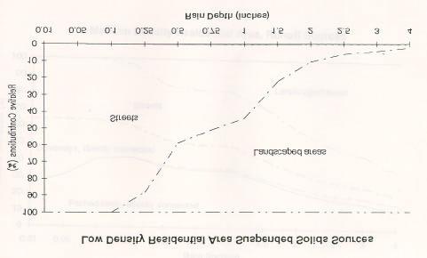
80 5-80

81 5-81

82 5-82

83 5-83

84 WinSLAMM Calibration Procedures The calibration and verification procedures of WinSLAMM are similar to the procedures needed to calibrate and verify any stormwater quality model. Local data should be collected, including stormwater outfall quality and quantity data and watershed information. Numerous individual rainfall-runoff events need to be sampled (using flowweighted composite sampling). The best scenario is to collect all calibration information from one watershed and then verify the model using independent observations from another watershed. Another common approach is to collect calibration information for a series of events from one watershed, and then verify the calibrated model using additional data from other storms from the same watershed. 5-84