Disclaimer. Readme. Red text signifies a link.

Transcription

1 Disclaimer This is a scanned reproduction of the original document for distribution purposes via electronic format. Effort has been made to provide an accurate and correct document. The document is supplied "as-is" without guarantee or warranty, expressed or implied. A hard copy of the original can be provided upon request. Readme The following will be consistent throughout the documents distributed by the Center for Subsurface Modeling Support via Acrobat Reader: C C C Red text signifies a link. Bookmarks have been developed and will vary from document to document and will usually include table of contents, figures, and/or tables. Most figures/graphics will be included at the end of the document.

2 . EPA/600/R-93/010 February 1993 A MANUAL OF INSTRUCTIONAL PROBLEMS FOR THE U.S.G.S. MODFLOW MODEL by Peter F. Andersen GeoTrans, Inc Manekin Plaza, Suite 100 Sterling, Virginia DYNAMAC CONTRACT 68-C Project Officer John E. Matthews Extramural Activities and Assistance Division Robert S. Kerr Environmental Research Laboratory Ada, Oklahoma ROBERT S. KERR ENVIRONMENTAL RESEARCH LABORATORY OFFICE OF RESEARCH AND DEVELOPMENT U. S. ENVIRONMENTAL PROTECTION AGENCY P.O. BOX 1198 ADA, OKLAHOMA ~ Printed on Recycled Paper

3 DISCLAIMERS The information in this document has been funded in part by the Environmental Protection Agency under DYNAMAC Contract No. 68-C with GeoTrans Inc. as a sub-contractor. Scott Huling and Randall ROSS, Robert S. Kerr Environmental Research Laboratory, will serve as Task Managers on this project. It has been subject to the Agency's peer and administrative review, and it has been approved as an EPA document. Mention of trade names or commercial products does not constitute endorsement or recommendation for use. This report utilizes the U.S.G.S. Modular Three-Dimensional Ground-Water Flow Model (MODFLOW) for analyzing groundwater flow under various hydrologic conditions. MODFLOW is a public-domain code and may be used and copied freely. If errors are found in the document or if YOU have suggestions for improvement, please contact the Center for Subsurface Modeling Support (CSMOS) at the Robert S. Kerr Environmental Research Laboratory, Ada, Oklahoma. Center for Subsurface Modeling Support Robert S. Kerr Environmental Research Laboratory P.O. Box 1198, Ada, Oklahoma (405)

4 FOREWORD EPA is charged by Congress to protect the Nation s land, air and water systems. Under a mandate of national environmental laws focused on air and water quality, solid waste management and the control of toxic substances, pesticides, noise and radiation, the Agency strives to formulate and implement actions which lead to a compatible balance between human activities and the ability of natural systems to support and nurture life. The Robert S. Kerr Environmental Research Laboratory is the Agency s center of expertise for the investigation of the soil and subsurface environment. Personnel at the Laboratory are responsible for the management of research programs to: (a) determine the fate, transport and transformation rates of pollutants in the soil, and the unsaturated and saturated zones of the subsurface environment (b) define the processes to be used in characterizing the soil and subsurface environment as a receptor of pollutants; (c) develop techniques for predicting the effects of pollutants on ground water, soil, and indigenous organisms; and (d) define and demonstrate the applicability and limitations of using natural process, indigenous to the soil and subsurface environment for the protection of this resource. EPA is involved in groundwater flow modeling to analyze and predict the movement of water in the subsurface. Traditionally, groundwater flow models are rarely supported by documents that assemble the practical application aspects of modeling. While it is important to understand the theory behind the mathematical model, it is equally important to understand the principles of modeling, model options, rules of thumb, and common mistakes from an applications perspective. This manual was developed specifically for the U.S.G.S. modular groundwater flow model (MODFLOW) and it illustrates by examples, the principles of groundwater flow modeling and model options. The manual was developed to be used for self-study or as a text for courses. Three diskettes are included which contain the input and output data sets for each problem presented in the manual. A copy of the MODFLOW code is not included. The information in this document should be of interest to both the beginner and advanced modeler for hands-on experience with the practical application of MODFLOW. Clinton W. Hall Director Robert S. Kerr Environmental Research Laboratory iii

5 I

6 CONTENTS Foreword... iii Figures... iv Tables... vii Acknowledgment... ix Introduction... I-1 The Theis solution Anisotropy Artesian-water table conversion Steady-state Mass balance Similarity solutions in calibration Superposition Grid and time stepping considerations Calibration and prediction Transient calibration Representation of aquitards Leaky aquifers Solution techniques and convergence Head dependent boundary conditions Drains Evapotranspiration Wells Cross-sectional simulations Application to a water supply problem Application to a hazardous waste problem References...R-1 Appendix A: Abbreviated Input Instructions for MODFLOW... A-1

7 FIGURES Number I Configuration of the model for simulating radial flow Parts a-d Drawdown versus time for each model configuration Drawdown versus time at the observation point located 55 m from the pumping well along the x-axis for the three model configurations Drawdown versus time at the observation point located 55 m from the pumping well along the y-axis for the three model configurations Drawdown contours (ft) for the 10:1 anisotropic case modeled in Part a Three-dimensional view of the drawdown for the 10:1 anisotropic case modeled in Park a Drawdown versus time for the four MODFLOW configurations and the analytical solution Drawdown versus distance at 2.19 days for the water table, conversion, and artesian cases Configuration of the Problem 4 modeled domain Potentiometric surface map and hydraulic head array at time step Model wide mass balance at time step l Printout of cell-by-cell flow terms for each component of the mass balance Hand calculations for each component of the mass balance Contour map of potentiometric surface, hydraulic head may, and mass balance output for Part a Contour map of potentiometric surface, hydraulic head array, and mass balance output for Part b Contour map of potentiometric surface, hydraulic head array, and mass balance output for Part c Contour map of potentiometric surface, hydraulic head array, model wide mass balance, and individual specified head node mass balance for Park a Contour map of potentiometric surface, hydraulic head array, model wide mass balance, and individual specified head node mass balance for Part b Contour map of potentiometric surface, hydraulic head array, model wide mass balance, and individual specified head node mass balance for Part c Contour map of potentiometric surface, hydraulic head array, model wide mass balance, and individual specified head node mass balance for Pare d Location of pumping wells, observation wells, and boundary ) conditions for Problem page vi

8 Drawdown (m) at 20 days for the 4 x 4 grid simulation of Part a Drawdown (m) at 0.2 days for the 16x 16 grid simulation of Part b Geometry and potentiometric surface of the aquifer system Hydraulic head arrays, potentiometric surface contour maps, and mass balance summary for Part a Hydraulic head arrays, potentiometric surface contour maps, and mass balance summary for Part b using pumpage of -0.4 ft 3 /s Potentiometric surface contour map for Part b using pumpage of -0.1 ft 3 /s Potentiometric surface contour map for Part b using pumpage of -0.5 ft 3 /s l0 Grid and boundary conditions for coastal transient problem Hydraulic head (ft) in the middle of the confining bed versus time for ll-5cases a, b, and d Total flux (ft 3 /s) and storage flux versus time from the confining bed for the seven layer model Drawdown versus time for the analytical, MODFLOW, and SEFTRAN simulations Model geometry, boundary conditions, and hydraulic conductivity zonation for Problem Iteration history for variations in the SIP seed parameter Iteration history for variations in the SSOR acceleration parameter Hydraulic head (ft) versus flow rate (ft 3 /d) for each of the five methods of representing the third type boundary conditions Model configuration for Problem Finite-difference grid, boundary conditions, and simplified topography for Problem Potentiometric surface (ft) for Problem 16, Part a Potentiometric surface (ft) for Problem 16, Part b (net recharge) Drawdown map (ft) for Problem 16, Part c Drawdown (ft) map for Problem 16, Part d Net recharge rates (in/yr) for the steady-state, non-pumping scenario (part a) Drawdown versus distance for the fully penetrating well case and the partially penetrating well case in the 20 m thick aquifer at time = s Drawdown versus distance for the fully penetrating well case and the partially penetrating well case in the 40 m thick aquifer at time = s Layering and zonation used in the cross-sectional model Hydraulic head arrays for the cross-sectional model Geologic map of the Musquodoboit harbor region Geologic map of the Musquodoboit harbor region Model boundary and transmissivity zones used in the numerical model Location of the river boundary condition, pumping well, and observation wells used in the numerical model vii

9 a 20.3b 20.3c 20.3d 20.4 Drawdown (ft) versus time (min) for the aquifer test conducted at Musquodoboit Harbor Comparison of modeled to observed drawdown (ft) data for the base case Comparison of modeled to observed drawdown in well 1 for the base case and for a 2-fold increase and reduction in transmissivity Comparison of modeled to observed drawdown in wells for the base case and for storage coefficients of 0.1 and Drawdown (ft) after 1000 days of pumping at ft 3 /s Comparison of modeled drawdown for the drawdown dependent Storage Coefficient Comparison of modeled to observed drawdown in well 1 for the base case and for order of magnitude increase and decrease in river conductance Finite difference grid showing the location of specified head cells for the steady-state model Grid cells representing the impermeable clay cap, the slurry wall, and the drain Hydraulic head (ft) contours in the vicinity of the landfill for the steady-state case (a) Hydraulic head (ft) contours in the vicinity of the landfill for the case involving a cap (b) Hydraulic head (ft) contours in the vicinity of the landfill for the case involving a cap and a slurry wall (c) Hydraulic head (ft) contours in the vicinity of the landfill for the case involving a cap and a drain (e) Hydraulic head (ft) along column 19 of the model at 2.69 years for each remedial alternative simulation viii

10 Number Page Verification of MODFLOW results i-4 Packages used in the problem sets I-5 Parameters used in Problem l Grid spacing (m) used for various model configurations Calculations for determination of transmissivity and storage coefficient for wedge-shaped domain Drawdown versus time for each model configuration Parameters used in Problem Grid spacing used in the various model configurations Drawdown (m) at an observation point located 55 m from the pumping well along the x axis Drawdown (m) at an observation point located 55 m from the pumping well along they axis Drawdown (m) at an observation point located 77.8 m from the pumping well at a 45 0 angle between the x and y axis Parameters used in Problem Grid spacing (ft) used in Problem Drawdown versus time for each model configuration Initial head (SHEAD) at specified head cells Hydraulic head (ft) at node (7,1), storage component of mass balance, and iteration data for each time step and the steady-state simulations Comparison of model calculated and hand calculated rate mass balance Grid data Comparison of results for various grid spacings in Part a Comparison of results for various grid spacings in Part b Comparison of results for variations in time stepping in Part c Comparison of results for variations in closure criterion in Part d Comparison of drawdowns (m) at well 2 for various time derivatives and spatial approximations (analytical = 1.63) River data Calibration targets Hydraulic head (ft) versus time (weeks after drought began) at an observation well located at node (1,5) Pre-drought groundwater levels (ft) within the model domain Groundwater levels resulting from a steady-state simulation using a hydraulic conductivity of 850 ft/d Hydraulic heads (ft) in the middle of the confining bed versus time for all cases of Problem 1l Parameters and discretization data used in Problem ix

11 Time versus drawdown (analytical solution) at distances of m Time versus drawdown at distances of m for the analytical solution, MODFLOW configuration, and SEFTRAN radial solution Sensitivity analysis on SIP seed and acceleration parameter Sensitivity analysis on SSOR and acceleration parameter Aquifer parameters and discretization data for Problem Hydraulic head at node (1,4) for each of the five methods of representing the third type boundary condition Discharge for each of the five methods of representing the third type boundary condition Other uses for the head-dependent flux boundary conditions in MODFLOW Grid spacing used in the fine-gridded model (Part b) Hydraulic head at the drain node (column 6) and drain flux for variations in drain conductance (coarse model) Comparison of hydraulic heads (ft) along row 10 for MODFLOW and FTWORK Parameters and discretization used in Problem Drawdown versus distance at s for the fully penetrating, partially penetrating, and stratified aquifer simulations Bottom and top elevations (ft) in cross-sectional model Initial heads inlayer Assumed saturated thickness (ft) of layer 1 in the cross-sectional model Input data for the water supply problem Observed drawdown data from aquifer test Modeled drawdown data for the base case Drawdown (ft) versus time in observation well 1 for variations in transmissivity, storage coefficient and river leakance Attributes of the drain used in Part d Comparison of MODFLOW results versus USGS2D results for the steady-state case (part a) and the wall and cap scenario (Part c) at 6.08yr Hydraulic heads (ft) along column 19 of the model at 2.69 years for each remedial alternative simulation Drain discharge (ft 3 /s) versus time for the well, cap, and drain scenario (part d) and the cap and drain scenario (part e)

12 ACKNOWLEDGMENTS The author wishes to thank the many individuals who have contributed to make this document possible. In particular, I thank Joanne Elkins of GeoTrans, Inc. who was largely responsible for typing this document. Also, I wish to thank Debbie Shackleford and Carol House of Dynamac Corporation for the final preparations of the document. Finally, I thank my students at the International Ground Water Modeling Center s (IGWMC) Applied Groundwater Modeling short course for their many helpful suggestions. xi

13 I

14 INTRODUCTION A recent report by the United States Environmental Protection Agency Groundwater Modeling Policy Study Group (van der Heijde and Park, 1986) offered several approaches to training Agency staff in the application of groundwater modeling. They identified the problem that current training efforts tend to be of short duration (one week or less) with a lack of in-house programs to reinforce training received in a formal setting. The study group suggested, among other things, the alternative of self-study coupled with obtaining experience under the guidance of a senior modeling specialist. In order for groundwater modeling self study to be viable, a curriculum must exist that allows the student to have hands-on experience with the practical application of models. Available resources do not meet this need. Current groundwater modeling texts deal primarily with the mathematics or theory of modeling. Code documentations usually discuss the programming aspects and performance standards of particular models. They usually include one or two test problems for verification purposes. Journal articles or U.S. Geological Survey publications best fit the need for learning about the practical application of models. However, these sources either do not give enough information to reproduce results or involve data setup that is too complicated to allow a student to efficiently have hands-on experience with the model. This manual is intended to meet the need described above. Twenty documented problems, complete with problem statements, input data sets, and discussion of results are presented. The problems are designed to cover modeling principles, specifics of input/output options available to the modeler, rules of thumb, and common modeling mistakes. Data set preparation time and execution time have been minimized by simplifying the problems to small size and to focus only on the aspect that is under consideration. Model grids are generally smaller and more homogeneous than would be used in practice, however, the intent and result of each exercise are not compromised by the simplification. This manual is developed for the U.S. Geological Survey modular groundwater model (MODFLOW) by McDonald and Harbaugh (1988). MODFLOW is perhaps the most popular groundwater flow model used by government agencies and consulting fins. MODFLOW solves the partial differential equation describing the three-dimensional movement of groundwater of constant density through porous material: (1.1) I-1

15 where: are values of hydraulic conductivity along the x, y, and z coordinate axes, which are assumed to be parallel to the major axes of hydraulic conductivity (LT -1 ); h W S s t is the potentiometric head (L); is a volumetric flux per unit volume and represents sources and/or sinks of water (T -l ); is the specific storage of the porous material (L l); and is time (T). S s, K xx, K yy, K zz, may be functions of space and W may be a function of space and time. This equation, combined with specification of boundary and initial conditions, is a mathematical expression of a groundwater flow system. MODFLOW uses the finite difference method to obtain an approximate solution to this equation. Hydrogeologic layers can be simulated as confined, unconfined, or a combination of confined and unconfined. External stresses such as wells, areal recharge, evapotranspiration, drains and streams can also be simulated. Boundary conditions include specified head, specified flux, and head-dependent flux. Two iterative solution techniques, the Strongly Implicit Procedure and Slice Successive Over Relaxation, we contained within MODFLOW to solve the finite difference equations (McDonald and Harbaugh, 1988). The user of this manual should attempt to solve the problems as described in the problem statement portion of each exercise. The model setup can be checked in the data set listing given in the model input section of each problem. Results can be checked by the pertinent portions given in the model output section. Some training on the structure and input of MODFLOW as well as some training on the theory of groundwater modeling is assumed. The user will need to refer to the MODFLOW manual on some occasions. The abbreviated input instructions given in the MODFLOW manual are included as Appendix A to this manual. A secondary function of this manual is for verification purposes. Although the MODFLOW code has been extensively applied, very little documentation of its testing and verification is available in the literature. To address this situation, where possible, model generated results are compared to analytical solutions, results of other models, or to simulations with alternative boundary conditions or configurations. In addition to providing an informal benchmarking of MODFLOW, these problems can be used to verify the correct installation of the code on a particular computer system or to verify that certain user modifications have not altered the integrity of the program. The results of the simulations may vary slightly (approximately dl.02 ft or m) from one computer to another. The results obtained here were with a 386 microcomputer. Table 1 shows the problems that were run and what types of verification were performed. I-2

16 All the packages of MODFLOW have been utilized at least twice in this series of problems. Table 2 is a matrix showing which packages were utilized in individual problems. Several parts exist to each problem. Input and output files are included on the attached diskette for the data sets listed in the manual. Minor modifications, as described in the model input section of each problem are not included as separate data sets. The diskettes included with this document do not include a copy of MODFLOW. It is assumed the reader has obtained a copy of MODFLOW and has the necessary computer hardware to execute the program. The problems given in the manual are intended to be useful without changes or additions. However, the problems may also be useful as a stepping stone to more detailed analysis. Rather than creating new data sets, the analyst can modify existing data sets to fill a particular need. I-3

17 Table 1. Verification of MODFLOW results Alternate Boundary Analytical or Condition or Problem Semianalytical Numerical Model No. Title Solution Model Configuration 1 Theis solution X Anisotropy Artesian-water table conversion Steady State Mass balance Similarity solutions in model calibration Superposition Grid and time stepping considerations Calibration and prediction Transient calibration Representation of aquitards Leaky aquifers Solution techniques and convergence Head dependent boundary conditions Drains Evapotranspiration Wells Cross-sectional simulations Application to a water supply problem Application to a hazardous waste site x x X X X X X X X x x X X X I-4

18 1 Table 2. Packages used in the problem sets* Problem output No. Well Drain River ET GHB Recharge SIP SSOR Control 1 x x x 2 x x x 3 x x x 4 x x x x 5 x x x 6 x xx x 7 x x x 8 x x x 9 x x x x 10 x x x 11 x x 12 x x x 13 x x x 14 x x x x x x x 15 x x x 16 x x x x 17 x x x 18 x x x x x x x x x x x x *The Basic and Block Centered Flow packages were used for all simulations. Packages available in MODFLOW and their major function am: Basic Block Centered Well Drain ET GHB Recharge SIP SSOR Output Control River Flow Overall model setup and execution Calculates terms of finite difference equations for flow within porous media Specified flux condition (volumetric input) Head dependent flux condition limited to discharge Evapotranspiration, head dependent flux condition limited to discharge with a maximum specification of discharge General Head Boundary, head dependent flux condition Specified flux condition (linear input) Strongly Implicit Procedure solution technique Slice Successive Over Relaxation solution technique Directs amount type, and format of model output River flux condition I-5

19

20 PROBLEM 1 The Theis Solution INTRODUCTION With the exception of Darcy s Law, perhaps the most widely used analytical technique by hydrologists is the solution by Theis (1935). It is therefore fitting that the first problem presented in this manual is a benchmark of MODFLOW with the Theis solution. Three different model configurations for analyzing radial flow to a well are examined. The techniques described in this problem can be generally applied to well test analysis and representations of radial flow. PROBLEM STATEMENT AND DATA Theis solution predicts drawdown in a confined aquifer at any distance from a well at any time since the start of pumping given the aquifer properties, transmissivity and storage coefficient. The assumptions inherent in the Theis solution include: 1) The aquifer is homogeneous, isotropic, uniform thickness, and of infinite areal extent. 2) The initial potentiometric surface is horizontal and uniform. 3) The well is pumped at a constant rate and it fully penetrates the aquifer. 4) Flow to the well is horizontal, the aquifer is fully confined from above and below. 5) The well diameter is small, storage in the wellbore can be neglected. 6) Water is removed from storage instantaneously with decline in head. All of these assumptions, with the exception of infinite areal extent can be easily represented with the numerical model. Several options exist to represent the domain as effectively infinite. The most frequently applied method is to extend the model domain beyond the effects of the stress. The modeled domain is therefore usually fairly large and a limited time frame is modeled. An increasing grid spacing expansion is used to extend the model boundaries. The model domain is assumed to be uniform, homogeneous, and isotropic. A single layer is used to model the confined aquifer. A fully penetrating well located at the center of the model domain pumps at a constant rate. The potentiometric surface of the aquifer is monitored with time at an observation well 55 m from the pumping well. Specific details of the problem are from Freeze and Cherry (1979) pp. 345, and are given in Table

21 I Table 1.1. Parameters used in Problem 1 Initial head Transmissivity Storage coefficient Pumping rate Final time Number of time steps Time step expansion factor SIP iteration parameters Closure criterion Maximum number of iterations 0.0 m m 2 /s x 10 3 m 3 /s S Part a) Represent the entire aquifer domain by using the grid spacing shown in Table 1.2. Place the well at the center of the domain, row 10, column 10. Run the model, noting drawdown at each time step at an observation point 55 m from the pumping well. The configuration of the model for part a and future parts b, c, and d is shown in Figure 1.1. ) 1-2

22 Table 1.2. Grid spacing (m) used for various model configurations Part a Part b Part c Row number, i DELC (i) DELC(i) DELC(i) (=column number, j) (=DELR(j)) (=DELR(j)) (=DELR(j))

23 Figure 1.1. Configuration of the model for simulating radial flow for parts ad. Arrows denote groundwater flow direction. Part b) Part c) Part d) Because of symmetry, the aquifer domain can be represented as a quadrant. Set up a second model covering only the lower right quadrant of the previous domain. The grid spacing for this model is shown in Table 1.2. Position the well at the upper left comer of the new model, row 1, column 1. Because only one-fourth of the aquifer is simulated, the well discharge should also be reduced to one-fourth the original discharge. Run the model and note drawdown at each time step at an observation point 55 m from the pumping well. Re-run part b with the grid spacing shown in Table 1.2. The overall model domain is the same size as part b, but grid spacing is finer near the pumping well. Run the model and note drawdown at each time step at an observation point 55 m from the pumping well. Another form of symmetry for this problem (radial flow) is a pie shaped wedge with the well at the vertex of the wedge. Unfortunately this geometry is difficult to represent because the finite difference method is based on orthogonality of rows and columns. However, because the model is posed in terms of conductance (a

24 function of grid spacing and transmissivity) and grid block storativity (a function of storage coefficient and area) it is possible to adjust T and S in such a manner to approximate the wedge. Using a 20 m wide row (DELC( 1) = 20) and grid spacing along a row (DELR) as in part b, calculate changes to transmissivity and storage coefficient for a 10 pie wedge. Adjust the well discharge to account for the reduced model domain and input these parameters into the model. Run this one-dimensional model and note drawdown at each time step at an observation point 55 m from the well. 1-5

25 MODEL INPUT The following is a listing of data sets used for part a 1-6

26 The same data set was used in part b, except the model domain was reduced to a 10x10 grid (NROW = 10, NCOL =10) in the BASIC package. Accordingly, only one-fourth of the grid, (as shown in Table 1.2, part b) was used. In addition, the well discharge was moved to row 1, column 1 and reduced to lx10-3 m 3 /s in the WELL package. The part c data set is identical to part a, except grid spacing (DELC, DELR in the BCF package) is modified as shown in Table 1.2 and the well location and discharge is as in part b. The data set for part d is shown below, minus the SIP and output control files, which are identical to those of parts a-c. The calculations for adjustment to transmissivity and storage coefficient are shown in Table

27 I Table 1.3. Calculations for determination of transmissivity and storage coefficient for wedge-shaped domain (part d) 10 arc Area Individual Wedge length DELC block area area Radius to Ẏ Block x Radius to of 10 * block 10 arc actual number j DELR block edge wedge actual area midpoint length DELC Adjusted transmissivity = 10 arc length * transmissivity actual DELC Adjusted storage coefficient = wedge area * storage coefficient actual area 1-8

28 MODEL OUTPUT Drawdowns versus time are tabulated in Table 1.4 for each of the four cases. Comparison is also made to the analytical solution of Theis. A drawdown versus time plot is shown in Figure 1.2 for the best comparison case (the refined quadrant) and the worst comparison case (the coarse quadrant). Other cases are not shown, but are generally very similar to the refined quadrant case. Table 1.4. Drawdown versus time for each model configuration Time Step Time (see) Analytic Drawdown (m) Refined Full grid (case a) Quadrant (case b) Quadrant (case c) Pie Wedge (case d)

29 . With the exception of the coarse quadrant grid (case b), the MODFLOW results compare well to the analytic solution. The numerical results are generally within m of the analytic. An exact comparison is not attained because of the approximations made in the numerical model. These include: 1) use of a discrete rather than continuous spatial domain, 2) use of a discrete rather than continuous time domain, 3) use of an iterative solution with a closure tolerance, and 4) artifical placement of boundaries. The distant no-flow boundary is only a small factor in this analysis because it is placed far enough from the stress so that drawdown at the boundary is very limited. There is a significant departure from the Theis curve at the final time step, however, as the non-infinite nature of the model domain becomes a factor. The comparison would continue to deteriorate if the model were run for longer time. 1-10

30 This problem illustrates three methods of modeling radial flow to a well. The first placing the well at the center of a rectangular grid, is the most intuitive approach to this problem, but is not the most efficient. The second method, the quadrant recognizes symmetry of flow. Some care must be taken in designing the grid. The third method, the pie wedge, also recognizes symmetry but involves fairly labor intensive parameter adjustment to approximate a wedge shaped grid. The quadrant grid is a satisfactory approximation, provided it is sufficiently fine near the pumping well. The predominant reason for the approximation error noted in the first quadrant analyzed (case b) is because the block-centered grid approach models a larger area than a quadrant. There will always be an extra 1/2 grid block on the margins of the model area and therefore extra storage in the model domain. The extra storage accounts for a majority of the underprediction of drawdown in case b. When the size of the blocks on the margins is reduced in case c, the error is also reduced. The pie-wedge grid provides a reasonable approximation for this particular problem. The user is cautioned that it is conceptually difficult and error-prone to develop the grid and aquifer parameters for this type of configuration. Some approximation errors may become more apparent if larger areas or greater wedge angles are used. Although this is an appropriate methodology, its main reason for presentation in this manual is to reinforce the user s understanding of the relationship between transmissivity, grid spacing, and conductance. 1-11

31

32 PROBLEM 2 Anisotropy INTRODUCTION Anisotropy is often encountered in aquifers, particularly in the vertical direction. Vertical anisotropy is handled in MODFLOW through the VCONT term, which is used in the threedimensional simulations. Horizontal anisotropy can also occur and may result from fracture networks or depositional environments. Although MODFLOW was designed as a porous media model, the scale of many modeling efforts is such that fractured media or a karst environment can be considered an equivalent porous media. This problem examines how MODFLOW handles horizontal anisotropy, provides a check on model accuracy, and illustrates some special considerations for modeling anisotropic aquifers. PROBLEM STATEMENT AND DATA This problem is very similar to the Theis problem (problem 1) with regard to assumptions, model configuration, and hydraulic parameters. An effectively infinite confined aquifer is assumed, with a fully penetrating well located at the center of the model domain pumping at a constant rate. The aquifer is ten times as transmissive in the x-direction as in the y direction. For parts a and b, the principal directions of the hydraulic conductivity tensor are assumed to be aligned with the model grid. The potentiometric surface of the aquifer is monitored at 3 points: 55 m from the pumping well in the x direction, 55 m from the pumping well in the y direction, and 77.8 m from the pumping well along a diagonal at 45 to the x and y axis. Specific details on the problem are nearly identical to the Theis problem and are given in Table 2.1. The data sets from problem 1 can be easily motified rather than creating new data sets. Note that areal anisotropy is handled with the TRPY term in the BCF package. 2-1

33 Table 2.1. Parameters used in Problem 2 Initial head Transmissivity, T xx Transmissivity, T yy Storage coefficient Pumping rate Stress period length Number of time steps Time step expansion factor SIP iteration parameters Closure criterion Maximum number of iterations 0.0 m m 2 /s m 2 /s x 10-3 m 3 /s S Part a) Represent the entire aquifer domain with the grid spacing shown in Table 2.2. Note that this spacing is the same as problem 1, part a. Place the well at the center of the domain, row 10, column 10. Run the model, noting drawdowns at each time step at the 3 observation points described above. 2-2

34 Table 2.2. Grid spacing used in the various model configurations Part a Part b Row number, i DELC(i) DELC(i) (=column number,j) (=DELR(j)) (=DELR(j)) Part b) Part c) Represent a quadrant of the aquifer domain with the grid spacing shown in Table 2.2. Note that this is the same spacing used in problem 1, part c. Place the well at the upper left comer of the model, row 1, column 1 and reduce the pumping to onefourth the original value. Note drawdowns at each time step at the 3 observation points. In the previous parts to this problem, the principal directions of the hydraulic conductivity tensor were aligned with the finite difference grid. That is, the maximum T ( m 2 /s) was along the x axis while the minimum T ( m 2 /s) was along the y axis. In this exercise, we will examine the error which occurs if the grid is not aligned with the principal directions of the hydraulic conductivity tensor. We will assume that the maximum T is still m 2 /s and the minimum T is still m 2 /s and at right angles to one another, however, the analyst has not aligned the finite difference grid along these maximums and minimums. The grid is tilted 2-3

35 20 off the principal directions of hydraulic conductivity. The transmissivity along the x and y axis can be calculated from equations given by Bear (1972), page 140. (2.1) (2.2) Solving equations 2.1 and 2.2 gives T xx = m 2 /s T yy = m 2 /s an additional term, called a cross product term, is introduced: (2.3) solving equation 2.3 gives T xy = m 2 /s Note that T xy is larger than T yy. Using the grid from part a input the transmissivities calculated above into the BCF package. Because the grid alignment is assumed to coincide with the principal directions of hydraulic conductivity, MODFLOW does not accommodate T xy. Therefore, for the purposes of this exercise, it is ignored. Run the model and note drawdown versus time at each of the three observation points. 2-4

36 I MODEL INPUT The following is a listing of the input data sets for part b. 2-5

37 Part b is shown here because part a is nearly identical to that of problem 1, part a which was shown previously in the problem 1 writeup. The only difference between the previous part a data set and the current part a data set is that the layer wide anisotropy ratio (TRPY) is changed from 1.0 to 0.1 to yield a transmissivity along a column of1/1o that along a row. The part b data set shown above is nearly identical to that of part c of Problem 1. Again the layer wide anisotropy ratio is set at 0.1 for the current simulation. In part c, the same data set as part a is used, however, the transmissivity along a row (TRAN) is changed to m 2 /s. Because we desire a transmissivity of m 2 /s along the y axis (column), the layer wide anisotropy ratio is set at / or MODEL OUTPUT Drawdown versus time is tabulated for the three observation points in Tables 2.3, 2.4, and 2.5 for the three cases. These results may be compared to the analytical solution of Papadopulos (1965) for anisotropic aquifers. The results of these simulations are plotted in Figures 2.1 and

38 Table 2.3. Drawdown (m) at an observation point located 55 m from the pumping well along the x axis Drawdown (m) Time step number Time (see) Analytic Part a Part b Part c

39 . - Table 2.4. Drawdown (m) at an observation point located 55 m from the pumping well along they axis Time step number Drawdown (m) Time (see) Analytic Part a Part b Part c

40 Table 2.5. Drawdown (m) at an observation point located 77.8 m from the pumping well at a 45 angle between the x and y axis Drawdown (m) Time step number Time (see) Analytic Part a Part b Part c

41 Figure 2.1. Drawdown versus time at the observation point located 55 m from the pumping well along the x-axis for the three model configurations. 2-1o

42 Figure 2.2. Drawdown versus time at the observation point located 55 m from the pumping well along the y-axis for the three model configurations. 2-11

43 DISCUSSION OF RESULTS The comparison of MODFLOW results with the analytical solution is again very good. However, just as the overall grid design was important in the Theis problem, the directional grid design becomes important for areally anisotropic problems. Note in Figures 2.3 and 2.4 that the drawdown contours form an ellipse with the major axis in the direction of highest transmissivity. The model results are in excellent agreement with analytical results along the y-axis, which is in the direction of low transmissivity, for both the coarse and fine grids (see Table 2.4 and Figure 2.2 for parts a and b). It appears from these results that the coarse and fine grids are equally satisfactory. Along the x-axis, or direction of high transmissivity, there is a more apparent difference between the results of the coarse and fine meshes. The results using the fine mesh are very close to the analytical results, but the coarse mesh results consistently show greater drawdown. This is not a boundary effect the model boundary is located at equivalent distances (1000 m) for both grids. Instead, the grid resolution influences the results more in this direction because the drawdown and gradient to the pumping well are greater than in the y-direction. This illustrates that for areally anisotropic problems, grid design becomes even more important than for isotropic problems. As a general rule for all models, grids should be designed to match expected gradients. The grid should be able to accommodate the vertical curvature of streamlines. Note that the results along the 45 angle (Table 2.5) are similar to the results along the y-axis and are therefore not plotted. The coarse and fine grids are also equally effective in providing satisfactory answers. Inspection of Figure 2.3 shows the similarity between the results along the y-axis and along the 45 angle. The results of part c, where the grid was not aligned with the principal directions of the hydraulic conductivity tensor, shows significant deviation from the analytical results. Note that MODFLOW does not have the capability to accurately model a situation such as this. The principal directions of the hydraulic conductivity tensor must be aligned with the x and y directions of the model grid. Even a small misalignment 20 in case c, can cause significant errors. This becomes even more apparent for highly fractured systems where anisotropy ratios may be greater than 10:1. Areal anisotropy is handled in MODFLOW by the TRPY term, which establishes the ratio of transmissivity along a column to transmissivity along a row. Note that this is a layer wide term and a given anisotropy ratio is therefore assumed to exist layer wide. 2-12

44 Figure 2.3. Drawdown contours (ft) for the 10:1 anisotropic case modeled in part a 2-13

45 Figure 2.4. Three-dimensional view of the drawdown for the 10:1 anisotropic case modeled in part a 2-14

46 PROBLEM 3 Artesian-water table conversion INTRODUCTION When a confined aquifer is heavily stressed, its potentiometric surface may be drawn down sufficiently such that the aquifer begins to dewater. or behave as a water-table aquifer. This conversion takes place when the potentiometric surface falls below the top of the aquifer. The primary change that takes place in a situation such as this is with the storage coefficient (s); under confined conditions water is derived from pressure changes and S is fairly small, while under water-table conditions water is derived from dewatering pore spaces and S is usually fairly large. A secondary change is that if drawdown is sufficient to cause changes in saturated thickness, the transmissivity of the aquifer will be reduced. MODFLOW has the capability to model both these effects. This problem demonstrates the physical process of the conversion, how it is implemented in MODFLOW simulations, and compares the numerical results to an analytical solution. PROBLEM STATEMENT AND DATA The problem is essentially the same as the example presented by Moench and Prickett (1972) who derived an analytical solution to the artesian-water-table conversion problem. The assumptions inherent in the Theis solution are also a part of this solution. Of particular interest to this problem, the thickness of the aquifer is assumed to be such that the dewatering does not significantly reduce the aquifer transmissivity, all flow lines in the water table region are assumed horizontal, and water is released instantaneously from storage. The model domain is assumed to be effectively infinite; the grid is therefore extended to where the effects of the stress are negligible. A fully penetrating well located at the center of the aquifer pumps at a constant rate. The potentiometric surface of the aquifer is monitored with time at an observation well 1000 ft from the pumping well. Specific details on the problem are given in Table 3.1 and are from Moench and Prickett (1972). 3-1

47 Table 3.1. Parameters used in Problem 3 Initial head Transmissivity Storage coefficient (confined) Specific yield (unconfined) Pumping rate Stress period length Number of time steps Time step expansion factor SIP iteration parameters Closure criterion Maximum iterations 0.0 ft ft2/d O ft3/d 100 days Part a) Part b) Part c) Represent the entire aquifer domain by using the grid spacing shown in Table 3.2. Place the well at node 1,1, and use one-fourth of the well discharge given in Table 3.1, because only 1/4 of the aquifer domain is modeled. Place the aquifer top at -1 ft. Use layer type 2 (LAYCON) so that the conversion only involves a change in storage coefficient. Run the model and note drawdown with time at a point 1000 ft from the pumping well. Run the problem with the aquifer top set at -2 ft. Note drawdown versus time at a point 1000 ft from the pumping well. Compare to part a Run the problem as confined (LAYCON = O) with storage coefficient of and note drawdown versus time at a point 1000 ft from the pumping well. Part d) Rerun part c except use a storage coefficient of 0.1 and note drawdown at a point 1000 ft from the pumping well. versus time 3-2

48 Table 3.2. Grid spacing (ft) used in Problem 3 Row number i (=column number, j) DELC(i) (=DELR(j)) O

49 MODEL INPUT The following is a listing of the input data sets for part a 3-4

50 3-5

51 . In part b, aquifer top ( TOP) is set to -2 ft. In part c layer type (LAYCON) is changed to O. As a result the secondary storage factor (SF2) and aquifer top (TOP) are no longer required. In part d, the primary storage factor (SFI) is changed from to 0.1. MODEL OUTPUT Drawdown versus time is tabulated in Table 3.3 and plotted in Figure 3.1 for each of the four cases. The results of parts a and b can also be compared to Moench and Prickett (1972) which is reproduced on the table. Table 3.3. Drawdown versus time for each model configuration Drawdown (ft) Aquifer top at -1 ft Aquifer top at -2 ft Time step number Time (days) Confined Unconfined Analytical MODFLOW Analytical MODFLOW S= S= % ,

52 Figure 3.1. Drawdown versus time for the four MODFLOW configurations and the analytical solution. DISCUSSION OF RESULTS This problem demonstrates the physical process of artesian/water table conversion as related to the change in storage coefficient. MODFLOW results compare well to the analytical results for both locations of aquifer top datum. It is apparent from Figure 3.1 that the time-drawdown plots for the conversion cases are enveloped between the artesian and water-table time-drawdown plots. The greater the distance from the initial potentiometric surface to the aquifer top, the closer the curve becomes to the artesian case. The shape of the curve is generally similar prior to conversion to the Theis curve for artesian conditions while after conversion the slope is similar to the unconfined curve. Note that the storage coefficient is only related to the time-dependent nature of drawdown. Figure 3.2 shows distance drawdown plots for the water-table, conversion, and artesian conditions at 2.19 days. Note that the conversion curve is again enveloped between the artesian and water-table curves. The water-table responds only near the well due to the large component of storage. The 3-7

53 conversion case drawdown plot shows a fairly rapid response at distance, where the aquifer is under artesian conditions. The well is,.however, obtaining much of its withdrawal from the newly squired storage in the vicinity of the well. Not shown in this exercise is the feature of MODFLOW which allows a confined aquifer transmissivity to change a saturated thickness based unconfined transmissivity. As can be seen from Figure 3.2, most of a potential change in saturated thickness would be felt immediately near the well for this problem. This is generally true for pumping well problems and it is often not necessary to incorporate this added complexity. It may be necessary to account for both storage coefficient and transmissivity conversion in relatively thin aquifers or in areas where the conversion is regional. This problem deals with artesian to water-table conversion It is also possible to convert from water-table to artesian with MODFLOW. The conversion feature may also be used in a spatial sense: parts of the model area may be under water-table conditions while others are under confined conditions. Figure 3.2. Drawdown versus distance at 2.19 days for the water table, conversion, and artesian cases. 3-8

54 PROBLEM 4 Steady-state INTRODUCTION Transient model simulations such as in the preceding problems involve flow into and out of storage within the aquifer. The preceding problems considered only wells; in complex aquifer systems other components, such as rivers, springs, evapotranspiration, and recharge, may contribute or extract flow from the system. When the aquifer is in equilibrium, flow is balanced between these various sources and sinks and the system may be in a steady-state. In this exercise, the role of aquifer storage in transient and steady state simulations is demonstrated. Several methods of simulating a steady-state solution are attempted. PROBLEM STATEMENT AND DATA The modeled domain is discretized using a seven by seven uniformly spaced finite difference grid of spacing 500 ft as shown in Figure 4.1. Specified head boundaries are located along row 1 and along column 7. These boundaries maybe conceptualized as two rivers intersecting perpendicularly in the northeastern comer of the modeled groundwater system. The hydraulic head values associated with these boundaries are given in Table 4. L Elsewhere, in the active part of the grid, use a starting head of 10.0 ft. Only a single aquifer is modeled; therefore only 1 layer is used. The aquifer is treated as confined because it is relatively thick and does not experience large changes in saturated thickness. The transmissivity of the aquifer is 500 ft 2 /d, while recharge occurs at a rate of ft/d. A well discharges at a rate of 8000 ft 3 /d at row 5, column 3. The strongly implicit procedure (SIP) solution technique is used in this exercise. The maximum number of iterations (MXITER) used is 50, the number of iteration parameters (NPARM) is 5, the acceleration parameter (ACCL) is 1.0, the head change criterion is 0.01, IPCALC = 1, WSEED = 0.0, and IPRSIP = 1. A more detailed presentation of solution techniques and convergence is presented in Problem

55 Figure 4.1. Configuration of the Problem 4 modeled domain.

56 Table 4.1. Initial heads (SHEAD) at specified head cells Row Column Head (ft) Part a) Run the model in a transient mode using a storage coefficient of Five time steps, a time step multiplier of 1.5, and stress period length of 365 days should be specified in the BASIC package. Print the mass balance (budget) and head distributions at all five time steps by using the OUTPUT CONTROL PACKAGE. Part b) Run the model in a steady-state mode by invoking that option in the BCF package. Run for 1 time step of 1 day in length. Use a time step multiplier of 1.0. Compare the results to that of part a, time step 5. Part c) Run the model in a steady-state mode as you did in part b, but run for 1 time step of 365 days in length. Compare results to that of parts a and b. Part d) Repeat part b, except use an initial head condition in the active part of the grid of 1000 ft. Compare results to that of part b. 4-3

57 MODEL INPUT The following is a listing of data sets used in problem 4 part a. In part b the time-stepping - parameters. PERLEN, NSTP, and TSMULT, are changed to 1.0, 1, and 1.0, respectively in the BASIC package. The steady state flag (lss) is changed to 1 and the storage coefficient is eliminated in the BCF package. Part c uses the part b data sets, except PERLEN, the length of the simulation, is set to 365 days in the BASIC package. Part d is identical to part b, except the initial head (SHEAD) in the active area of the model is set to 1000 ft in the BASIC package. 4-4

58 4-5

59 MODEL OUTPUT Hydraulic head, mass balance information, and iteration data are given in Table 4.2 for each simulation in this problem set. Table 4.2. Hydraulic head (ft) at node (7,1), storage component of mass balance, and iteration data for each time step and the steady-state simulations Hydraulic Into storage Out of storage Time step no. Time (days) head (7,1) (ft) (ft 3 /d) (ft 3 /d) No. of iterations Steady-state Steady-state Steady-state (initial head = 1000 ft) DISCUSSION OF RESULTS In part a, the system was run in a transient mode from an arbitrary initial condition in the active part of the model area. After 1 year of flow (recharge, pumping well, flux to constant heads, flux from constant heads, storage) the system reaches an equilibrium where heads no longer change. Flow into the system is perfectly balanced with flow out of the system. In part b, the model was run in its steady-state model (ISS = 1) for a single 1 day time step. Notice from Table 4.2 that the head at node (7,1) at 365 days for the transient simulation is almost identical to the 1 day steady-state result. Also note that the transient simulation shows an asymptotic with time approach to the 1 day steady-state result. Further, notice that the storage component decreases nearly to zero after 365 days for the transient simulation. 4-6

60 In the 1 day steady state simulation, the problem is forced to steady-state in one time step by zeroing out the transient head change term on the right-hand side of the % equation by setting the storage coefficient to zero: (4.1) Set storage (S) to O (4.2) By eliminating time from the equation, the length of the simulation is immaterial. Therefore, the hydraulic heads from a 1 day steady-state simulation and a 365 day steadystate simulation (part c) are identical. Similarly, because the system is not responding to any time related activity, the initial conditions are of no consequence. Therefore, the case (part d) where initial conditions in the active part of the model were 1000 ft generates essentially the same answers as when they were set to 10 ft. Part d required slightly more iterations to reach the result, but within the accuracy of the iterative scheme, arrived at the same result. The user is cautioned that although initial conditions are generally not important for steady-state simulations, they could be important in certain non-linear situations where flux, transmissivity, or saturation are a function of head. For example, for unconfined simulations, where the transmissivity is the product of hydraulic conductivity and saturated thickness, it is important that the initial head be specified such that there is a finite saturated thickness. 4-7

61

62 PROBLEM 5 Mass Balance INTRODUCTION Often modelers will use hydraulic heads or drawdowns derived from a model exclusively without regard to other useful information that the model produces. The mass balance, which is a volumetric accounting of all sources and sinks, is a very useful aspect of a model. The mass balance can be used as a check on the conceptualization of an aquifer system, as a check on the numerical accuracy of the solution, and to assess flow rates in discrete portions of the aquifer. MODFLOW has a mass balance for model wide cumulative volumes, volumetric rates for each time step for the entire model, and volumetric rates for individual nodes. This problem demonstrates that the mass balance (or budget) is an algebraic calculation based on simple hydraulic relationships. PROBLEM STATEMENT AND DATA The model domain is identical to that of problem 4 and uses the aquifer parameters and general set-up of problem 4a (see Figure 4. 1). The model input parameters for the SIP package are also identical to that used in Problem 4. Part a) Modify the data set from problem 4a to use the OUTPUT CONTROL PACKAGE to print out the model wide mass balance and to save cell-by-cell budgets for the BCF, WELL, and RECHARGE packages at timestep 1. Run the model. Using the hydraulic heads generated for time step 1, manually compute the model wide rate components into storage, out of storage, well discharge, out of constant heads, into constant heads, and recharge. Hint: Use Darcy s law to compute constant head flux, recall the definition of storage coefficient to determine rate change in storage. Compare to the values computed by the model. Part b) Run the POSTMOD program or equivalent to decipher the binary cell-by-cell budgets. Compare the model computed values to your own calculations. How is the cell-by-cell information useful? 5-1

63 MODEL INPUT The following is a listing of the input files for problem 5. Note that the cell-by-cell flags are set in the individual packages as well as in the OUTPUT CONTROL PACKAGE. 5-2

64 . MODEL OUTPUT The hydraulic head array and plot of the potentiometric surface at timestep 1 is given in Figure 5.1. The model wide mass balance or budget is given in Figure 5.2. Printout of cellby-cell flow terms is given in Figure 5.3. Figure 5.1. Potentiometric surface map and hydraulic head array at time step

65

66 Figure 5.3. Printout of cell-by-cell flow terms for each component of the mass balance. 5-5

67 . Figure 5.3. (Continued) 5-6

68 Figure 5.3. (Continued) 5-7

69 Figure 5.3. (Continued) 5-8

70 DISCUSSION OF RESULTS In addition to the hydraulic heads printed in Figure 5.1, MODFLOW provides the comprehensive mass balance or volumetric budget shown in Figure 5.2. The budget has two component cumulative volume and rates for the time step. The cumulative mass balance accumulates volumes (L 3 ) over the entire length of the simulation. The rate mass balance deals only with the current time step and divides the volume transferred to various sources and sinks by the length of time step to yield a rate (L 3 /T). Because storage is considered in the mass balance, inflow must always equal outflow. Storage can be viewed as an external term: water comes in from storage when a well is pumped but goes out as storage when a well injects. There will nearly always be a slight difference between outflow and inflow which is reflected in the in-out and percent discrepancy terms. Generally the percent discrepancy should be less than 1 percent. Mass balance errors on the order of less than 10 percent are usually the result of an unconverted solution, too high a closure criterion, too coarse grid spacing, or too long a time step. Mass balance errors of greater than 10 percent may indicate a conceptual problem. The mass balance is actually a series of simple arithmetic calculations that are made using the computed hydraulic heads. Figure 5.4 shows the hand calculations for each component of the rate mass balance using the heads shown in Figure 5.1. The well rate is given in the problem writeup. Recharge is the specified recharge rate integrated over the active area of the grid. Note that constant head cells do not receive recharge. Constant head discharge is simply Darcy s law from constant head cell to adjacent cell. Note that MODFLOW does not consider flow from constant head to constant head in the mass balance. Because the storage coefficient is the volume of water given up per unit surface area of aquifer per unit decline in head, the volume from storage is the storage coefficient times the area of aquifer times the decline in head. Table 5.1 compares the hand calculated mass balance sums with the model results. The minor difference which occurs is due to truncation error. The hand calculated values use heads accurate to the nearest hundredth of a foot, whereas the model s precision is much greater. Figure 5.3 shows the cell-by-cell printouts for each component of the mass balance. These support the hand calculations. In addition to the terms shown in the model wide mass balance, the cell-by-cell mass balance can calculate right face, front face, and bottom face (multilayer simulations) fluxes. Because of shared faces, only three sides of a six-sided finite difference cell are printed. This level of detail is useful for analyzing subregions of models, for input to submodels, and to use in particle tracking programs such as MODPATH (Pollack, 1989). 5-9

71 Mass Balance Computations for each component Well Rate = ft 3 /d (given) Recharge = ft/d x 500ft x 6 x 500 ft x 6 =9000 ft 3 /d (constant head cells do not receive recharge) Constant head discharge = q = kia (for all noted adjacent to constant head cells) note that DELC = DELR and T = kb row 1, column 1 = 500 ( )=25 row 1, column 2 = 500 (9-9.43)= -215 row 1, column 3 = 500 (8-8.69)= -345 row 1, column 4 = 500 (6-7.68)= -840 row 1, column 5 = 500 (4-6.5)= row 1, column 6 = 500 (2-5.05)= row 2, column 7 = 500 (3-5.05)= row 3, column 7 = 500 (6-7.33)= -665 row 4, column 7 = 500 (8-9.13)= -565 row 5, column 7 = 500 ( )= 370 row 6, column 7 = 500 ( )= 875 row 7, column 7 = 500 ( )= 2420 (flow from constant head to constant head = O, therefore flow at row 1, column 7 = O) Sum of constant head discharge = ft 3 /d Sum of constant head sources= 3690 ft 3 /d Figure 5.4. Hand calculations for each component of the mass balance. 5-10

72 Figure 5.4. (Continued) Storage = (S) (area) (drawdown)/at = (0.01) (500 ft) 2 (drawdown)/ d = ft 2 /d (drawdown) row 2, column 1 = ( ) = 4.52 row 2, column 2 = ( ) = row 2, column 3 = ( ) = row 2, column 4 = ( ) = row 2, column 5 = ( ) = row 2, column 6 = ( ) = row 3, column 1 = ( )= 9.94 row 3, column 2 = ( ) = row 3, column 3 = ( ) = row 3, column 4 = ( ) = row 3, column 5 = ( ) = row 3, column 6 = ( ) = row 4, column 1 = ( ) = row 4, column 2 = ( ) = row 4, column 3 = ( ) = row 4, column 4 = ( ) = row 4, column 5 = ( ) = row 4, column 6 = ( ) = row 5, column 1 = ( ) = row 5, column 2 = ( ) = row 5, column 3 = ( ) = row 5, column 4 = ( ) = row 5, column 5 = ( ) = row 5, column 6 = ( ) = row 6, column 1 = ( ) = 1.81 row 6, column 2 = ( ) = 41.55, row 6, column 3 = ( ) = row 6, column 4 = ( ) = row 6, column 5 = ( ) = row 6, column 6 = ( ) = row7, column 1 =90.325( )= row 7, column 2 = ( ) = row 7, column 3 = ( ) = row 7, column 4 = ( ) = row 7, column 5 = ( ) = row 7, column 6 = ( ) = Storage (source) = sum of positives = ft 3 /d Storage (discharge) = sum of negatives = ft 3 /d 5-11

73 I Model Hand Calculations Inflows (ft 3 /d) Storage Constant head Recharge Total inflow Outflows (ft 3 /d) Storage Constant head Wells Total outflow The mass balance is a very useful aspect of the model. Because the program uses computed heads to develop the mass balance, the mass balance provides a check on the accuracy of the numerical solution. Although a good mass balance may not guarantee an accurate solution, a poor mass balance generally indicates problems with the solution. In addition, the information in the mass balance is useful to understand the relative importance of flows into and out of the system. 5-12

74 PROBLEM 6 Similarity Solutions in Model Calibration INTRODUCTION Model calibration involves matching modeled results to observed data. In the process of obtaining a match, aquifer parameters are usually adjusted within reasonable ranges until a satisfactory match is derived. Because subsurface properties are generally heterogeneous and obtained from limited observations, they are somewhat inexact for modeling purposes. Several inexact parameters usually are involved in the construction and calibration of a model. This problem examines the interplay of two parameters, recharge and transmissivity, and the ramifications of uncertainty in both parameters on model calibration. PROBLEM STATEMENT AND DATA The model domain is identical to that of problems 4 and 5 and uses the steady state configuration of problem 4b, except the well is eliminated (see Figure 4.1). Part a) Make a steady state simulation (1 stress period, 1 timestep of 1 day length) using the following parameters: Recharge = ft/d Transmissivity = 500 ft 2 /d Part b) Make another steady-state simulation as you did in Part a, but lower the transmissivity to 50 ft 2 /d. Compare these hydraulic heads to those of Part a. Part c) Make another steady-state simulation with the following parameters: Recharge = ft/d Transmissivity = 50 ft 2 /d Compare these hydraulic heads to those of Part a. 6-1

75 I MODEL INPUT The following is a listing of data sets used for Part a. problem 4 part b. except the well package is eliminated. It is identical to that used for In Part b the same data sets are used, except parameter CNSTNT for transmissivity (TRAN) is changed from 500 to 50 in the Block Centered Flow (BCF) package. For Part c, the Part b data set is used, but parameter CNSTNT for recharge rate (RECH) is changed from to in the RECHARGE package. 6-2

76 MODEL OUTPUT Hydraulic head arrays, contour maps of potentiometric surface, and mass balance printout for Parts a, b, and c are given infigures 6.1,6.2, and 6.3, respectively. Figure 6.1. Contour map of potentiometric surface, hydraulic head array, balance ouput for Part a. and mass 6-3

77

78 I Figure 6.3. Contour map of potentiometric surface, hydraulic head array, and mass balance output for Part c. 6-5

79 DISCUSSION OF RESULTS The potentiometric surface generated in Part a represents a balance between sources (primarily recharge, some specified head) and sinks (specified head). Flow is generally toward the specified head cells and gently slopes toward the potentiometric low at the confluence of the two rivers. The rivers are gaining, except for a small portion in the southeastern comer which contributes flux to the groundwater system. In Part b, the transmissivity is decreased, representing a much tighter aquifer. For the given recharge rate, hydraulic heads and gradients increase. Note that again sources balance the sinks, however all flow is now toward the rivers; recharge is the only source. If you wished to calibrate this model by varying transmissivity you would therefore decrease transmissivity if modeled heads were lower than observed and increase transmissivity if modeled heads were too high. In Part c, recharge is reduced by an order of magnitude in addition to the reduction in transmissivity that was done in Part b. Identical heads and gradients are obtained for Part c as in Part a. Although this result may be surprising, there is a simple mathematical explanation of this phenomenon. If we look at the two-dimensional steady-state groundwater flow equation (6.1), we can see that it relates hydraulic gradients to transmissivity (T) and a source term, (R). Algebraic manipulation of (6.1) results in (6.2) which shows that the ratio of source terms to transmissivity governs the computed hydraulic gradient. (6.1) (6.2) Therefore, similar ratios of transmissivity and recharge will generate the same head distribution. In Parta, the ratio of recharge to transmissivity was 0.001/500 or 2x10-6 ; in Part c the ratio was /50 or 2x10-6. Theoretically, infinite combinations of recharge and transmissivity (as long as their ratio is the same) could cause identical head distributions. This phenomenon is often referred to as non-uniqueness by hydrologists, but is referred to more correctly as similarity solutions by mathematicians. The ramifications of this phenomenon are quite important: a good match of modeled results to observed data does not necessarily guarantee an accurate model. In order to narrow the range in hydraulic parameters, supporting field data should be collected for the necessary parameters. Secondly, the effect of parameter uncertainty should be evaluated by observing model response within the range of parameter uncertainty. Note that for this example another calibration target is potentially available; matching observed stream baseflow to model results. This would provide additional assurance of model accuracy. 6-6

80 PROBLEM 7 Superposition INTRODUCTION A goal in groundwater modeling is often to examine the independent effect of a stress on the system. Given the complexity of most hydrologic systems, including transients, parameter uncertainty, and the interplay of these parameters, it is sometimes difficult to isolate the result of one particular stress. This exercise illustrates a property of the groundwater flow equation that allows the modeler to simplify problems and also use these simplifications to examine problems involving multiple stresses and optimal pumping rates. PROBLEM STATEMENT AND DATA The model domain is identical to that of problems 4,5 and 6 (see Figure 4.1). This problem uses the aquifer parameters given in problem 6, part a. Part a) Part b) Part c) Part d) Rerun Part a of Problem 6. Print out the individual specified head fluxes by invoking that option in the BCF package. Specify a well located at row 5, column 3 pumping of a rate of ft 3 /d and run a steady-state simulation (1 stress period, 1 timestep of 1 day length). As in Part a, printout the individual specified head fluxes. Observe the results and compare to Part a. Set up a drawdown model using the parameters and stresses of Part b. This model will have an initial head of zero, recharge rate of zero, and specified heads of O along row 1 and column 7. Run a steady-state simulation (1 stress period, 1 timestep of 1 day length). As in Parts a and b, printout the individual specified head fluxes. On a node-by-node basis, add the heads of Part a and c and compare the results to those of Part b. Perform a similar computation for the specified head fluxes given in each output file. Run the problem of Part c with twice the well rate. Compare the heads of Part c to Part d. 7-1

81 MODEL INPUT The following is a listing of data sets for Part a. 7-2

82 In Part b, the WELL package shown below is added. It is invoked by setting IUNIT(2) to 12 in the BASIC package. The following is a listing of the data sets for Part c. In Part d, the data set of Part c is modified by changing the well rate (parameter Q) in the WELL package from to ft 3 /d. 7-3

83 MODEL OUTPUT Hydraulic head arrays, contour maps of potentiometric surface, model wide mass balance, and individual node mass balances are presented for Parts a, b, c, and d in Figures 7.1, 7.2, 7.3, and 7.4, respectively. Figure 7.1. Contour map of potentiometric surface, hydraulic head array, model wide mass balance, and individual specified head node mass balance for Part a. 7-4

84 Figure 7.2. Contour map of potentiometric surface, hydraulic head array, model wide mass balance, and individual specified head node mass balance for Part b. 7-5

85 Figure 7.3. Contour map of potentiometric surface, hydraulic head array, model wide mass balance, and individual specified head node mass balance for Part c. 7-6

86 Figure 7.4. Contour map of potentiometric surface, hydraulic head array, model wide mass balance, and individual specified head node mass balance for Part d. 7-7

87 DISCUSSION OF RESULTS The potentiometric surface generated in Part a represents a balance between sources (primarily recharge, some specified head) and sinks (specified head). Flow is generally toward the specified heads and generally slopes toward the potentiometric low at the confluence of the two rivers. The rivers are gaining except for a small portion in the southeastern comer, which contributes flux to the groundwater system. This flow reversal may be verified in the cell-by-cell flux printout which indicates a positive specified head flux for row 7, column 7. In Part b, a well is added, resulting in lowered head and flow otherwise destined for the specified head cells to be diverted to the well. This reduced specified head flux may be observed in the model wide mass balance (10263 ft 3 /d OUT for Part a, ft 3 /d OUT for Part b; ft 3 /d IN for Part a, IN for Part b). In Part c, the drawdown model shows only the effects of the pumping well. Pumpage from the well is obtained by a diversion from the specified head cells. When matrix addition is performed, the sum of heads at individual nodes in Part a and Part c equals the head at the corresponding node in Part b. For example, at row 7, column 1: (-6.96) = 9.59 a + c = b For all nodes the sum of the background head (a) and head from the drawdown model (c) is equivalent to the head in the composite model (b). Note that the mass balance components are also additive in this sense. For example the flow from the specified head cell in row 4, column 7 is: = a + c = b Notice that although flow in Part c is positive or out of the specified head cell, the net result of the well (Part b) is to reduce the amount of flow into the specified head cell. A similar computation may be made for the components of the model wide mass balance: = a + a + c = b + b This additive property of the groundwater flow equation for heads and fluxes is called the principle of superposition. 7-8

88 In Part d, the well rate is doubled, resulting in a doubling of the drawdown. For example at row 7, column 1, head for Part c was -6.96, for part d it was This is consistent with the principle of superposition in that the 16,000 ft 3 /d discharge could be broken into two 8000 ft 3 /d discharges and the results summed. The results of this summation would be twice the drawdown generated by the 8000 ft 3 /d discharge. The principle of superposition implies that for any linear problem, the individual effect of a stress can be modeled individually and then superimposed onto the natural flow system. Several stresses can also be modeled individually and the results summed to develop a composite result. Some advantages of using superposition in groundwater system are discussed by Reilly et al. (1987). They summarize this discussion as follows Superposition enables us to simplify complex problems and to obtain useful results despite a lack of certain information describing the groundwater system and the stresses acting on it. Through the use of superposition, the problem can be formulated in simpler terms, which saves effort and reduces data requirements. Thus, if the technique is applicable, it may be advantageous to use superposition in solving many specific problems.. In order for superposition to be valid, the system (governing equation and boundary conditions) must be linear. An unconfined system or head dependent boundary conditions with abrupt flux change (drain, E-T, river) is non-linear and superposition will not strictly be valid. 7-9

89

90 PROBLEM 8 Grid and Time Stepping Considerations INTRODUCTION In finite difference models, the aquifer system which is described by a partial differential equation representing a continuous domain is simplified to a series of algebraic equations which represent discrete intervals of the system. Both space and time are broken into intervals (discretized). Questions often arise regarding the proper level of discretization required for accuracy. Another related question arises regarding the proper closure criterion to use for the iterative solution of the system of equations. The objective of this exercise is to examine various levels of grid spacing, time stepping, and closure criterion for a problem for which an exact solution is known. Comparisons of relative accuracy and execution time as well as general observations concerning selection of the parameters can be made. PROBLEM STATEMENT This problem has been modified from example 4 of Rushton and Tomlinson (1977). A two-dimensional square aquifer with m sides has impermeable (no-flow) boundaries on three sides and a fourth (the north side) held at a specified head of 0.0 m. A well pumping at m 3 /d is located as shown in Figure 8.1. Three observation wells are used as illustrated in Figure 8.1. The transmissivity of the aquifer is 2400 m 2 /d and the storage coefficient is 2.5x10-4. Five grid configurations will be examined in Parts a and b. The location of the pumping and observation wells and additional data on each grid configuration are given in Table 8.1. Notice that the wells are conveniently located at the center of finite difference blocks. In order to place the specified head boundary exactly on the edge of the model domain, the general head boundary (GHB) package is used. The conductance parameter must be computed to represent the conductance between the node center at row 1 to the northern edge of the finite difference block of row 1. An example calculation for grid 1 is shown below: (8.1) where: C = Conductance [L 2 /T] T = Transmissivity in direction of flow [L 2 /T] L = Length of flow path (node center to edge) [L] W = Width of face perpendicular to flow [L] 8-1

91 L I Figure 8.1. Location of pumping wells, observation wells, and boundary conditions for problem 8.

92 Table 8.1. Grid data Well locations (row, column) Pumping Grid Size Grid Spacing* Well Well 1 Well 2 Well 3 1 4* row, column 1 3,2 2,2 2,3 3, row, column 2, row, column 4 2 7*7 3 10* * * row, column row, column row, column row, column row, column row, column row, column row, column row, column row, column row, column row, column row, column row, column ,3 3,3 3,5 5,5 7,4 4,4 4,7 7,7 11,6 6,6 6,11 11,11 20,11 11,11 11,20 20,20 *spacing along a column is the same as along a row such that DELX( 1 ) = DELY( 1), DELX(2) = DELY(2), etc. 8-3

93 for row 1, column 1: for row 1, column 2: Note that L remains constant for a given grid because distance from center to edge is always the same, but W changes due to varying column widths. In each case, use the SIP solver, acceleration parameter = 1.0, closure criterion = , and maximum iterations = 50. Part a) Set up the model for each of the grids (l-5) and run. Record drawdowns at observation wells 1, 2, and 3 at the final time step. Record the total number of iterations required for all time steps. Use the following time parameters: time step multiplier = number of time steps = 10 length of stress period = 20 days Part b) Repeat part a, but use the following time parameters time step multiplier = number of time steps = 10 length of stress period = 0.2 days 8-4

94 Part c) Rerun one of the grids used in part a, changing only the number of time steps. Record drawdowns at observation wells 1, 2, and 3 as well as the total number of iterations for all time steps. Run the following cases: time step 2 time steps 3 time steps 5 time steps 7 time steps 10 time steps 20 time steps 30 time steps Part d) Rerun one of the grids used in parta, changing only the closure criterion. Record drawdowns or observations wells 1, 2, and 3 as well as the total number of iterations for all time steps. Run the following cases: 1 HCLOSE = HCLOSE = HCLOSE = HCLOSE = HCLOSE = HCLOSE =

95 MODEL INPUT The following is a listing of data sets used in part a for grid 1. In part b the same data sets are used, except the length of the stress period (parameter PERLEN) is changed to 0.2 days in the BASIC package. In part c, the length of stress period is changed back to 20 days and the number of time steps (NSTP) is changed in the BASIC package. In part d, the data set from part a is run, except changes are made in the SIP package to the closure criterion. 8-6

96 MODEL OUTPUT Drawdown, iteration and CPU data are given in Tables , and 8.5 for parts a, b, c, and d, respectively. A comparison is also made to analytical results obtained from the image well technique. Table 8.2 Comparison of results for various grid spacings in part a 1 2 Grid # Nodes Total Iterations CPU I Drawdown (m) Observation Well analytic PRIME 550 computer Image well solution given in Rushton and Tomlinson (1977) Table 8.3. Comparison of results for various grid spacings in part b Drawdown (m) Observation Well Grid # Nodes Total Iterations CPU analytic

97 Table 8.4. Comparison of results for variations in time stepping in part c Table 8.5. Comparison of results for variations in closure criterion in part d 8-8

98 DISCUSSION OF RESULTS In part a, all the grid configurations provide reasonable approximations to the drawdown as shown in Table 8.2. This is because the solution is close to steady-state and steep hydraulic gradients near the pumping well do not exist. Successively freer spacings generally tend to decrease drawdown directly along rows toward columns and increase drawdown diagonal to rows and columns. The answers generally converge toward a solution, but still differ from the analytical solution. Note that CPU time is directly related to the number of nodes. The CPU times stated herein are for comparative purposes and should not be used to estimate execution times for other problems. The drawdowns at the final time step are shown in Figure 8.2 for the coarse grid case. Drawdowns for the final timestep of part b are shown in Figure 8.3 for the 16 x 16 grid. The accuracy of the answer is highly dependent upon the grid configuration used (Table 8.3). This is because in early time, the gradients are much steeper in the vicinity of the pumping well. A fine grid can approximate this rapid spatial variation much better than a coarse grid. Notice that the grid design can take on vastly different configurations depending on the intent of the modeling. As a general role, the grid should be designed to match the curvature of the drawdown cone. In part c, the number of time steps is shown in Table 8.4 to be important. The results after 1 time step are very inaccurate; approximately 4 time steps are required for acceptable results. This is consistent with Prickett and Lonnquist (1971) who recommend performing 3-4 time steps before relying on results. Just like with grid discretization, it is important to discretize time increments to approximate steep gradients in early time. Comparison of CPU times indicates that the time required for modeling four time steps is not great when compared to the initial time required for one time step. This is because in all cases some time will be spent reading the data and initiating execution of the program. Note that the results tabulated in Table 8.4 are for the coarse 4 x 4 grid. The results of part d, shown in Table 8.5, indicate that the optimal closure criterion for this problem is Little, if anything, is gained by a smaller closure criterion. A general rule of thumb is that the closure criterion should be an order of magnitude smaller than the desired accuracy. It is interesting to note that order of magnitude changes in closure criterion are not excessively time consuming. However, some complex problems reach a threshold where further convergence is no longer possible. Note that the results when using closure criterions of 0.5 and 1.0 are identical because the closure criterion is satisfied after the frost iteration of each time step. 8-9

99 Figure 8.2. Drawdown (m) at 20 days for the 4 x 4 grid simulation of Part a. 8-10

100 Figure 8.3. Drawdown (m) at 0.2 days for the 16 x 16 grid simulation of Part b. 8-11

101 To assess the reason for the seemingly large error between analytic and numerical results, the finite element code SEFTRAN (GeoTrans, 1988) Was run for comparative purposes. SEFTRAN allows usage of a backward and central difference scheme for approximation of the time derivative. MODFLOW uses only a backward difference scheme. Drawdowns at well 2 for each grid are shown in Table 8.6. Notice that for this particular problem the numerical method (finite element or finite difference) does not seem as important as the approximation of the time derivative in matching the analytical result. Table 8.6. Comparison of drawdowns (m) at well 2 for various time derivatives and spatial approximations (analytical = 1.63) 8-12

102 PROBLEM 9 Calibration and Prediction INTRODUCTION Groundwater models are usually applied either to conceptualize and understand a hydrologic system or to predict the outcome of a future change to the system. In order to provide some assurance that the model reflects the behavior or appearance of the flow system, it must be calibrated prior to use as a predictive tool. Calibration involves matching modeled results to observed data. This usually includes hydraulic heads, drawdowns, induced discharge and/or induced recharge. In the process of obtaining a match, aquifer parameters, such as transmissivity, leakance, storage coefficient, or the attributes of boundary conditions are adjusted within reasonable ranges until a satisfactory match is obtained. Once the modeler is convinced that the model replicates current system behavior, and that it is capable of replicating future behavior, it may be used in a predictive mode. This problem provides an exercise in system conceptualization, a simple model calibration, and use as a predictive tool. PROBLEM STATEMENT The idealized flow system shown in Figure 9.1 is a small, confined aquifer which is strongly controlled by the river which runs across it. The aquifer is approximately 100 ft thick and is composed primarily of silty sand. The river is not in direct hydraulic connection with the aquifer, but acts as a leaky boundary condition which can gain or lose water to the aquifer. Other boundary conditions are no flow, which surround the square and define the areal extent of the aquifer. Evapotranspiration and small domestic users in the area may be neglected, although precipitation recharge is significant Stage data for the river as well as river bed elevation determined in an earlier study are shown in Table 9.1. Part a) Given constraints of uniform transmissivity and recharge, and additional data below, obtain a steady state calibration (history match) based on the potentiometric surface map of Figure 9.1 and the calibration targets shown in Table 9.2. grid size: 15 x ft river base flow at western model boundary: 10 cfs river base flow at eastern model boundary: 11 1/8 cfs River bed conductance: 0.01 ft 2 /s Part b) A source of contamination has been discovered in the northeastern comer of the aquifer. At the same time an industry is trying to gain permission to pump groundwater from a well located at row 13, column 4 of the modeled area. What is the maximum pumping rate that should be allowed to prevent the industry from contaminating its own water supply? 9-1

103 I Figure 9.1. Geometry and potentiometric surface of the aquifer system. 9-2

104 Table 9.1. River data Bottom Row Column Stage (ft) Elevation (ft) Table 9.2. Calibration targets Row Column Head (ft)

105 MODEL INPUT The following is a listing of data sets used in Part a. In Part b the WELL package shown below is invoked by setting IUNIT(2) to

106 MODEL OUTPUT Hydraulic head arrays, mass balance summaries, and potentiometric for Parts a and b are given in Figures 9.2 and 9.3, respectively. surface contour maps Figure 9.2. Hydraulic head arrays, potentiometric surface contour maps, and mass balance summary for Part a. 9-5

107 Figure 9.3. Hydraulic head arrays, potentiometric surface contour maps, and mass balance summary for Part b using pumpage of -0.4 ft 3 /s. 9-6

108 DISCUSSION OF RESULTS The first step in this problem is to perform the steady state history match or calibration. One could attempt to calibrate the model by trying various combinations of T and R until a match was achieved. This would be costly, time consuming, and would not ensure that the right combination of T and R had been used (see Problem 6). The modeler should realize that the only discharge is to the river and the only source is recharge. Therefore, to be in steady state, these two must balance. Recharge must therefore equal cfs (the river gain equals cfs - 10 cfs). Spreading over the modeled area: Since recharge is now known, we must calibrate by varying transmissivity. A first cut estimate of transmissivity can be obtained by recognizing that flow to the river is known, as is the gradient. Assuming that flow from northeastern corner is slightly less than one half (0.5 ft 3 /s) the total flow, we can write Darcy s law as: This first cut estimate will not match the steady state distribution. Further adjustment yields T = 0.01 ft 2 /s. A trial and error procedure is used to compute the allowable discharge from the well. It should be obvious that the answer must be somewhere between 0.0 cfs and cfs. Figure 9.4 shows the results of an 0.1 cfs simulation, which hardly is noticeable. Figure 9.5 shows a 0.5 cfs simulation, where all flow is toward the well. Finally, using a discharge of 0.4 cfs, a slight ridge forms near the river. These results are presented as the maximum allowable discharge shown in Figure 9.3. Using an optimization package a maximum rate of 0.42 cfs was obtained for this problem. 9-7

109 This is a highly idealized problem where many assumptions have been made. Some of the assumptions particular to this problem include: 1) The river discharge measurements are precise and do not change with time. 2) The system is in a steady state condition where heads and thus the magnitude and location of the ridge do not change with time. 3) The river characteristics, conductance and stage, are precisely known. 4) The no-flow boundaries surrounding the model are true hydrologic features (aquifer extent or pinchout) and do not change upon imposition of the stress. Note that these assumptions would be violated in most practical situations. A factor of safety has not been built in to the calculation of permissible withdrawal. A sensitivity analysis would be required to assess parameter uncertainty and ramifications of modeling assumptions. A more rigorous analysis than the one performed for this demonstration problem would probably need to be conducted for a real world problem with similar contamination potential. 9-8

110 I Figure 9.4. Potentiometric surface contour map for Part b using pumpage of -0.1 ft 3 /s. 9-9

111 Figure 9.5. Potentiometric surface contour map for Part b using pumping of -0.5 ft 3 /s. 9-10

112 PROBLEM 10 Transient Calibration INTRODUCTION Most modeling studies deal with a steady-state calibration such as the one performed in the previous problem. It is often desirable and sometimes necessary to perform a transient calibration. This problem gives an example of a transient calibration and cites a common misapplication of the transient calibration process. PROBLEM STATEMENT A regional coastal area has been experiencing a drought for the past six months. Hydrography data (shown in Table 10.1) indicates that water levels have dropped as much as 5 ft in the unconfined aquifer since the drought began. Water resource officials are interested in the amount of net recharge reduction that has occurred. A numerical model is being used to assess the situation. Because all flow is toward the coast a simple one-dimensional model is being used. A great deal of confidence exists in the specific yield value of 0.1 and the pre-drought recharge rate of 20 in/yr. Hydraulic conductivity is assumed to be uniform within the aquifer and has been estimated to be 850 ft/d. The aquifer base is uniformly at -120 ft. The model is a single row of 15 nodes, each of which is 1 mile in length. The coastal boundary is simply a constant head of 0.0 ft on the right side of the model (column 15) as shown in Figure Elsewhere, the nodes in the model are active. Pre-drought water levels which remained fairly steady for a number of years are shown in Table Set up the model and determine the recharge rate reduction that has caused the observed groundwater level decline at node (1, 5) shown in Table

113 Table Hydraulic head (ft) versus time (weeks after drought began) at an observation well located at node (1, S) Week Head (ft)

114 Figure Grid and boundary conditions for coastal transient problem. Table Pm-drought groundwater levels (ft) within the model domain Node (column) Head (ft)

115 MODEL INPUT The input files that correctly model the transient behavior at the observation well are shown below. 10-4

116 10-5

117 DISCUSSION OF RESULTS The analyst should have obtained a value of 7 in/yr ( ft/d) for recharge, a 13 in/yr reduction from the pre-drought condition. A common error in model calibration was made if a value of 0.44 in/yr ( ft/d) was obtained. Prior to running the transient simulation, the modeler should have checked the reasonableness of the given parameters in obtaining the initial conditions. This could be done by running a steady-state simulation with the predrought recharge rate and checking the result with the water levels that had remained fairly steady for a number of years. If the 850 ft/d value for hydraulic conductivity were used, the modeler would have noted the heads shown in Table 10.3, which are about 20 ft too high. Because hydraulic conductivity was only an estimate, while other parameters had a fair amount of confidence associated with them, hydraulic conductivity should have been adjusted. A value of 1300 ft/d would have given the desired head distribution. The analyst would have then derived 7 in/yr for recharge by simple trial and error after the hydraulic conductivity adjustment was made. Performing a transient calibration without a prior steady-state calibration or isolation of the stress and response (superposition model) is a common mistake. In this example this resulted in the transient response being a combination of seeking equilibrium with the given hydraulic conductivity (rising water levels) and the response to the recharge reduction (falling water levels). For this reason this recharge reduction had to be much higher than if the proper hydraulic conductivity had been used. Franke et al. (1987) discuss this aspect of the importance of initial conditions. 10-6

118 Table Groundwater levels resulting from a steady-state simulation using a hydraulic conductivity of 850 ft/d Node (column) Head (ft)

119

120 PROBLEM 11 Representation of Aquitards INTRODUCTION In multiaquifer simulations, the modeler has to choose the most appropriate way of representing confining beds that separate aquifers. Aquitards can be modeled implicitly as a leakage term or explicitly as a separate model layer. This problem provides insight into choosing the method of representing aquitards and how to choose the proper level of discretization if the confining bed is modeled explicitly. PROBLEM STATEMENT A one-dimensional vertical leakage conceptual model will be evaluated; these principles can be extended areally to three-dimensional applications. Two 50 ft thick aquifers are separated by a 100 ft thick confining bed. At time t=0, the head in the lower aquifer is instantaneously lowered to -10 ft. This is simulated using a constant head boundary condition in the bottom aquifer. The head in the overlying aquifer is also held constant at a head of 0.0 ft. Different methods of representing the confining bed are evaluated, aquitard properties are varied, and the magnitude of the lower boundary condition is changed. The properties of the hydrologic system are shown below: Aquifers hydraulic conductivity thickness specific storage Aquitard hydraulic conductivity thickness specific storage Areal dimensions = 2x 10-5 ft/s = 50 ft = lxl0-7/ft = 1x1O -8 ft/s = 100 ft = 5xl0-6 /ft =Ax=Ay=100ft Part a) Set up and run the model such that the confining bed is represented as a separate layer. A 3 layer, 1 row, 1 column model will therefore be set up. You will need to compute VCONT between the aquifers and the aquitard using equation 51 (page 5-13) from the MODFLOW documentation: (11.1) 11-1

121 Run the model for a simulation time of 1 year, broken into 25 time steps with time step multiplier of 1.3. Plot hydraulic head in the confining bed and flux into storage as a function of time. Part b) Part c) Represent the confining bed as 3 separate layers of 25, 50, and 25 ft thicknesses. Represent each of the aquifers by 2 layers of 25 ft thickness. A 7 layer, 1 row, 1 column model will therefore be used. VCONT and storage coefficients will need to be recomputed. Run the model and plot results as you did in part a. Rerun part b, lowering the head in the lower aquifer to -100 ft. Compare the response to that of part b. Part d) Rerun part b, raising the hydraulic conductivity of the aquitard by a factor of 2, and compare the response to part b. Part e) Rerun part b, dividing the specific storage of the aquitard by a factor of

122 MODEL INPUT The following is a listing of model input for part b. 11-3

123 Part a is similar to part b, except 3 layers are used. Consequently, the IBOUND array, starting head array, storage coefficients, transmissivities and VCONTS are affected. Storage coefficients are 5x10-6 for the aquifers and 5x10-4 for the aquitard. Transmissivities are 1X10-3 ft 2 /s for the aquifers and 1X10-6 ft 2 /s for the aquitard. VCONTs are 2x10-10 /s. In part c, the part b data set is used, except starting head for layers 6 and 100. In part d, the transmissivity of the aquitard and VCONTS are doubled. storage coefficient of the aquitard is cut in two. MODEL OUTPUT 7are set to- In part e, the A plot of hydraulic head in the middle of the confining bed versus time for cases a, b, and d is shown Figure Total flux and flux from storage versus time is plotted for case b in Figure Hydraulic heads in the confining bed for these runs are given in Table

124 Figure Hydraulic head (ft) in the middle of the confining bed versus time for cases a, b, and d. 11-5

125 . Figure Total flux (ft 3 /s) and storage flux versus time from the confining bed for the seven layer model. 11-6

126 Table Hydrulic heads (ft) in the middle of the confining bed versus time for all cases of Problem 11 3 layer 10 layer 100 ft Time model model decline Kx2 Ss/2 (days) (case a) (case b) (case c) (case d) (case e)

127 DISCUSSION OF RESULTS There are three ways of representing an aquitard in multiaquifer simulations. The first and simplest is the quasi-three-dimensional approach. In this situation, the aquitard is not explicitly represented. It is simply incorporated as a leakage term (VCONT) between adjacent aquifers. This effectively ignores storage within the confining bed and assumes an instantaneous response in the unstressed aquifer. This case was not run, but it should be clear that the flux between the stressed and unstressed aquifers would be constant throughout time. This is because the only source of water is the unstressed aquifer and the head difference between the two aquifers does not change with time. Applying Darcy s law, the leakage would be lx 10-5 cfs. This analysis may be appropriate for steady-state simulations or systems with very thin confining beds with limited storage properties. A second approach is to discretize the confining bed as a separate layer. This considers the storage within the aquitard, but generally does not provide a good approximation of gradient within the confining bed. As Figure 11.1 indicates, the response time is not as accurate as with a finer gridded confining bed. Because the single layer does not approximate the gradient well, leakage is also in error. This method is appropriate for approximations of response time, if accuracy is not a prime consideration. Note from Figure 11.1 that the storage factor only dictates the response time. Equilibrium heads are the same for all cases. The third method involves several layers within the confining bed to approximate the gradient. This provides a better estimate of the response time, although more gridding than the 3 layers used in this example would probably provide a better approximation. The modeler must weigh the benefits of including gridding in an area where there is probably limited data and interest in hydraulic heads. Bredehoeft and Pinder (1970) presented an approximation of response time in multilayer systems. Using equation 11.2, for dimensionless time of less than 0.1, response is entirely from the aquitard, while at dimensionless time greater than 0.5, the aquitard is in equilibrium and flux is from the unstressed aquifer. (11.2) where b is dimensionless time is aquitard hydraulic conductivity t is time is aquitard specific storage b is aquitard thickness For this problem, equation 11.2 indicates that all response should be from the aquitard until an clap-wd time of 5.8 days and the aquitard should be in equilibrium at 29 days. Figure 11.1 supports the 29 day time with the aquitard head at about 4.7 ft or 94% of its final value. Figure 11.2 shows that the upper aquifer begins to contribute at approximately 3 days. This slight discrepancy between 3 days and 5.8 days is probably due to grid discretization. 11-8

128 Equation 11.2 shows that magnitude of response is not time related. This was demonstrated in part c where the 100 ft decline generated a response 10 times greater than the 10 ft decline, but at the same time. The equation also indicates that response time is directly proportional to hydraulic conductivity and inversely proportional to specific storage. For this reason, doubling of hydraulic conductivity in part d generated identical answers as a halving of specific storage in part e. Response time is cut in half for these two cases as illustrated in Figure Equation 11.2 and the relationships presented in the problem should be useful for designing model grids and determining necessity of vertical discretization. Note that the intent of the model may influence greatly its final configuration: a steady- state multiaquifer water supply model may not require discretization of aquitards; a transient model to assess contaminant advection through several layers may require significant discretization. 11-9

129

130 PROBLEM 12 Leaky Aquifers INTRODUCTION Large grids are often required to accurately model transient behavior of aquifers that are adjacent to aquitards with significant storage properties. In this case a majority of discharge from the aquifer may actually be obtained from confining bed storage with the aquifer serving as merely a conduit to flow. This problem demonstrates the applicability of MODFLOW to simulate leaky aquifer problems, presents an application of a large transient problem, and provides a benchmark of MODFLOW with an analytic solution and another numerical model. PROBLEM STATEMENT AND DATA The modeled domain consists of two aquifers (2 ft thick above and 50 ft thick below) that are separated by a 50 ft thick aquitard. A well fully penetrating at the lower aquifer (50 ft) is pumped at a constant rate and drawdown is noted at an observation well. The assumptions inherent in the Theis solution are all applicable, except the assumption of total confinement. In order to minimize the total number of nodes in the problem, only a quadrant of the entire domain is modeled. Aquifer parameters and discretization data are given in Table

131 Table Parameters and discretization data used in Problem 12 aquifer hydraulic conductivity, K aquifer specific storage, S s aquifer thickness, b aquitard hydraulic conductivity, K aquitard specific storage, S s well discharge, Q length of stress period number of time steps time step multiplier closure criterion initial head NROW = NCOL DELX (n) = DELY (n) top layer constant head, all others active Part a vertical discretization (m) Part b vertical discretization (m) m/s m -l 50 m O m/s m m 3 /s (1.571 m 3 /s for quadrant) s m o 25 1, 1.5,2, 3,5, 8, 12, 18,25,25, 34.8,46.2, 69, 100, 150,200,250,250, 250,250, 250, 250,250,250,300 2, 14, 12,9,6,4, 3,2,2,48 1 layer upper aquifer, 7 layers aquitard, 2 layers lower aquifer, 2, 50,50 Part a) Using a fully three-dimensional grid with fine grid spacing in the aquitard (Table 12. 1), set up and run the model for the stress period length of s, 30 timesteps, and timestep multiplier of Note drawdown versus time in the pumped aquifer at an observation point m from the pumping well. Compare the results to the analytical solution shown in Table Note that transmissivities, storage coefficient, VCONTS, and well discharges will have to be apportioned to accommodate the grid spacing. Part b) Using the coarse three-dimensional grid (3 layer model shown in Table 12.1), set up and run the model for a stress period length of s, 30 time steps, and time step multiplier of Note drawdown versus time at an observation point m from the pumping well. Compare the results to the analytical solution and part a. 12-2

132 Table Time versus drawdown (analytical solution) at distances of m Drawdown (m) at r = 117.4m Time (sec) Analytical Solution Short time solution Long time solution

133 MODEL INPUT The following is a listing of the input file for part a. 12-4

134 12-5

135 For part b, the following data set is used. 12-6

136 MODEL OUTPUT Table 12.3 compares results of the Hantush analytical solution to the 10 and 3 layer MODFLOW simulation. Comparison is also made to SEFTRAN (GeoTrans, 1988) a finite element model. This data is plotted in Figure

137 Table Time versus drawdown at distances of m for the analytical solution, MODFLOW configuration, and SEFTRAN radial solution. Drawdown (m) at r = m Time Analytical 10 layer 3 layer (10 3 Sec) Solution MODFLOW MODFLOW SEFTRAN Short time solution Long time solution

138 Figure Drawdown versus time for the analytical, MODFLOW, and SEFTRAN simulations. DISCUSSION OF RESULTS The Hantush (1960) analytical solution to this problem is stated as two solutions, one for early time and one for late time. The results of the 10-layer MODFLOW simulation compares well with both short time and long time solutions. There is some apparent overprediction in early times when compared to the analytical solutions. The three-layer MODFLOW simulation does not compare well in early-time, although there is excellent agreement in late time. The poor early time comparison is because the level of vertical discretization is not fine enough to approximate the steep gradient within the confining bed during early time. As the gradient dissipates, the model is able to approximate leakage much better. The configuration of a model will therefore depend upon when in time following a 12-9

139 stress that accurate answers are desired. For a general purpose model, the fine discretization is most accurate, but a price is paid in terms of number of nodes and execution time. A 10-layer finite element model called SEFTRAN (GeoTrans, 1988) was run with a similar level of areal discretization. This provides comparison with nether numerical model. Note from Figure 12.1 that SEFTRAN under-predicts drawdown in early time. The answers compare well with both the analytic and MODFLOW 10-layer results. Output from MODFLOW is extremely voluminous for large problems such as this. In order to keep the output file within reasonable size, the option to print only certain layers was invoked in the OUTPUT CONTROL PACKAGE. As such, only layers 9 and 10 were printed. Layer 10 was used for plotting results because it represents the bulk of the aquifer and is awayfrom the steep gradient near the aquifer-aquitard interface. An option to print only observation nodes would be useful for applications such as these. This is not available in MODFLOW, but is an easy modification to make

140 PROBLEM 13 Solution Techniques and Convergence INTRODUCTION Aquifer systems that are either very heterogeneous or that have complex boundary conditions are generally difficult to model numerically. The choice of solution technique parameters, or even the solution technique itself may govern whether the model will converge and give reasonable results. The purpose of this exercise is to give the user some insight into methods and parameter adjustments for making difficult solutions converge. MODFLOW includes two iterative solution techniques: Strongly Implicit Procedure (SIP) and Slice Successive Over Relaxation (SSOR). Both techniques will be utilized and adjustments to iteration parameters will be made to achieve a solution. PROBLEM STATEMENT AND DATA The three-layer system shown in Figure 13.1 is bounded on its east side in layer 1 by a specified head boundary set at 160 m. All other external boundaries are implicitly no-flow. The aquifer receives recharge of 2.5x10-10 m/s on a portion of layer 1 (Zone 3), elsewhere layer 1 is considered to be overlain by impermeable material. Grid spacing is uniform in the horizontal, 15 columns by 10 rows, each block being 1000 m on a side. In the vertical, layer 1 is considered to be unconfined, with a bottom elevation of 150 m. Layers 2 and 3 have uniform thicknesses of 100 m and 50 m, respectively. For computing VCONT between layer 1 and layer 2, assume layer 1 is 20 m thick. Hydraulic conductivity zonation is shown in Figure Set up the model and obtain a solution using the SIP solution technique for Part a and using the SSOR technique for part b. Use a closure criterion of 0.01 and do not allow more than 50 iterations for this steady-state problem. 13-1

141 Figure Model geometry, boundary conditions, and hydraulic conductivity zonation for Problem

142 . MODEL INPUT The following is a listing of data sets for Problem 13, part a. 3-3

143

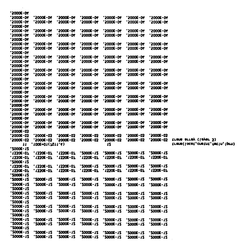
144 13-5

145 13-6

146 For part b, the SSOR package shown below is invoked by setting IUNIT (21) to some finite value and shutting off the SIP package by setting IUNIT (19) to O. MODEL OUTPUT For part a, a sensitivity analysis on the SIP seed and acceleration parameter was conducted. The results are shown in Table In part b, a sensitivity analysis on the SSOR acceleration parameter was conducted. The results are shown in Table Table Sensitivity analysis on SIP seed and acceleration parameter Maximum head change after x iterations Mass balance Total SEED ACCL % error iterations * * * * * * *model calculated seed 13-7

147 Table Sensitivity analysis on SSOR acceleration parameter Maximum head change after x iterations ACCL Mass balance % error Total iterations DISCUSSION OF RESULTS This problem exhibits a large variation in hydraulic conductivities both horizontally and vertically. Consequently, it is difficult to solve numerically. In part & the initial run with model calculated SIP seed and acceleration parameter of 1.0 does not converge in 50 iterations. A trial-and-errror process of optimizing the seed is attempted. By trying order of magnitude variations in the seed, a convergent solution is discovered fairly quickly. The iteration history for seeds of and is shown in Figure Notice that decreasing the seed induces an oscillation in early time, but makes the solution convergence A second alternative of keeping the model calculated seed, while varying the acceleration parameter was also attempted.the results of this scheme were less promising; convergence was not achieved although an acceptable mass balance was attained. In part b the SSOR solution technique was used. A trial-and-error process was again used to optimize the acceleration parameter (Table 13.2). A few trials were required to discover that a convergent solution could be attained between 1.65 and 1.8. The iteration history for acceleration parameters of 1.0, 1.85 and 1.72 is shown in Figure Notice that the high acceleration factor induces oscillation whereas the low acceleration factor causes an asymptotic approach. The SSOR solution technique works fairly well for this problem because most of the heterogeneity is in the vertical. Because SSOR makes a direct solution to slices in the vertical, the heterogeneity is primarily solved for by direct methods. 13-8

148

149 13-10

150 PROBLEM 14 Head-Dependent Boundary Conditions INTRODUCTION The RIVER, DRAIN, GENERAL HEAD, and EVAPOTRANSPIRATION packages of MODFLOW are all head-dependent flux or third type boundary conditions. Although their names imply specific types of sources or sinks, these packages are mathematically very similar and can be used for a variety of hydrologic conditions other than those their names suggest. This exercise illustrates the similarity of the packages, compares results of each to one another as a verification, and gives insight to the utility of parameters used in the packages. PROBLEM STATEMENT AND DATA In order to evaluate these boundary conditions, a single layer, 7 node by 7 node unconfined aquifer is modeled in parts a-d. All cells in the domain are active and a well pumps in the upper left-hand comer (node 1,1). A head-dependent flux boundary condition runs along column 4 for the entire length of the system. The boundary will be treated in five different ways in this exercise. Details on the model specific to all configurations are given in Table Part a) Model the third type boundary condition as a river running down the center of column 4. The river has the following characteristics Elevation Width Riverbed hydraulic conductivity Riverbed thickness River bottom elevation = 0.0 ft = 20 ft = 0.1 ft/d = lft = -2.0 ft Run the model for the 1 year simulation period described in Table Note hydraulic head and boundary discharge at row 1, column 4 for each time step. You will need to invoke the cell-by-cell print flag in both the river package and the output control package. Part b) Model the third type boundary condition as a general head boundary running down the center of column 4. The boundary has the following characteristics: Elevation = 0.0 ft Conductance = 200 ft 2 /d Run the model and note the results as you did in part a. 14-1

151 Table Aquifer parameters and discretization data for Problem 14 Initial head Hydraulic conductivity Aquifer base Storage coefficient Grid spacing (uniform) Pumping rate Stress period length Time steps Time step multiplier SIP iteration parameters Maximum number of iterations Acceleration parameter Closure criterion 10.0 ft 10 ft/d -50 ft ft 2500 ft 3 /d 365 days Part c) Model the third type boundary condition as a drain running down the center of column 4. The drain has the following characteristics: Elevation = 0.0 ft Conductance = 200 ft 2 /d Run the model and note the results as you did in parts a and b. Part d) Model the third type boundary condition as a line of ET nodes running down column 4. These nodes will have the following characteristics: Maximum ET rate Extinction depth ET surface elevation = 0.2 ft/d = 10 ft = 10 ft Run the model and note the results as you did in parts a-c. You will need to store the cell-by-cell ET rates for each time step and then run POSTMOD to put into an ASCII form. Part e) Model the system described above using a two-layer model. The top layer will be the same as in parts ad, except a third type boundary will not be explicitly included. Instead, the bottom layer will represent the third type boundary condition. The bottom layer will be inactive except along column 4, which will be constant head of 0.0 ft. The bottom layer will be confined and have a transmissivity of 100 ft 2 /d. Calculate a VCONT between layers 1 and 2 to give a conductance of 200 ft 2 /d. Run the model and note results as you did in parts a-d. 14-2

152 . MODEL INPUT The following is a listing of the input data sets for part a. 14-3

153 14-4

154 In part b, the RIVER package is substituted with the following GENERAL HEAD package. The flag in the IUNIT array is changed from using the RIVER package to using the GENERAL HEAD package. In part c, the RIVER package is substituted with the following DRAIN package. The flag in the IUNIT array is changed from using the RIVER package to using the DRAIN package. In part d, the RIVER package is substituted with the following ET package. The flag in the IUNIT may is changed from using the RIVER package to using the ET package. 14-5

155 In part e, a two-layer model is constructed. The following BASIC and BCF files are used in conjunction with the previously shown WELL, SIP and OUTPUT CONTROL packages. 14-6

156 MODEL RESULT Table 14.2 shows hydraulic head versus time at node (1,4) for each of the five parts to this problem. Table 14.3 shows discharge versus time at node (1,4). Hydraulic head versus flow is plotted in Figure Table Hydraulic head at node (1,4) for each of the five methods of representing the third type boundary condition Hydraulic Head (ft) Ellapsed Constant Time River GHB Drain E-T head Time Step (days) (part a) (part b) (part c) (part d) (part e)

157 Table Discharge for each of the five methods of representing the third type boundary condition Discharge (ft 3 /d) Elapsed Constant Time River GHB Drain E-T head Time Step (days) (part a) (part b (part c) (part d) (part e)

158 . Figure Hydraulic head (ft) versus flow rate (ft 3 /d) for each of the five methods of representing the third type boundary condition. DISCUSSION OF RESULTS The head-dependent boundary conditions in MODFLOW are all very similar. They allow leakage into or out of the system depending upon the difference in head between the aquifer and some constant head external to the system. The amount of leakage is controlled by a conductance term, which establishes the degree of hydraulic connection between the aquifer and the external source/sink. This exercise demonstrates the equivalency of the boundaries and highlights some of the differences. 14-9

159 The general head boundary is, as the name implies. a general leakage boundary. Flux is directly proportional to head difference for the entire range of saturated conditions. The drain is essentially a one-way general head boundary. Flow can only be out of the aquifer. Evapotranspiration is posed in terms of rates, but it is equivalent to a drain with an upper limit on flux out of the aquifer. Flow cuts off at a certain depth and can only reach a certain upper threshold. Finally, the river is a general-head boundary with an upper threshold of flux into the aquifer. Flow can be into or out of the aquifer, but it can only inflow to an upper limit. The head-dependent flux boundaries can be used for other hydrologic conditions than their names suggest. Table 14.4 shows some other uses for these boundaries. The head-dependent flux boundaries are similar in behavior to a constant-head boundary in an adjacent aquifer. In part e, a VCONT parameter of 200 ft 2 /d/( 100 ft) 2 = O.O2/d was equivalent to a conductance and therefore gave similar answers as the general head boundary. The excellent comparison of the head-dependent flux boundaries to one another provides assurance that they are all implemented in the same fashion. The additional comparison to the two-layer model with adjacent constant head nodes provides a further check that they are implemented correctly in the model. Table Other uses for the head-dependent flux boundary conditions in MODFLOW General Head Boundary Drain River Evapotranspiration Rivers Intermittent streams Adjacent aquifers Drains with maximum flow limitation Exterior model Springs Wetlands boundaries Adjacent aquifers Ditches 14-10

160 PROBLEM 15 Drains INTRODUCTION The drain package of MODFLOW is a third-type or head-dependent flux boundary condition. This exercise demonstrates the utility of the package, provides guidance on computing the conductance term, and compares this boundary to a more detailed characterization of the drain. PROBLEM STATEMENT AND DATA This problem is a simple, one-dimensional flow system which is intersected by a drain. As shown in Figure 15.1, the system is a 120 ft wide strip of a confined aquifer, 1200 ft long with a potentiometric surface which slopes linearly from 10 ft at one end to O ft at the other. The potentiometric surface is established by constant head cells at each end of the model domain. A drain with an effective width of 4.44 ft is placed midway between the two constant head nodes and covers the entire 120 ft strip. The head in the drain is 2.0 ft. A range of conductance values for the drain will be tested and compared to a detailed characterization of the drain as a specified-head condition. The aquifer is isotropic with transmissivity of 100 ft 2 /d. Part a) Set up a coarse-gridded model consisting of 1 layer, 1 row, and 11 columns of 120 ft length. Constant heads of 10 and O ft are placed at columns 1 and 11, respectively. Compute the drain conductance as: (15.1) where: C is conductance, L 2 /T L is length of drain, L (120 ft) W is width of drain, L (4.44 ft) K is hydraulic conductivity of material surrounding drain, L/T (varies) M is thickness of material surrounding drain, L (1 ft). Make several steady-state runs of the model, varying K from ft/d to 100 ft/d. Note hydraulic head in the block containing the drain and the drain flux rate for each K. Part b) Set up a fine-gridded model consisting of the column spacing shown in Table layers, 9 rows, and 60 columns. Use Row spacing is uniform at ft.

161 Layer spacing is 1 ft, 1 ft, 2 ft, 3 ft, 5 ft, and 8 ft, from top to bottom. Constant heads are placed in all layers in columns 1 and 60 at values of 10 ft and O ft, respectively. Two specified-head cells per row (in columns 30 and 31) are used to model the drain. These are set at a head of 2.0 and a hydraulic conductivity of 1000 ft/d to approximate a gravel. A 1 ft-thick-filter layer surrounds the drain on its side and base as shown in Figure Note that the specified-head cells are only in layer 1 while the filter is in layer 1 and 2. Run the model and obtain a hydraulic conductivity for the falter layer which gives an equivalent flux as the 0.1 ft/d hydraulic conductivity used in part a. 15-2

162

163 Table Grid spacing used in the fine-gridded model (Part b) column Width (ft) Column No. No. Width (ft)

164 MODEL INPUT The data set for part a with a K of 0.1 ft/d is shown below. 15-5

165 The data set for part b with a K of 0.1 ft/d is shown below.

166 15-7

167

168 15-9

169 15-10

170

171 15-12

172 15-13

173 15-14

174 15-15

175 15-16

176 15-17

177 15-18

178 MODEL OUTPUT Hydraulic head at the drain node and drain flux is shown for part a in Table Table Hydraulic head at the drain node (column 6) and drain flux for variations in drain conductance (coarse model) Hydraulic head Drain Flux (ft) (ft 3 /d) K = K = K = K = K = K = K=O K=O K = K = K = K = K = K=1OO Constant head 2.00 Constant head DISCUSSION OF RESULTS This problem compares two methods of representing a drain. The first method, using the MODFLOW DRAIN package, represents the drain as an external constant head which is separated from the aquifer by a conductance term. Leakage from the aquifer is due to the head difference between the aquifer and the external drain elevation and is controlled by the user-specified conductance term. Conductance is composed of a number of resistance or head loss producing factors including: hydraulic conductivities in the vicinity of the drain, thickness of material surrounding the drain, size of drain, and drain penetration into the aquifer. Conductance is usually somewhat difficult to quantify because it is a combination of so many factors. Equation 15.1 simplifies the conductance term by establishing a drain size (width x length) and-assuming that the resistance to flow into the drain is controlled by a falter around the drain. It is further assumed that the properties of the filter can be quantified. Regardless of quantification problems, the hydraulic conductivity becomes the variable factor in equation The sensitivity analysis for this problem (Table 15.2) shows that a hydraulic conductivity value of ft/d effectively shuts off discharge whereas a value of 10 ft/d causes a direct connection between the drain and aquifer. The configuration of the fine-gridded model attempts to represent the drain as a set of distinct, quantifiable hydraulic conductivity zones in the aquifer. The drain itself is conceptualized as a gravel zone 2.44 ft wide and 1 ft deep. A wetted perimeter of 4.44 ft is therefore modeled. The gravel is surrounded by a 1 ft-thick layer of porous material. The 15-19

179 hydraulic conductivity of this material was varied in part b of this exercise to match a drain discharge equivalent to the case where K was equal to 0.1 ft/d in the coarse-gridded drain model. A six-layer aquifer is modeled in part b to further characterize the vertical gradients near the drain. The hydraulic conductivity which best matches the ft 3 /d discharge from the coarse model is also 0.1 ft/d. The drain flux for this case is ft 3 /d. Note that the six-layer model has difficulty in converging due to the large variations in hydraulic conductivity from block to block. It is interesting how similar the fluxes generated by these two methods of representing the drain are. Although some of this can be attributed to the linearity and simplicity of the system as well as the thinness of the aquifer, it is apparent that the drain package is a viable means of characterizing drains. The DRAIN package can be used provided that hydraulic conductivity in the drain vicinity can be calculated. Note that the drain behaves as a constant head if the material in the vicinity of the drain is of greater conductivity than the aquifer. In many instances, the conductance is a calibrated parameter that is determined as a part of the modeling exercise

180 PROBLEM 16 Evapotranspiration INTRODUCTION Evapotranspiration is a component of the water budget which is often subtracted from an overall precipitation recharge rate prior to inclusion in the groundwater model. This may be physically appropriate, such as when the water table is sufficiently beneath the subsurface to minimize the effect of evapotranspiration. In other instances, it is not implicitly included due to data limitations. This problem illustrates the utility of the evapotranspiration module and shows how excluding it from an analysis can affect the calibration and predictive capability of the model. The problem also gives an example of how a well may capture water otherwise lost to evapotranspiration. PROBLEM STATEMENT AND DATA The problem domain is a coastal environment covering a regional area of 90 square miles. For the purposes of this analysis, the limestone aquifer extends approximately 8 miles inland and ends abruptly. Groundwater flow lines define the northern and southern extent of the model domain and form no-flow boundaries in those areas. There is some topographic relief in the area, with land surface elevation changing from O ft at the coast to 18 ft in the southwest comer of the domain. A uniformly spaced 20 row by 18 column, finite-difference grid with 2640 ft spacing is used. Boundaries and topographic elevations are simplified as shown in Figure The aquifer is unconfined with base of -200 ft and hydraulic conductivity of 1340 ft/d. Part a) Run the model in a steady-state mode with the EVAPOTRANSPIRATION option and parameters given below: Maximum ET rate = 50 in/yr ET extinction depth =8ft ET surface = land surface may from Figure 16.1 Recharge = 25 in/yr Closure criterion = 0.01 ft Save the output hydraulic heads for later use as an initial condition. Do this using the Hdsv parameter in the Output Control package. Plot the potentiometric surface. Part b) Part c) Subtract the total evapotranspiration rate component in the mass balance of part a from the recharge rate used in part a. Use this as a net uniformly distributed recharge rate, eliminating the EVAPOTRANSPIRATION package. Run the model, plot the potentiometric surface and compare to part a. Using the results of part a as an initial condition, run the model with a well pumping at row 4, column 5, at a rate of 535,000 ft 3 /d. Plot the steady-state drawdown. 16-1

181 Part d) Using the results of part a as an initial condition, run the model with a well pumping at row 17, column 5, and a rate of 535,000 ft 3 /d. Plot the steady-state drawdown.. Figure Finite-difference grid, boundary conditions, and simplified topography for Problem

182 MODEL INPUT The following is a listing of the data set used for part a. 16-3

183 16-4

184 In part b, the evapotranspiration package is turned off by setting IUNIT(5) to O in the BASIC package. The recharge rate (RECH) is changed to ft/d in the RECHARGE package. The following is a partial listing of the part c data set. Note that the initial heads (SHEAD) are the unstressed steady-state results from part a and are read from an external binary file (unit 32) in the BASIC package. A negative unit number directs the model to read an unformatted file. The other packages, BCF, ET, RECHARGE, SIP, and OUTPUT CONTROL are identical to part& and are not shown here. The data set for part d is identical to part c, except the row location for the well (WELL Package) is changed to

185 MODEL OUTPUT ) Figures 16.2 and 16.3 are the potentiometric surface for part a and b, respectively. Figures 16.4 and 16.5 are drawdown plots for parts c and d, respectively. Figure Potentiometric surface (ft) for Problem 16, Part& 16-6

186 Figure Potentiometric surface (ft) for Problem 16, Part b (net recharge). 16-7

187 Figure Drawdown(ft) map for Problem 16, Part c 16-8

188 Figure Drawdown (ft) map for Problem 16, Part d.

189 DISCUSSION OF RESULTS The steady-state results for this problem indicate that the system is dominated by evapotranspiration. The only source is precipitation recharge and 79 percent of this is discharged by evapotranspiration. The remainder (21 percent) discharges to the sea. There is quite a variation in net recharge areally across the system, as shown in Figure Basically, the lower left corner of the model area is a recharge area because land surface elevation is much greater than the water-table elevation. Toward the northeast recharge becomes progressively less until it reaches O where the water table is 4 ft below land surface. This occurs when North and east of this line is all net discharge where ET is greater than 25 in/yr. Notice that the water-table elevation is a subdued representation of the topography. In part b, only the net recharge rate ( ft/d) is applied evenly across the region. As expected from Figure 16.6, this approach is entirely inappropriate because variations in recharge and discharge areas are ignored. 0vera1l heads are much lower than in part a and water levels tend to follow the coastal boundary. In part c, a pumping well is placed in the northwest comer of the model, and the model is run to steady state. A cone of depression develops around the well, with the 0.2 ft contour extending less than half the north-south distance of the model. The maximum drawdown at the well node is 1.19 ft. In part d, a well is placed in the southwest comer of the model. This well pumps at the same rate as the part c well, is in the same column as in part c, and is an equivalent distance from the southern boundary as the part c well was from the northern boundary. Intuitively, the drawdowns in parts c and d should be very similar. Comparison of the results of these two simulations show significant differences, however. The 0.2 ft contour of part d extends greater than half the north-south distance, and the maximum drawdown at the well is 1.57 ft. The reason for the discrepancy is due to the recharge-discharge relationship in the aquifer. In part c (Figure 16.4), the well is located in an area where the water table is close to land surface and evapotranspiration is occurring. When the well is turned on, less discharge occurs as evapotranspiration because the water table is now drawn down. Although the well is a new discharge from the system, the previous discharge from evapotranspiration is reduced. Therefore, the system does not see the full impact of the discharging well. In part d, however, the well is placed in an area where evapotranspiration is not significantly. The well responds with greater drawdown (Figure 16.5) because discharge from evapotranspiration is not significantly reduced. The system in this case sees the full impact of the well

190 Figure Net recharge rates (in/yr) for the steady-state, non-pumping scenario (Part a) 16-11

191 An error exists with using the non-stressed conceptual model as a base for the stressed simulations. Recall that the northern and southern boundaries were no-flow because they were flow lines. When the aquifer is stressed, this approximation is invalidated. For the purposes of this analysis, this error does not change the conclusions previously stated, however it does highlight the fact that the modelers should always be aware of the assumptions inherent to the original model before proceeding to predictive simulations. This exercise highlights the importance of including evapotranspiration in simulations where it is an important component of the water budget and causes natural variation in recharge and discharge areas. Attempting to calibrate a groundwater model with a uniform net areal recharge rate, as is often done, would be inappropriate in this situation. This exercise also illustrates an interesting consideration for well siting. As a check of the MODFLOW results, the hydraulic heads for part a were compared to a similar simulation using the FTWORK (Faust et al., 1989) code. As shown in Table 16.1, the results of the codes are nearly identical. Table Comparison of hydraulic heads (ft) along row 10 for MODFLOW and FTWORK Column MODFLOW FTWORK

192

193 . PROBLEM 17 Wells INTRODUCTION The WELL package of MODFLOW allows the user to specify withdrawal or injection from the modeled area. Wells are assumed to be placed at the center of grid blocks and to fully penetrate the layer for which they are specified. This problem examines situations of partially penetrating wells and multiple aquifer wells. A commonly used rule of thumb is assessed numerically. PROBLEM STATEMENT AND DATA The model domain is essentially the same as that used for the finely-gridded quadrant of the Theis problem (problem It). Instead of the fully penetrating well assumed for problem 1, a partially penetrating well will be analyzed as a part of this problem. In addition, a stratified aquifer with a well fully penetrating 2 layers of varying transmissivity will be assessed. A second layer will therefoxe be required to model these features. Table 17.1 is a listing the physical parameters and discretization data used in the model. Part a) Part b) Part c Part d) Re-run the single layer model used in problem lc for comparison purposes. A well which penetrates only the upper 50% of the model domain is required. Because all wells in MODFLOW & assumed to fully penetrate a model layer, the system will be split into two layers of equal thickness and the well specified for the upper layer. Set up the two layer model. Apportion transmissivity and storage coefficient evenly between the two layers. Assume the entire aquifer thickness is 20 m (10 m per layer) and calculate a VCONT based on an isotropic hydraulic conductivity. Run the model and compare the distance-drawdown relationship at time = s to the distance drawdown relationship at the same time for the fully penetrating case. Assume the thickness of the aquifer is 40 m (20 m per layer) with the same transmissivities and storage coefficients as part b. VCONT is therefore the only parameter which must be recalculated and input to the model. Run and compare distance-drawdown at time = s to parts a and b. Assume that the aquifer system is stratified as 2 layers. The top layer is 10 m in thickness with a transmissivity of m 2 /s and the bottom layer is 30 m thick with a transmissivity of m 2 /s. Storage coefficient is the same as in part a and is distributed based on thickness (equivalent specific storages are used). Note that the net storage coefficient and transmissivity are consistent for parts a-d. Recompute VCONT and input to the model. A fully penetrating well will be used in this application. Because of differences in thickness and hydraulic conductivity of the units, discharges from each layer must be scaled in some fashion. A common method is to use a weighted average: 17-1

194 I (17.1) where: Q N is the well discharge from layer N Q T is the total well discharge T N is the transmissivity of layer N T T is the total transmissivity. Using the same discharge as in parts a-c, apportion flux to the wells. Run the model and compare the distance drawdown relationships at time = s for the two aquifers and to the one-layer simulation. 17-2

195 Table Parameters and discretization used in Problem 17 Initial head Transmissivity Storage coefficient Pumping rate Final time Number of time steps Time step expansion factor SIP iteration parameters Closure criterion Maximum number of iterations Number of rows, columns Number of layers Grid spacing (m): Row number, i (=Column number, j) m m 2 /s x 10-3 m 3 /s (1 x 10-3 m 3 /s for quandrant) s DELC (i) (=DELR(j))

196 MODEL INPUT The data set for part b is shown below. 17-4

197 17-5

198 The part a data set was described in problem 1. In part c, the part b data set is modified - by changing VCONT to E-5/s. In part d the following parameters are used: MODEL OUTPUT T 1 = m 2 /s S 1 = E-4 Q 1 = E-4 m 3 /s T 2 = m 2 /s S 2 = E-4 Q 2 = E-4 m 3 /s VCONT = E-7/s Drawdown versus distance at time = s is tabulated for parts a-din Table These results are plotted in Figures 17.1 and Table Drawdown versus distance at s for the fully penetrating, partially penetrating, and stratified aquifer simulations Drawdown (m) 20 m aquifer 40 m aquifer distance fully partially penetrating partially penetrating Stratified (m) penetrating pumped unpumped pumped unpumped top bottom

199 . Figure Drawdown versus distance for the fully penetrating well case and the partially penetrating well case in the 20 m thick aquifer at time = s. 17-7

200 Drawdown versus distance for the fully penetrating well case and the partially penetrating well case in the 40 m thick aquifer at time = s. 17-8

201 DISCUSSION OF RESULTS This problem illustrates a method of modeling partially penetrating wells. A separate layer is used over the uncased part of the well while the rest of the aquifer is modeled with another layer. In many situations it may not be necessary to incorporate this level of complexity. This was shown in parts b and c, which support the rule of thumb that partial penetration effects vanish at a distance of 0.5 to 2 times the aquifer thickness. For part b, the twenty m thick aquifer, partial penetration effects are minimal at 20m while for part c, the forty m thick aquifer, the effects are minimal at 40m from the well. A multiaquifer well is modeled in part d. Two wells are actually required because MODFLOW assumes one well per layer. Well discharge was apportioned based on a weighted average of the transmissivities. This method results in the same drawdown in the well nodes for the two aquifers, as well as in the most of the aquifers. The weighted average methodology is an intuitive approach which is commonly used. It does not account for some of the complexity inherent in natural systems. Bennett et al., (1982) and McDonald (1984) describe the dynamics of multiaquifer wells and how they may be incorporated in numerical models. 17-9

202

203 PROBLEM 18 Cross-Sectional Simulations INTRODUCTION When conceptualizing flow in a three-dimensional system, it is often useful to simplify the system to a two-dimensional cross-section. In other instances, such as in modeling flow beneath a dam, the entire analysis may lend itself to a cross-sectional representation This exercise shows how to set up a cross-section, illustrates a method of modeling layers of nonuniform thickness and extent, and discusses advantages of certain solution techniques. PROBLEM STATEMENT AND DATA The area to be modeled is near a major river system. A two-dimensional vertical crosssection is useful to conceptualize the flow system, determine reasonable ranges of aquifer parameters, assess model boundaries, and to determine the most influential parameters in the system. Specifically for this problem, the model was used to assess whether aquifer thinning and facies changes could account for a steep hydraulic gradient in that area. The two-dimensional model domain is shown in Figure Most apparent from this - illustration is the highly variable layer thicknesses and pinchouts of certain layers. Partly due to the pinchouts and variable thicknesses, some of the layers have a pronounced dip. associated with them. The model domain is six layers and 27 columns. Because it is a vertical section, a single row is used. The top layer is unconfined, all others are convertible. To avoid calculating unique transmissivities manually for each block a fully convertible option (LAYCON=3) is used such that both aquifer tops and bottoms are read in. A groundwater divide is located on the left side of the model domain. It is implicitly modeled as a no-flow boundary. A specified head boundary condition is used in layer 6 that allows leakage into and out of the overlying system. The river is assumed to penetrate layers 1, 2 and 3 and is modeled as specified head. A divide is assumed beneath the river such that all flow discharges up into the river. The remainder of the right boundary is therefore also assumed implicitly to be noflow. The upper boundary is the water table and receives recharge of in/yr. Because some layers may be desaturated, recharge is assumed to be to the highest active layer. The layer pinchouts are handled by specifying a minimal thickness of 0.5 ft in the area where the bed is absent and assigning a hydraulic conductivity typical of an areally adjacent layer. Therefore, layer 5 has a hydraulic conductivity of 2.8 x 10-5 ft/d for columns 1 through 9 and 28 ft/d for columns 10 through 27. Vertical leakance terms are computed from these hydraulic conductivities and layer thicknesses. Order of magnitude values of hydraulic conductivity are used, with a horizontal to vertical anisotropy of 10 to 1. Hydraulic conductivities are shown below. 18-1

204 Surficial Deposits, A = 0.28 ft/d Clay aquitard, B = ft/d Gravel aquifer, "C" = 28 ft/d Sand aquifer, D = 0.28 ft/d Dense clay aquitard, E = ft/d Leaky clay aquitard, "F" = ft/d Bottom elevations of each layer are given in Table Note that the top elevations for the underlying layer are identical to the bottom elevation for the overlying layer. Initial conditions for the model are 290 ft in the river nodes and 500 ft elsewhere in layers 1 through 5. Hydraulic heads in layer 6 are given in Table 18.2 Horizontal grid spacing is uniform at 1050 ft. For purposes of computing VCONT s for layer 1, the assumed saturated thickness of layer 1 is given in Table Figure Layering and zonation used in the cross-sectional model. 18-2

205 Part a) Part b) Set up and run the model in a steady-state mode. Use the SIP solution technique with an acceleration parameter of 1.0, 5 iteration parameters, closure criterion of 0.01, a maximum of 50 iterations and model calculated seed. Note the number of iterations required for convergence and the iteration history. In case of non-convergence, adjust the SIP seed to obtain a solution. Run the model using the SSOR solution technique with acceleration parameter 1.0. Note the number of iterations required for convergence and the iteration history. 18-3

206 Table bottom and top elevation (ft) in cross-sectional model Layer 1 Layer 2 Layer 3 Bottom Bottom Column Bottom Layer 2 Layer 3 No. Layer 4 Top Top Top Layer 4 Bottom Layer 5 Top Layer 5 Bottom Layer 6 Top Layer 6 Bottom

207 Table 18.2 Initial beads in layer

208 Table Assumed saturated thickness (ft) of layer 1 in the cross-sectional model Column Thickness (ft)

209 MODEL INPUT The data sets for part a are shown below

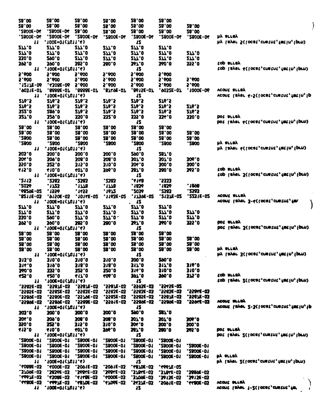
210 18-8

211 18-9

212 In part b, the IUNIT array is modified in the BASIC package to use the SSOR solution technique and the following SSOR package is used. MODEL OUTPUT Hydraulic head arrays for the model are shown in Figure Figure Hydraulic head arrays for the cross-sectional model

213 DISCUSSION OF RESULTS This problem resembles a true field application more than the previous problems. It is, in fact, based on an actual field study. Because this is an actual hydrostratigraphic system, heterogeneity and variable thicknesses are a factor in the analysis. This complicates the model set-up considerably. Preprocessing capabilities become more necessary. The vertical leakance parameter (VCONT) incorporates both hydraulic conductivity and vertical grid spacing. Because VCONT is read as a two- dimensional array, each grid cell can conceivably have a unique thickness. This is somewhat counter to the standard orthogonality of the finite difference method, but can be used provided the grid distortion is not too great. Notice that vertical grid spacing is never used explicitly in MODFLOW; it is always posed in terms of VCONT. A layer must always exist, therefore, a layer cannot simply vanish when a pinchout occurs. Instead, this example models the layer as thinning to a minimal thickness and then taking on the properties of an adjacent layer. In a more general application, properties of layers can be zoned; thinning of layers is not always required. Several statements regarding desaturation appears in the model output NODE (1,1,1) GOES DRY AT ITERATION 9. This indicates that the head in that particular layer has fallen below the specified aquifer base. This may be a physical reality (the case here) or a result of an oscillatory iteration history. Dry nodes in the latter case are a problem because nodes are not allowed to resaturate in MODFLOW. A domino effect may ensue once nodes begin to dry up as a result of oscillatory iteration: the flow system is altered as a result of a dry node, followed by more dry nodes, etc. This type of behavior can be minimized by specifying accelerationparameres and seeds such that an asymptotic solution is approached from a condition of higher head. The SSOR solution technique issuperior to SIP in this particular application. Because the cross-section is taken along a row, the model solves the entire vertical slice by direct means. Some iteration is performed (7) because of non-1inearities due to the upper water table and the dry nodes. Considerably more iterations would have resulted if the cross-section had been oriented along a column. In that case a "slice" would consist of six nodes (1 row x 6 layers) and 27 slices would have been solved. The SIP solution technique requires some adjustment to the seed before it will converge. A convergent solution using 27 iterations was achieved using a seed of Cross-sectional models can often be useful in conceptualization exercises such as this. The user should be careful to align the cross-section along a relatively straight streamtube that has minimal change in width

214

215 PROBLEM 19 Application of a Groundwater Flow Water Supply Problem Model to a INTRODUCTION Groundwater flow models are often used in water resource evaluations to assess the longterm productivity of local or regional aquifers. This exercise presents an example of an - application to a local system and involves calibration to an aquifer test and prediction using best estimates of aquifer properties. Of historical interest, this problem is adapted from one of the first applications of a digital model to a water resource problem (Pinder and Bredehoeft, 1968). The specific objective of their study was to assess whether a glaciofluviai aquifer could provide an adequate water supply for a village in Nova Scotia PROBLEM STATEMENT AND DATA The aquifer is located adjacent to the Musquodoboit River, l/4-mile northwest of the village of Musquodoboit Harbour, as shown in Figure The aquifer is a glaciofluvial deposit consisting of coarse sand, gravel, cobbles, and boulders deposited in a typical U- shaped glacial valley cut into the slates and quartzites of the Meguma group and the granite - intrusive of Devonian age. The contrast in permeability between the granitic and metamorphic rocks and the glaciofluvial valley fill is so great (approximately 10 6 ) that the bedrock is considered as impermeable in the aquifer analysis. The aquifer, which is up to 62 feet thick, is extensively overlain by recent alluvial deposits of sand, silt and clay. The alluvial deposits are less permeable and act as confining beds. A cross-section through the valley is given in Figure A pumping test was conducted to evaluate the aquifer transmissivity and storage coefficient, and to estimate recharge from the river. The test was run for 36 hours using a well discharging at cubic feet per second (432 gallons per minute) and three observation wells (see inset of Figure 19.1 for locations). The test was discontinued when the water level in the pumping well became stable. Initial estimates of aquifer parameters were calculated using the Theis curve and the early segment of the drawdown curves for the observation wells. The results were somewhat variable, ranging from 1.15 ft 2 /s to 1.45 ft 2 /s. A quasi-steady state formula for estimating transmissivity yielded results on the order of 0.3 ft 2 /s. Because of the close proximity of boundaries, the pumping test results are difficult to analyze using usual analytical methods. A listing of the data set for the MODFLOW model is provided on page The aquifer is treated as confined, with transmissivity zones to account for thickness and facies changes. The ratio between zones of transmissivity (1,2, and 4) are given in the data set; absolute values of transmissivity are not given. A map of the transmissivity zones and model boundaries is given in Figure

216 A uniform value of storage coefficient is used in the analysis. The model is used to simulate drawdown, hence an initial head condition of 0.0 ft is used. Recharge is not specified because only drawdown is simulated. A river is simulated using the RIVER package. Its location is shown in Figure Other pertinent data is given in Table Figure Geologic map of the Musquodoboit Harbor region. Inset is the well configuration for the pump test conducted on this aquifer (from Pinder and Bredehoeft, 1968). 19-2

217 Figure Geologic cross-section through the Musquodobit Harbor region(from Pinder and Bredehoeft, 1968). 19-3

218 19-4

219

220 19-6

221

222

223

224 19-10

225 19-11

226 Part a) Part b) Part c) Run the model with the data set provided. Plot the drawdowns at the observation wells and compare to the field data shown in Table 19.2 and Figure Estimate better values of transmissivity and storage coefficient. Do not change location of transmissivity zones. Compare results and continue to adjust T and S until you are satisfied with the results. Make a predictive run for 1000 days at the same pumping rate with the values of T and S that were obtained in Parta. Make some conclusions: How good is your history match? What additional changes might improve it? How important is river leakage? How appropriate is the confined model approximation? How much confidence do you have in your prediction? Is the system at steady-state at 1000 days? What are some weaknesses in this calibration/prediction procedure? What does the modeling indicate regarding the feasibility of using this aquifer as a water supply? 19-12

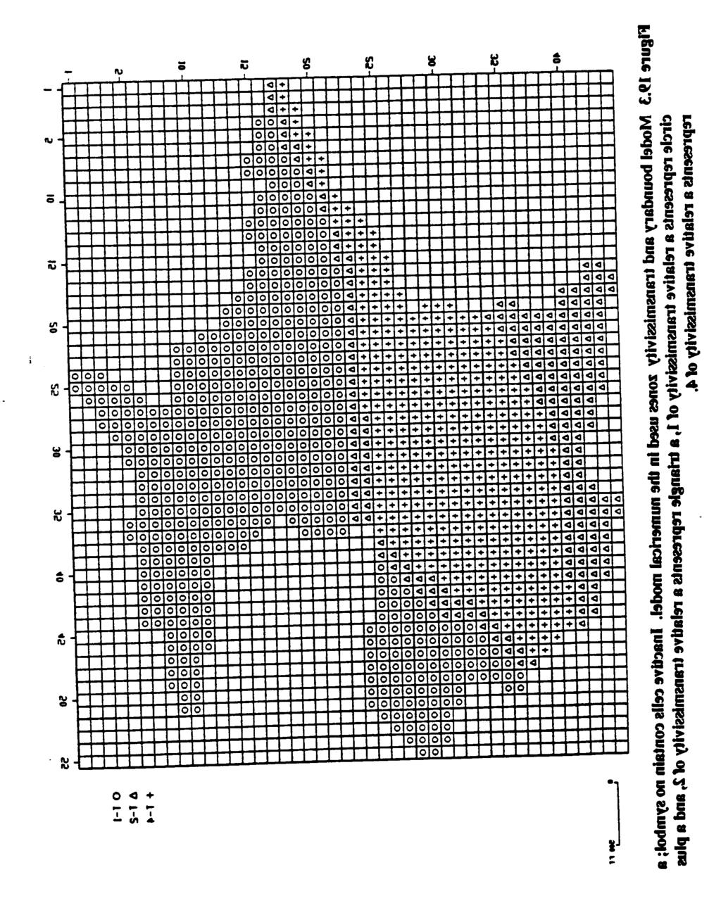
227 19-13

228 . Figure 19.4 Location of the river boundary condition), pumping well, and observation wells use in the numerical model.

229 Table Input data for the water supply problem Grid 44 rows 55 columns, 1 layer Grid Spacing Uniform 100 ft Initial Head 0.0 ft Transmissivity: Non-uniform spatially, 3 zones Storage Coefficient Uniform spatially Closure Criterion Number of time steps 10 The Step Multiplier Length of Simulation 36 hours Production Well Location: row 29, column 32 Pumping Rate: ft 3 /s (432 gpm) River Stage: 0.0 River Conductance: 0.02 ft 2 /s River Bottom Elevation: -l0 ft Table Observed drawdown data from aquifer test Drawdown (ft) Time (min) Well 1 Well 2 Well

230 Figure Drawdown (ft) versus time (min) for the aquifer test conducted at Musquodoboit Harbor. The top line represents observation well 1, the bottom line represents observation well 3. MODEL INPUT Input data sets forthe model were given on page For part a, the transmissivity multiplier that gave the best match for Pinder and Bredehoeft (1968) was while the storage coefficient was In part b, the simulation time (PERLEN) was changed to 1000 days,with 30 time steps (NSTEP), and time step multiplier (TSMULT) of in the BASIC Package. MODEL OUTPUT A comparison of modeled to observed drawdown data for part a is given in Figure Various combinations of transmissivity and storage coefficients yield the drawdowns shown in 19-16

231 Figures 19.7 and 19.8, respectively. The drawdown data for the base case is given in Table A plot of drawdown for part b is given in Figure Figure Comparison of modeled to observed drawdown (ft) data for the base case

232 19-18

233 Figure Comparison of modeled to observed drawdown in wells for the base case and for storage coefficients of 0.1 and

234 Table Modeled drawdown data for the base case. Transmissivities were ft 2 /s, ft 2 /s, and ft 2 /s and storage coefficient was Drawdown (ft) Time (rein) Well 1 Well 2 Well

235 Figure Drawdown (ft) after 1000 days of pumping at ft 3 /s

236 - DISCUSSION OF RESULTS This problem illustrates one type of calibration or history match. In this case aquifer parameters were adjusted in the model to match observed drawdown from a short-term transient event. Within the constraints of the problem statement, adjustments to transmissivity and storage coefficient resulted in the match shown in Figure The match is good in late time, but not in early time. Adjustments to transmissivity change the magnitude of drawdown at a given time (Figure 19.7) while adjustments to storage coefficient changes the shape of the curve before equilibrium is attained (Figure 19.8). The poor match in early time appears to be the result of the storage properties. A decrease in storage coefficient would have the desired effect of increasing drawdown in early time, but would also increase it beyond observed values in later time. To circumvent this dilemma, Pinder and Bredehoeft (1968) introduced a time-dependent storage coefficient to approximate drainage of the aquifer system. The initial value of storage coefficient of was allowed to increase linearly with time to a maximum of 0.06 after 10 minutes of pumping. This is not a standard application and requires either numerous restart simulations or a code modification. Another approximation is to specify a partially convertible aquifer (LAYCON=2) in the BCF package. A closer match (see Figure 19.10) to early time behavior is obtained with a primary storage factor (SF1 ) of 0.003, a secondary storage factor (SF2) of 0.06, and an aquifer top elevation (TOP) of-0.1 ft. Both the time-dependent storage adjustment by Pinder and Bredehoeft and the current magnitude-dependent adjustment are fairly crude approximations to what appears to be a delayed yield effect. The slightly imperfect match to late-time data for the MODFLOW model base case is the result of using Finder and Bredehoeft s (1968) late-time storage coefficient without regard to the early-time factor that they used. As was illustrated in Figure 19.8, a higher constant value of storage coefficient (O. 1 ) results in a better late-time match. River leakage is important because steady-state flow conditions depend on the quantity of water entering the system through the river bed. When the system is at steady state, the pumpage will be balanced by river recharge. The system is close to steady state after 125 days (timestep 24) of pumping as maybe seen from the storage contribution ( ft 3 /s) relative to the river leakage ( ft 3 /s) in the mass balance. The model is mom sensitive to river conductance in late time than in early time. This is shown in Figure The results of all sensitivity simulations for well 1 are given in Table Several potential weaknesses exist in this calibration procedure. The aquifer test provides confidence in parameters close to the pumping well, but less confidence in the characterization distant from the well. The variability in thickness and facies is apparent in the cross-section of Figure 19.2, and yet the representation is fairly simple. Because no wells exist to monitor the effect on the other side of the river, it is difficult to have complete confidence in the characterization of the aquifer/river interaction. This is important because the degree of connection will ultimately govern the productivity of the aquifer. Finally, the need to introduce the delayed-yield effect is not satisfying. Although it is likely that delayed yield is occurring, the representation in the model is very crude. The transient calibration procedure performed here is well suited for a localized aquifer system where the ultimate 19-22

237 some of water is Close to the pumping well. Additional confidence in the calibration could be obtained through a steady-state history match to water levels through the aquifer. The prediction indicates that the aquifer can supply the village with the desired quantity of water with minimal drawdown in the aquifer. The long term drawdown was shown in Figure The results obtained by Pinder and Bredehoeft (1968) and Pinder and Frind (1972) are similar to the current results. This good comparison provides confidence in the applicability of MODFLOW to a field problem. Figure Comparison of modeled drawdown for the drawdown-dependent storage coefficient

238 Figure Comparison of modeled to observed drawdown in well 1 for the base case and for order of magnitude increase and decrease in river conductance

239 Table Drawdown (ft) versus time in observation well 1 for variations in transmissivity, storage coefficient and river leakance Drawdown (ft) Transmissivity Storage Coefficient River Leakance Time (min) Base Case 2X 1/2X

240 -

241 PROBLEM 20 Application of a Groundwater Flow Model to a Hazardous Waste Site INTRODUCTION Despite its inability to assess the mechanisms of contaminant transport a groundwater flow model can provide useful information on various remedial alternatives for hazardous waste sites. Specifically, the flow model can give information on the hydraulic effects, such as flow rates, drawdowns, and flow directions resulting from the remedial alternatives. A contaminant transport model is necessary if data on concentration reduction, mass fluxes, and travel times are desired. This exercise shows how a flow model may be applied to a site, how model input may be adjusted to represent various remedial alternatives, and how model output is interpreted to assess the remediation. This problem is derived from an analysis of conceptual remedial designs at a hazardous waste site (Andersen et al., 1984). The study used an early version of the U.S. Geological Survey groundwater flow model, referred to as USGS2D (Trescott et al ). The model was used to assess the relative effectiveness of a low permeability cap, an upgradient drain, and an upgradient slurry wall. Various combinations of these features were analyzed for their hydraulic merits. Combined with engineering and economic considerations, the results of the groundwater modeling formed the basis of the design which was eventually proposed. PROBLEM STATEMENT AND DATA The waste site is underlain by shallow unconsolidated materials of the Cohansey Formation. The Cohansey consists of an upper sandy zone that varies from O to 30 ft in thickness and a lower silty zone that is 10 to 20 ft thick. A strong contrast in permeability between the two units is apparent from the location of groundwater seeps at the contact between the two units. Underlying the Lower Cohansey is a clay unit of very low permeability. Of most importance at the waste site is the potential for contaminated groundwater migration in the Upper Cohansey and subsequent discharge into surface waters. Further details on the hydrogeology of the site is given in Andersen et al. (1984). A groundwater flow model was calibrated based on observed groundwater levels and discharge measurements from an adjacent stream. The model considers two-dimensional unconfined flow in the Upper Cohansey and uses natural hydrologic features as boundary conditions. A finite-difference grid (Figure 20.1) was designed using smaller spacing (30 ft) near the landfill site where detail was required and larger spacing away from the site near the boundary. Uniform values of hydraulic conductivity (42.5 ft/d), recharge (24 ft/yr), and specific yield (0.28) were used, but a non-uniform aquifer bottom elevation was used. Part a) Use the data set given on page 20-4 to run hydraulic heads on disk for later use in the the steady-state model. Save the transient remedial simulations. 20-1

242 Part b) Part c) Part d) Part e) Simulate the effect of an impermeable clay clap by making adjustments to the recharge array. The extent of the cap is shown in Figure Run for 30.8 yrs with 20 time steps and a time step multiplier of 1.5. Print out mass balances of all time steps and hydraulic heads at time steps 8, 11, 14, 16 and 20. Use a specific yield of Simulate the effect of an impereable clay cap and a low permeability slurry wall. Make adjustments to the hydraulic conductivity array to simulate the wall. The grid cells that contain the wall will have a conductivity of 1x10-6 times that of the aquifer. The extent of the wall is shown in Figure Use the same time stepping and printout specifications as were given in part b. Simulate the effect of an impermeable clay cap, a low permeability slurry wall, and a drain. Use the parameters shown in Table 20.1 in the DRAIN package to simulate the drain. The extent of the drain is shown in Figure Use the same time stepping and printout specifications as were given in part b. Simulate the effect of an impermeable cap and a drain. Use the same time stepping and printout specifications as were given in part b. 20-2

243 - 20-3

244 20-4

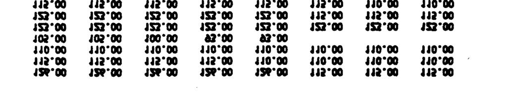
245 20-5

246 I

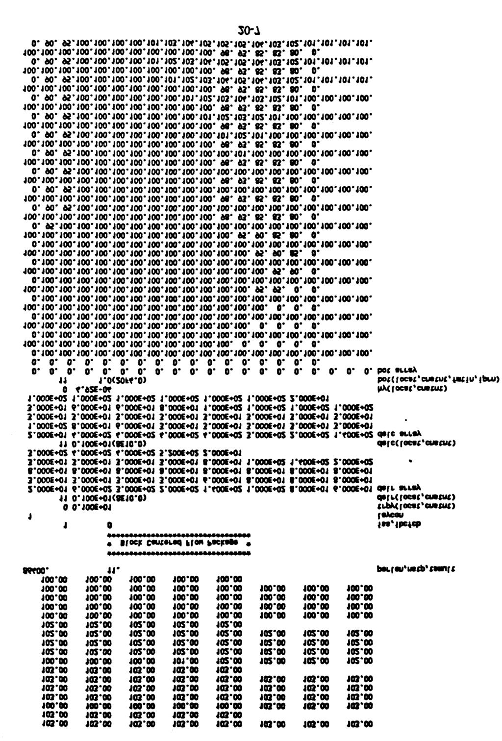
247

248 20-8

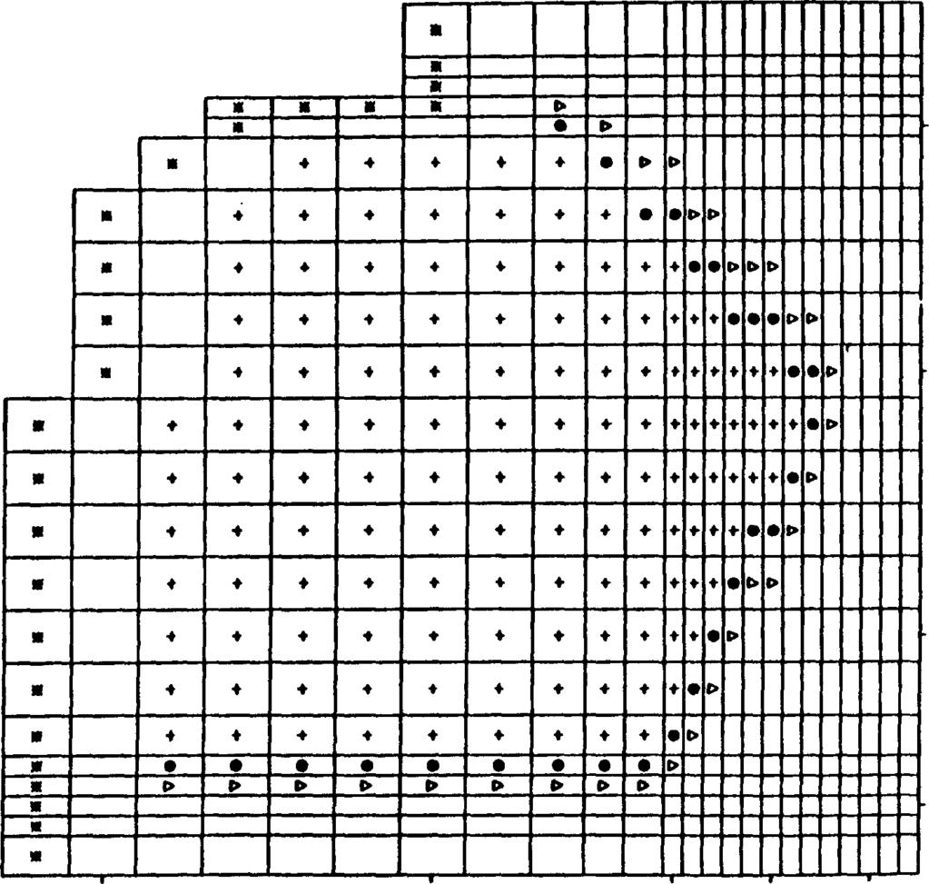
249 .

250 . Table Attributes of the drain used in Part d Conductance Row column Elevation (ft) (ft 2 /s)

251 MODEL INPUT The input data for the steady-state simulation of part a was given in the problem statement. For part b, the input is shown below. Note that the initial conditions are read from the binary file created from the steady-state run

252 20-12

253

254 20-14

255 In part c, the hydraulic conductivity array in the BCF package is changed as shown below to represent the slurry wall. All other parameters are the same as in part b

256

257 20-17

258 In part d, the DRAIN package shown below is added to represent the drain. It is invoked - in the BASIC package in the IUNIT array. All other parameters are the same as in part c. In part e, the BCF package of part b and the DRAIN package of part d are used. The other packages are the same as those used in part d

259 MODEL OUTPUT Hydraulic head contours at 2.69 years in the vicinity of the landfill are shown for four of the five cases in Figures 20.3 ad. Hydraulic heads along column 19 of the model are given in Table 20.2 for the steady state (part a) and the wall and cap scenario (part c). These are compared to the results of the original study, which used the USGS2D code (Trescott et al., 1976). Shown in Table 20.3 are hydraulic heads along column 19 for each remedial alternative. These are plotted in Figure Finally, the drain discharge versus time is shown for each scenario involving a drain in Table Figure 20.3a Hydraulic head (ft) contours in the vicinity of the landfill for the steadystate case (a)

260 I

261 20-21

262 Table 20.2 Comparison of MODFLOW results versus USGS2D results for the steady. state case (Part a) and the wall and cap scenario (Part c) at 6.08 yr. Hydraulic heads (ft) along column 19 of each model are shown

263 Table Hydraulic heads (ft) along column 19 of the model at 2.69 years for each remedial alternative simulation 20-23

264 Figure 20.4 Hydraulic heads (ft) along column 19 of the model at 2.69 years for each remedial alternative simulation

265 Table Drain discharge (ft 3 /s) versus time for the well, cap, and drain scenario (Part d) and the cap and drain scenario (Part e). DISCUSSION OF RESULTS This problem is an example of how a flow model may be applied to assess the effectiveness of various remedial alternatives for sites where contaminant migration is the major concern. The purpose of the original study was to provide input to engineering decisions. Due to data and time constraints many simplifying assumptions were made. The original model configuration has generally been presumed; little, if anything, has been changed to accommodate new technology or new knowledge of the behavior of various remedial alternatives. The cap is simulated simply by limiting recharge. In this case, the cap was assumed to be completely impermeable. A more reasonable approximation is to allow some recharge based on calculations of cap effectiveness. It was further assumed that any precipitation on the cap would be collected before running off without having the opportunity to recharge the aquifer. The effect on the water table of the cap (part b) is to decrease the hydraulic head beneath the cap by one to two feet (see Figures 20.3b and 20.4). Of more importance is the limitation of percolation through the unsaturated zone and subsequent transport of contaminants to the water table. The cap was simulated in all cases because there was no doubt whether it should be used

266 The slurry well is simulated by assigning a hydraulic conductivity of 1x10-6 times that of the aquifer within the grid block representing the well. Assuming a 30 ft wide grid block, this is equivalent to a 2 ft wide wall of hydraulic conductivity 2.83 x 10-6 ft/d or lx10-9 cm/s. This is a very low hydraulic conductivity and essentially represents the wall as impermeable. The purpose of the wall is to reduce flow through the landfill area and to reduce head beneath the cap. As shown in Figure 20.3c, the wall is effective in deflecting water around the landfill. Combined with the drain, the wall allows the drain to collect primarily clean water, thereby limiting treatment costs and reducing the amount of water the drain must transmit. The wall also allows the water table in the landfill area to drop more slowly and causes the amount of solute discharging downgradient to be spread over time. When the wall is used without a drain, some upgradient buildup occurs as the water is diverted around the landfill area. A minor conceptual problem is apparent from figure A buildup of head occurs on the node representing the wall as a result of the recharge on the low permeability wall. Because of the relatively coarse discretization, the entire 30 ft width of the grid block is of low permeability and cannot absorb the recharge. It would probably be most appropriate to assume that water would run off the wall into the more permeable aquifer material. Consequently, recharge could have been redistributed to other nodes in this model or, more accurately distributed in a finer gridded model. The drain is simulated using the DRAIN package of MODFLOW. In the original study, constant head cells were used to represent the drain. This was done primarily because a drain package was not a part of the USGS2D code, but also to assess the maximum amount of flow which could be diverted to the drain. In this application, the DRAIN package was used, but a relatively high conductance based on cell area and aquifer hydraulic conductivity was input. The high conductance value had the net effect of making the drain very similar to a constanthead node. An added benefit of using the DRAIN package was the differentiation in the mass balance between true drain discharge and other constant-head discharge. The drain causes an immediate lowering of the head in the vicinity of the landfill. However, without the Slurry wall, a gradient is established where water flows from the Iandfill area into the drain. Because water comes from both inside and outside the landfill area, flow rates are initially almost twice as high as when a wall is in place (see Table 20.4). The drain without the wall is the most effective of all the alternatives in lowering head in the landfill area Notice in Figure 20.3d that parts of the Upper Cohansey are desaturated after only 2.69 years. A possible weakness of the model configuration of the drain was the need to specify the drain elevation close to the aquifer base. Two-dimensional flow simulated by the model begins to lose some accuracy near the drains where. due to drain placement, flow becomes vertical. Andersen et al., (1984) discuss some of the problems associated with drain placement near the aquifer base and suggest an alternate means of assessing drain flux with the model. Several other scenarios and combinations of remedial measures were simulated in the original study. These included a shorter drain, a less penetrating drain, a smaller cap, a shorter wall, and a drain at greater distance from the wall. The original study also focused on discharge of contaminated groundwater to the seeps downgradient of the landfill. Seep 20-26

267 - discharge was obtained by summing fluxes to pertinent constant-head nodes. Individual nodal discharges may be obtained by invoking the cell-by-cell flow option in the BCF package. The original study also combined the numerica1 results with analytical results as a checking procedure and to verify the validity of simplifying assumptions used in the numerical model. An advective travel time was derived analytically from model results. A more sophisticated method of assessing advective contaminant migration with a flow model is to use a particle tracking module, such as MODPATH (Pollack, 1989)

268

269 REFERENCES Andersen, P.F., C.R. Faust, and J.W. Mercer, Analysis of conceptual designs for remedial measures at Lipari Landfill, New Jersey. Ground Water Vol. 22, no. 2 pp Bear, J., Dynamics of fluids in porous media. American Elsevier, New York. Bennett D., Kontis, A.L. and Larson, S.P., Representation of multiaquifer well effects in three-dimensional ground-water flow simulation, Ground Water v. 20, no. 3, pp Bredehoeft, J. D., and G.F. Pinder, 1970, Digital analysis of areal flow in multiaquifer groundwater systems a three-dimensional model. Water Resources Res., 6, pp Faust, C.R., P.N. Sims, C.P. Spalding, P.F. Andersen, and D.E. Stephenson, FTWORK: a three dimensional groundwater flow and solute transport code. Westinghouse Savannah River Company WSRC-RP Franke, O. L., Reilly, T. E.. and Bennett, G.D., Definition of boundary and initial conditions in the analysis of saturated ground-water flow systems -- An introduction: U.S. Geological Survey Techniques of Water-Resources Investigations, Book 3, Chapter B5. Freeze, R.A. and J. Cherry, Groundwater, Prentice Hall, Englewood Cliffs, NJ 604 pp. GeoTrans, SEFTRAN: A simple and efficient two-dimensional groundwater flow and transport model, Version 2.7. Software documentation. Hantush, M.S., Modification of Theory of Leaky Aquifers, Journal of Geophysical Research, 65 pp McDonald, M.G., Development of a multi-aquifer well option for a modular groundwater flow model. Proceedings of the FOCUS conference on practical applications of groundwater models. NWWA

270 1 Papadopulos, 1. S., Nonsteady flow to a well in an infinite anisotropic aquifer, Symp. Internn. Assoc. Sci. Hydrology, Dubrovnik Pinder, G.F. and J.D. Bredehoeft, Application of the digital computer for aquifer evaluation. Water Resources Research, Vol. 4, pp Pinder, G.F. and E.O. Frind, Application of Galerkins procedure to aquifer analysis. Water Resources Research, Vol. 8, pp Pollack, D.W., Documentation of computer programs to compute and display pathlines using results from the USGS modular three dimensional finite difference groundwater flow model, U.S. Geological Survey Open File Report Prickett, T.A., and C.G. Lonnquist Selected computer techniques for groundwater resource evaluation. Illinois State Water Survey, Bulletin 55, 62 pp. Reilly, T. E., Franke, O. L., and Bennett, G.D., The principle of superposition and its application in ground-water hydraulics: U.S. Geological Survey Techniques of Water- Resources Investigations, Book 3, Chapter B6. Rushton, K.R. and L.M. Tomlinson, Permissible mesh spacing in aquifer problems solved by finite differences, Journal of Hydrology 34: Theis, C.V The relation between the lowering of the piezometric surface and the rate and duration of discharge of a well using groundwater storage. Trans. Amer. Geophys. Union, 2, pp Trescott, P. C., G.F. Pinder, S.P. Larson, Finite-difference model for aquifer simulation in two dimensions with results of numerical experiments: U.S. Geological Survey Techniques of Water-Resources Investigation, Book 7, Chapter Cl, 116 p. van der Heijde, P.K.M. and R.A. Park, Report of findings and discussion of selected groundwater modeling issues, Study conducted under cooperative agreement CR with the U.S. Environmental Protection Agency, R.S. Kerr Environmental Research Laboratory, Ada, OK R-2

271 APPENDIX A Abbreviated Input Instructions These input instructions are intended as a quick reference for the experienced user. Most explanations that are contained in the complete input instructions given in package documentation have been omitted. The format of input fields is given only for those records that contain fields that are not 10 characters wide. Each input item, for which format is not given, is identifed as either a record or an array. For records, the fields contained in the record are named. For arrays, only the array name is given. Input fields which contain codes or flags are described. All other field and array descriptions have been dropped. The real two-dimensional array reader (U2DREL), the integer two-dimensional array reader (U2DINT), and the real one-dimensional array reader (UIDREL) read one may-control record and, optionally, a data array in a format specified on the array-control record. FOR REAL ARRAY READER (U2DREL or UIDREL) Data LOCAT CNSTNT FMTIN IPRN Format 110 F1O.O 5A4 I10 FOR INTEGER ARRAY READER (U2DINT) Data: LOCAT ICONST FMTIN IPRN Format I10 I10 5A4 I10. IPRN is a flag indicating that the array being read should be printed and a code for indicating the format that should be used. It is used only if LOCAT is not equal to zero. The format codes are different for each of the three modules. IPRN is set to zero when the specified value exceeds those defined in the chart below. If IPRN is less than zero, the array will not be printed. 11G I1 9G I2 15F7.1 30I3 15F7.2 25I4 15F7.3 20I5 15F7.4 20F5.O 20F5.1 20F5.2 20F5.3 20F5.4 10G11.4 A-1

272 LOCAT--indicates the location of the data which will be put in the array. If LOCAT <0, unit number for unformatted records. If LOCAT = O, all elements are set equal to CNSTNT or ICONST. If LOCAT >0, unit number for formatted records. ) Basic Package Input Input for the Basic (BAS) Package except for output control is read from unit 1 as specified in the main program. If necessary, the unit number for BAS input can be changed to meet the requirements of a particular computer. Input for the output control option is read from the unit number specified in IUNIT(12). FOR EACH SIMULATION 1. Record: HEADNG(32) 2. Record: HEADNG (continued) 3. Record: NLAY NROW NCOL NPER FOR EACH STRESS PERIOD 9. Data: PERLEN NSTP TSMULT ITMUNI--is the time unit of model data. O - undefined 3- hours 1- seconds 4- days 2- minutes 5- years Consistent length and time units must be used for all model data. The user may choose one length unit and one time unit to be used to specify all input data. IUNIT--is a 24-element table of input units for use by all major options. IAPART --indicates whether array BUFF is separate from array RHS. If IAPART= O, the arrays BUFF and RHS occupy the same space. This option conserves space. This option should be used unless some other package explicitly says otherwise. If IAPART # O, the arrays BUFF and RHS occupy different space. A-2

273 Input to Output Control is read from the unit specified in IUNIT(12). All printer output goes to unit 6 as specified in the main program. If necessary, the unit number for printer output can be changed to meet the requirements of a particular computer. A-3

274 I Block-Centered Flow Package Inut Input for the BCF Package is read from the unit specified in IUNIT(l). All of the arrays (items 6-12) for layer 1 are read fret; then all of the arrays for layer 2, etc. A-4