Feasibility Study of Artificial Aquifer Recharge in the Walla Walla Basin. Presenter: Arístides Petrides

Transcription

1 Feasibility Study of Artificial Aquifer Recharge in the Walla Walla Basin Presenter: Arístides Petrides

2 Overview of Presentation Background Walla Walla River Basin Previous Modeling Effort with IWFM New Model Objectives Model Development Model Calibration Preliminary Results Recharge Basin Analysis Summary

3 The Walla Walla Basin is shared by the states of Oregon and Washington. The model area is 231 km2 (90 mi2) Continental climate: Cold winters, hot summers Precipitation 25 to 38 cm/year Oct-May Elev: 320 m to 228 m Walla Walla Watershed. Pink delineation of new model area, black delineation of previous model area Petrides (2008).

4 Background In 1998 listed as America s 18th Most Endangered River. Irrigation Districts agree to leave 0.7 m3/s (25cfs) in the river. New management practices are required. Evaluating alternatives: Artificial recharge, Lining irrigation canals, Build a surface reservoir.

5 Objectives Assemble what is known about the basin Modeling demands all information known Understand the hydraulics of the system Predict the influence of management Recharge Basins Lining Canals Pumping Shallow Aquifer Develop Selection Methodology for Recharge Basin Location and Size to Enhance Habitat Provide a Tool Suitable to Diverse Applications

6 Previous Model Results

7 Surface Water Representation The total number of stream reaches: 67 Total length of stream segments: 220 km (137 mi) Number of stream nodes:2015 The surface water features in IWFM includes the Walla Walla River, springs and irrigation canals.

8 Lining irrigation canals will cause cessation of flow in springs Springs The groundwater that makes the flow in the springs: Johnson Creek, Dugger Creek and Mud Creek is the water lost through infiltration of the unlined irrigation canals.

9 Previous Model What we learned from the previous modeling effort is: 1. Lining the canals will result in the cessation of flow of springs 2. Artificial aquifer recharge water could maintain aquifer levels to increase flow in the targeted springs 3. Water budget analysis showed that there is the potential for more water to be artificially recharged in the winter months

10 Differences Between the Previous and the Current Model Model area increased from 43km 2 to 231km 2 Decreased node spacing from 400 to 100 m Increased from 400 to 36,500 elements. Number of monitored wells increased from 40 to 90 Number of river reaches increased from 20 to 67 Aquifer recharge projects modeled as lakes in IWFM 3 New version of IWFM

11 Walla Walla Model Summary Model area : 231 km Average node spacing: 100 m Total number of elements: 36,500 Number of aquifers : 2 Stream segments: 67 (220 km) Number of land uses: 20 GIS map of the model area. Blue lines represent the major surface water features represented in the model. Number of artificial aq. recharge: 3

12 Model Building grid size On average, we have a node every 100 m. We have a total of 18,520 nodes for 36,480elements. Model grid showing 4 to 5 elements per parcel of land. The grid is 75% smaller on the A.R. projects

13 Aquifer Recharge in IWFM Aquifer recharge is modeled as a lake in IWFM We are simulating 3 current aquifer recharge projects

14 Models evaluate and organize observation data. What is measured in the field: Water levels in wells 117 obs Flow in rivers, canals and springs 45 gauges Reference evapotranspiration and precip. 3 stations What is estimated: Water and Land use # of water usages Pumping gravels or basalt aquifer 100 Basalt-Wells Aquifer thickness 3 aquifer layers Surface elevation 10m DEM

15 Model Representation of Aquifer System Thickness of aquifer layers: Touchet beds 0 to 6 m Young gravel: 10 to 20 m Old gravel: 23 to 84 m Clay aquitard: 70 m Basalt layers From: Test Site Geology, Hydrogeology and Water Quality (Lindsey 2004)

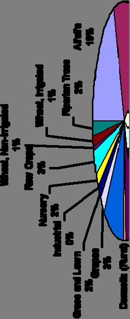
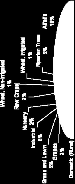
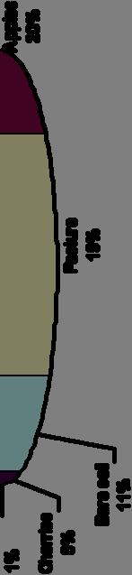
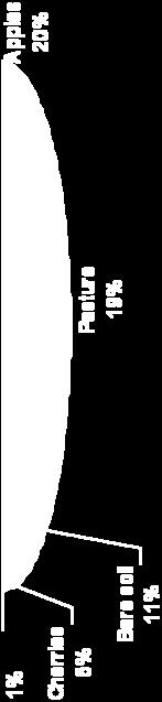
16 Water and Land Use 7 Sub regions 20 water uses (17 crops) Evapotranspiration Pumping estimates 20 land uses 17 diff. crops Et act =(ET o *K c )K s FAO 56 Penman-Monteith

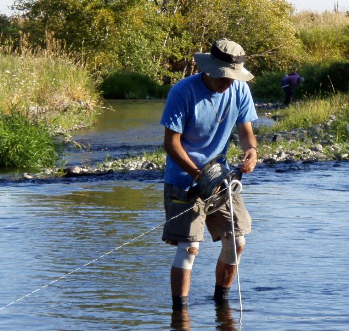
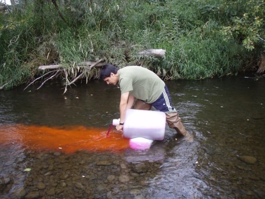
17 Field Work to Estimate Initial Parameters

18 Assessing Sensitivity of Model to Parameters Which parameters are most influential? Conductivity? Soil porosity? Crop coefficient? To assess, we need an overall metric of performance Wells and stream flow have different units of measurement and uncertainty We compute a weight for each observation point so the difference between model and observation are consistent

19 Examples of Sources of Uncertainty Barometric adjustment X,Y location GPS Elevation GPS Non-model local process (pumping) Node location vs well location Instrumentation error Instrumentation setup and maintenance Each has a variance, and the weight is ω=1/σσ 2

20 Monitored Locations QA & QC of gauge database GIS map of the model area. Blue dots represent monitored wells. Green squares represent continuous surface water gauges.

21 Sensitivity Analysis Sensitivities are derivatives of dependent variables with respect to model parameters. Calculated by central or forward differences. In other words: How much does the model output change as the parameters change? dh dp = h( p + Δp) Δp h( p) In order to compare the sensitivities of different parameters, we need to use the same scale. Mary Hill (2007) proposes to use the following statistics dss = dh dp 1/ pω 2 css = NO 1 ( dss 2 / NO) 1/ 2

22 Composite Scale Sensitivities for 27 parameters GW & SW

23 Calibration of Selected Parameters Variable Acronym Starting Value Estimated Value max min Hydraulic conductivity Quaternary Ks Hydraulic conductivity Mio- Pliocene Ks Specific Storage of aquifer 1 EspStor Specific Storage of aquifer 2 EspStor Specific yield aquifer 1 Espyield Specific yield aquifer 2 Espyield Vertical conductivity 1 VertK Vertical conductivity 2 VertK Vertical conductivity soils UZ K vert Agricultural Re-use water Re-use Streams leakage over Touchet K river touchet Streams leakage over quaternary QK rivers

24 Parametrization ( h obs h h )*( ) p2 2 1 p2 h P p1 P = P obs P 2 Suggested Simplification of Gauss-Newton Parameterization

25 Statistical Measurements of Overall Model Fit Sum of Squared Error 200 Obs. SD (GW only) 2.4 * ,969 3 m Nash 0.88 R GIS output map showing the SD at all wells without weights in the model area.

26 Water Budget Analysis

27 Water Budget as Cumulative Flow & Irrigation Source 34% 66% Pumping irrigation Surface water irrigation

28 Transferring a Complex Model to a User Community Technology Transfer Consultation Orientation Guidance practice period Benefits Model Validation Data sharing and transparency Project outreach & community involvement

29 Minimum Flow Necessary in the Walla Walla River HBDIC Recharge Site Legal Diversion Periods November 1st through November 30th Minimum Walla Walla River Flow Q min 65 cfs (m 3 /sec) December 1st through January 31st 95 cfs (m 3 /sec) February 1st through May 15th 150 cfs (m 3 /sec) These minimum instream flows were determined through the OWRD limited testing license process in 2004 in consultation with Oregon Water Resources Department (OWRD), Oregon Department of Fish and Wildlife (ODFW), Oregon Department of Environmental Protection (ODEQ) and the Confederated Tribes of the Umatilla Indian Reservation (CTUIR). Bower (2009). Hudson Bay Recharge Testing Site Report

30 Examples of Potential Recharge Locations Land use availability for aquifer recharge by Rick Henry WWBWC personal communication

31 Evaluation of Recharge Locations: 5 suggested criteria 1. Groundwater flow distance to desired surface water discharge (Ln) 2. Depth to the water table (H) 3. Available area for basin (A) 4. Calculation of maximum recharge rate (Bouwer 1999) H 2 ir Rn = 1 + 2ln 4T R 5. Use of IWFM to test the effects of the proposed AR project Vectors of groundwater show the direction Water table map

32 Example HBDIC 1. Distance to Johnson and Dugger Creek Ln=1,600 m 2. Distance to the water table H= 14 m 3. Available area for recharge A=200 * 50 equivalent radius of 56.5 m 4. Solving H 2 ir Rn = 1 + 2ln 4T R Radial flow theory, Bouwer (1999) 4*30*60*14 1 i = * = 4.1( m / day) ln i = Q A 3 Q = 4.1*10,000 = 41,200( m / day) = 17cfs 5. Scenario C from masters

33 Acknowledgements This project thanks the following organizations for their funds through the Walla Walla Basin Watershed Council Oregon Watershed Enhancement Board Washington Department of Ecology Bonneville Power Administration