Nutrient Loads: Overview of approaches, and the Chesapeake Bay experience. Robert M. Hirsch, Research Hydrologist US Geological Survey

Transcription

1 Nutrient Loads: Overview of approaches, and the Chesapeake Bay experience Robert M. Hirsch, Research Hydrologist US Geological Survey

2 Outline of the presentation 1. Multiple reasons to estimate loads 2. Sampling approaches 3. Calculation approaches 4. A story: The thrill of victory, the agony of defeat 5. The Chesapeake Bay Experience

3 Motivation: Quote From Ralph Keeling The only way to figure out what is happening to our planet is to measure it, and this means tracking changes decade after decade and poring over the records. Keeling, 2008, Recording Earth s vital signs, Science, p

4 Why estimate loads? 1) To understand how a Lake responds to inputs, we need a time-history of inputs. 2) To build early warning systems. 3) Estimate long-term averages to compare watersheds. 4) Assess progress toward watershed goals. 5) Build understanding of the impacts of various management practices.

5 How do we gather the data? 1) Collect a water sample such that it integrates the flux over the whole cross-section. 2) Collect a sample from the water surface. 3) Collect a sample from a fixed point at depth in the cross section. 4) Use sensors at a fixed location in the cross section to measure surrogates.

6 Can these provide unbiased estimates of load? 1) Collect a water sample such that it integrates the flux over the whole cross-section. YES 2) Collect a sample from the water surface. YES if calibrated with whole cross-section. 3) Collect a sample from a fixed point at depth in the cross section. YES if calibrated with whole cross-section. 4) Use sensors at a fixed location in the cross section to measure surrogates. YES if calibrated with whole cross section.

7 When do we gather the data? 1) On a fixed calendar (e.g. weekly or monthly) 2) On a fixed calendar plus high flow events 3) Approximately daily (perhaps increased during events) 4) Sensor measurements at very high frequency

8 5 broad categories of calculation methods They each have multiple variations Their suitability depends on the characteristics of the data set and behavior of the variable Probably all have an appropriate use, but we need to be mindful of their strengths and weaknesses

9 Major distinctions among methods How do we portray E(C) as a function of Q? Do we use data from one year to help predict loads in other years? How do we treat seasonality? How do we estimate the variability? How do we use samples close to the time for which we are making the estimate?

10 Selection of methods needs to be driven by two primary factors What s the nature of the data set? In particular, what s the frequency at which the data are collected (data may be a sample or an instrument reading)? What s the question we are trying to answer?

11 Ratio estimates C Can make it seasonal. Q Excellent from a bias standpoint. Excellent with large data sets. (e.g. 500 per decade) How do they use data beyond the year collected?

12 Regression estimates ln(c) Can make it seasonal and can handle long-term trend. ln(q) Can have bias problems if not careful. Well suited to moderate data sets. (~150 per decade) Curvature and extrapolation issues can be serious.

13 Interpolation methods C Composite method is a hybrid between regression and interpolation. It interpolates regression residuals. time Great if samples are frequent. (>2000 per decade) Terrible with large gaps. If events happen between samples: very poor.

14 Smoothing: WRTDS (or GAM) Concentration Performs well with respect to bias. Best with >200 samples in a decade.

15 Surrogate Regressions ln(c) Sensor might be turbidity, nitrate, specific conductance,? sensor value Multiple sensors can be used simultaneously Well suited to moderate data sets. (~150 per decade) Less prone to extrapolation errors.

16 An aside about evaluating methods We need to look at the data both from the standpoint of concentration and the standpoint of load.

17 2e+05 1e Maumee River at Waterville OH Total Phosphorus in mg/l as P Flux versus Discharge Regress log(flux) on log(q) R 2 = Flux in kg/day Discharge in m 3 s

18 Concentration in mg/l Maumee River at Waterville OH Total Phosphorus in mg/l as P Concentration versus Discharge log(concentration) on log(q) R 2 = Discharge in m 3 s

19

20

21

22 What are my points here Hard to see the lack of fit when estimating log(flux). R 2 is not informative. Easier to see lack of fit when estimating log(concentration). R 2 is meaningful. Best to see lack of fit looking at residuals. Using polynomial fits may cause the tail to wag the dog and bias estimates at the high discharges.

23 One more thought about looking at residuals Never forget to look at real loads. Data set is nitrate from Raccoon River at Des Moines, IA WRTDS Loadest 7

24 Selection of methods needs to be mindful of some common properties of water quality data Relationship to discharge Seasonal variations Typically skewed May be censored ( less than values ) Serial correlation

25 Selection of methods Do the methods consider the actual properties of the data? Have we put them to a test against very rich data sets?

26 Selection of methods: Consideration of purpose of the analysis Assessements of progress can be easily obscured by the random, but persistent, patterns of wet and dry years I call this: The thrill of victory, the agony of defeat

27 7 Potomac River at Washington, DC Total Phosphorus Water Year Annual Flux Estimates 6 5 The thrill of victory Flux in 10 6 kg yr

28 Look at the discharge record 25 Potomac River at Washington, DC Water Year mean daily Four dry years 20 Discharge in 10 3 ft 3 s

29 7 Potomac River at Washington, DC Total Phosphorus Water Year Annual Flux Estimates 6 Flux in 10 6 kg yr The agony of defeat

30 25 Potomac River at Washington, DC Water Year mean daily 20 Discharge in 10 3 ft 3 s It s all about the flow!

31 Some might say, you can get rid of the problem if you just look at concentration rather than flux 0.18 Potomac River at Washington, DC Total Phosphorus Water Year Annual Mean Concentration 0.16 Concentration in mg/l Sorry to say, the problem remains

32 What s my point here? Although the history of loadings can be very useful to ecologists studying the drivers of the receiving water body It is not useful for assessing progress in the watershed. We are smarter than Homer! We can deal with the influence of flow.

33 How might we do this? Develop a statistical model for how the system behaves in response to discharge and season (exogenous variables). And how the system behavior changes over time. Then integrate that over the distribution of discharge (and season) to describe the trend in watershed behavior.

34 We want to describe to the managers: How the system behavior is changing, independent of the particulars of the yearto-year random variation in discharge. One approach is to use the annual values of flow-normalized flux, one of the outputs of WRTDS (Weighted Regressions on Time, Discharge and Season)

35 Chesapeake Bay Experience Slides are from Doug Moyer, USGS, Virginia Water Science Center: coordinator of the Non-tidal network for Chesapeake Bay Program. Data collection by several agencies Load and trend in load results are at

36 Chesapeake Bay Nontidal Monitoring Network Monitoring Stations 117 monitoring stations 30 with records > 30 yrs 87 with records > 10 yrs 30 (green on map) with records < 5 years Drainage areas range from 1 to 27,100 mi 2 Six States, D.C., SRBC, USGS, and EPA $6M Annually - $50K per site USGS responsible for load and trend computation Discharge data available at all sites Sampling by Equal Width Intervals (integrated samples with isokinetic samplers)

37 Data Collection Sampling Goals Collect 20 water-quality samples per year 12 Routine Samples 8 Storm-Impacted Samples (required for load quantification) Water-Quality Measurements Streamflow Field parameters Nitrogen (TN, DN, PN, NOx, NH 4+ ) Phosphorus (TP, DP, PP, SRP) Sediment (SSC, TSS, VSS, FSS)

38 Equal Width Increment EWI

39 Data Collection WBH-96

40 Data Collection DH-95

41 Total Nitrogen per Acre Loads Total nitrogen loads range from 1.19 to 33.4 lbs/ac with an average load of 7.33 lbs/ac 3 Categories of Loads: (1) Low = 6.88 lbs/ac 52 of 81 stations (2) Medium = > 6.88 to of 81 stations (3) High Yields = of 81 stations

42 Total Nitrogen per Acre Loads and Trends: Improving Trends = 44 of 81 (54%) Degrading Trends = 22 of 81 (27%) No Trend = 15 of 81 (19%) Of the 14 stations with the highest per acre loads for Total Nitrogen: 6 have improving trends 3 have degrading trends 4 have no trends 1 has insufficient data for trends Results by major basins

43 Changes in Nitrogen per Acre Loads: Example from the Susquehanna Watershed

44 Changes in Nitrogen per Acre Loads: Trend in load network is the first of its kind Improving Stations Range = to lbs/ac Median = lbs/ac (-10.0%) Degrading Stations Range = 0.04 to 1.21 lbs/ac Median = 0.33 lbs/ac (7.84%) Download figure:

45

46 These results are being used to: explain change enhance models measure progress inform strategies It is built on a 3-decade effort with many partners.

47 Parting thoughts Developing an integrated network has been a large and long-term investment. The Chesapeake Bay Program is now seeing payoffs. Because of the uniform loading-trend results there is now a very active interagency research program on Factors Affecting Trends Already have found at least two areas where the TMDL model and observations don t agree Role of stored phosphorus in soils with conservation tillage Changing trapping efficiency of an old reservoir.

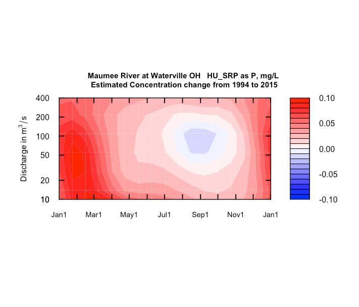
48 Parting thoughts - 2 WRTDS does more than provide a measure of progress It provides tools for improved understanding The EGRET-R software, provides a toolbox for many types of inquiries. WRTDS and more. EGRET = Exploration and Graphics for RivEr Trends A couple of examples:

49

50

51

52 Trend from 1995 to 2005 = +6% per year Trend from 2005 to 2015 = +0.7% per year

53 Two examples where the difference between concentration trends and flux trends proved to be highly informative

54 Concentration in mg/l Choptank River near Greensboro, MD Nitrate Water Year Mean Concentration (dots) & Flow Normalized Concentration (line) Concentration trend +40% Flux in 10 3 kg yr Choptank River near Greensboro, MD Nitrate Water Year Flux Estimates (dots) & Flow Normalized Flux (line) Flux trend +27%

55 trend +2.2%/yr trend +5.4%/yr

56 Parting thoughts - 3 Protocols don t have to be identical, but their functional similarity needs to be demonstrated The Chesapeake Bay network was planned over 20 years ago using the best technology at the time. In my opinion, evolving technology points the way to more use of continuous sensors, coupled with highly-accurate calibration samples on a regular basis over a range of conditions. For loading trends there will need to be explicit consideration of the drift in the relationship of instrument values to actual concentrations.