Hydroponic Treatment Trial

Transcription

1 Hydroponic Treatment Trial A Trial conducted on Hydroponically grown cucumbers to examine long term and short term effects the technology has on living cellular structures. Trial conducted 1998 Location: Helidon, Queensland Australia

2 Abstract The study contained herein, details the observations and effects produced by the Bio-field Technology as applied in a commercial cucumber production facility. The following is a summary of these effects Improved plant health Observed, healthier greener colour and stronger supporting stems. Improved resistance or tolerance to disease While untreated plants wilted away, under the attack from a fungal disease, the treated plants remained greener and appeared healthier. Improved tolerance to weather conditions Where the untreated plants received tip burns during periods of higher temperatures, none of the treated plants showed any signs of weakening. Increased growth rate The increase in growth noticed, was not just from the fact that the treated plants outgrew the untreated, but also from the fact that, the treated plants initially received less water than that required. They still looked fine, but the growth rate was not as high as that of the untreated. This was then corrected, where after, the treated plants quickly caught up and then exceeded the growth of the untreated plants and yet, the treated plants still received less water and nutrients than did the untreated, about 60ml less on average throughout the trial. [Amendment] Subsequent trials revealed that the early growth rate difference was not a result of the water delivery system. Repeat trials also reproduced the same growth rate patterns. The treatment caused a delay in the onset of maturity in the plants which turned out to be very beneficial to the plant and a major biological discovery for us. Increased number of Nodes An increase in the number of nodes from which a fruit would grow was noticed and hence counted. This showed an increase of up to 20% more nodes on the treated plants, at the time of counting, however, considering that the final yields had improved by 40% to 57% per plant; this increase in node count would have varied throughout the trial. Increased Yield and Hence Profit Treated Rows, 2 & 3 represents 23.3% (less than a quarter) of the overall plants in the shadehouse, The remainder 76.7% of the plants were not treated, yet the treated rows produced 30.9% (Close to a third) of the total production in the shade-house. The yield rejection remained mostly the same, regardless of the increase in yield, effectively decreasing the rejection ratio from 41.4% to 31.6%. On average, the treated plants could produce 9.97 Cucumbers per plants, compared to 7.15 cucumbers at best, per plant using current methods. See the Financial Projection Page.

3 Please note that no scientific testing has been done on the plantʼs ability to withstand or tolerate extreme weather conditions or cope better with a disease. The grower has made these observations through experience. Hydroponic Trial Set-up Layout The hydroponics trial was conducted in Helidon, 19 Km East of Toowoomba, Queensland, Australia, at facilities owned by Mr. & Mrs. Grorud. The Trial was commenced on the 6 th of February The shade-house utilized for this trial was a steel-framed construction and was covered with clear plastic over two thirds of the surface. The remaining area was covered with a shade cloth on the lower parts of both sides. A Clear plastic cover could also be rolled down over the shade cloth in extreme weather conditions. The plants grew in 8 rows within the shade house, where each row had been designated a number by the grower as is shown in Figure 1 below. The two trial rows being irrigated with the charged water were in the center of the shadehouse with the control row one row across to the right. The plants in the trial row No. 2 grew in sawdust and the plants in row No. 3 grew in coal ash. The control row designated as row No. 1 grew in sawdust. Each row contained a set number of plants as outlined in Table 1 below. Number of plants in each row Row

4 Plants Table 1, Number of plants in each row Water delivery system The water delivery system already connected to the shade-house was set to pump 80 Liters per minute for a set amount of time, which delivered a controlled quantity of water to the entire shade-house, each time it was watered. Rows 2 & 3 contained 141 Plants of a total of 604 plants, which means that by proportion, rows 2 & 3 should require 23.3% of the total amount of water. It should be noted that the shade-house or any nursery is not a laboratory, with exact water flow control on every dripper. The commercial reality is that you may supply the entire shade-house with a quantity of water, but no two plants in the shade-house will get the same amount of water. It becomes an approximation. It is up to the grower to adjust the delivery system to make sure that every plant gets at least the average water required and also to adjust the system to deliver more or less according to the weather. The delivery system setup required a charging tank, in which the treatment was to be applied. This tank was tapped directly from the existing delivery line. Hence, any variance in water or nutrient rates to the shade-house would automatically be applied to the trial rows, unless changed by the grower. The control tap, determined the amount of water received by the trial unit, which was preset before the commencement of the trial, so that each plant in the trial would receive equal amounts of water and nutrients as the water being treated already contained the nutrients, added by the grower. At the output stage of the Charging Tank, the Control Tap, reduced the flow rate to the trial rows. The solenoid is there to maintain the water in the charging tank for the specified length of time. The filter at the end is there to catch any sediment, which may be produced as a result of the unit s interaction with the water or nutrients. The treatment process by the unit then took approximately 20 minutes, after which the water was pumped, to the trial rows. This process was independently controlled, should the need arise to adjust the water charge rates, due to the change of the chemical properties in the water, induced by the unit. The actual charge tank as seen here, Figure 3, is a 200 Liter drum cut in half and turned, the pump is located underneath. The top section is the charging-tank, where the unit is immersed into, See Figure 4. Once the unit was connected to the power supply, and the charge tank filled with nutrient enriched water, the treatment was commenced. This process was fully controlled by an additional irrigation controller which was synchronized to the existing controller, to ensure the 20-minute treatment process.

5 Observations All differences between the treated plants and the remaining shade-house were quite noticeable. These observations are based upon the experience of the grower. The plants used for this trial were all seeded on the 27th of January 1998 and planted in the shade-house on the 4th of February At this time the plants were about 100mm high. Tip Burns Three weeks into the trial a little less than half of the plants in the shade-house developed a tip burn, which is a common problem with cucumbers grown in shade-houses. That is, the tips of these plants suffered heat stress related damage. The degree of damage varied widely from one plant to the next, however it was noted that this damage occurred throughout the shade-house, except on the two treated rows, which exhibited no signs of such damage. Dead Plants During the trial, a number of plant deaths occurred throughout the shade-house. By the end of the trial 30 plants of the total 463 untreated plants in shade-house had died, in comparison to only one death from the 141 treated plants which only occurred toward the end of the season. The death rate of 6.5% of the untreated plants in respect to 0.7% of the treated stands at a major difference when referring to the marketable product at the end of the season. Wilting of Plants During periods of high temperatures, the plants had a tendency to wilt dramatically. It was observed that the treated plants remained firmer for considerably longer, but did eventually wilt as well. Bottom Leaves One observation made throughout the trial concerning the bottom leaves on the plants was that the lower leaves on the treated plants remained greener and healthier long after the lower leaves on the untreated plants had died off. Healthier Greener Colour Comparing the health of the treated and untreated plants throughout the shade-house and during the entire trial, it was clear that the treated plants remained greener, healthier and firmer in their entirety. It should also be noted that in the presence of common disease and the spraying done to control it, the treated plants remained greener and healthier and generally appeared to be more tolerant to both the disease and the side-effects of the spray. Drainage The drainage left in the sump of the treated plants was consistently observed as having less water than the drainage left from the untreated plants. However we also knew that the treated plants were getting less water, even after the irrigation was corrected. With less

6 irrigation, the treated plants still showed some drainage. Please see the test results on page 8 for further information. White Spots While the plants were relatively small, tiny white spots appeared on leaves throughout the shade-house, except on the treated plants. This may mean that the treated plants were a little more tolerant. Leaves The leaves of the treated plants, although difficult to quantify or qualify, were visibly smaller, with more body. It was also noted that the texture and surface of the leaves was different. Support Stems The lateral stems on the treated plants had on average, a greater positive incline supporting the leaves. This made the treated plant appear stronger and healthier. Inter-Node Spacing One of the more interesting observations made, was that the inter-node spacing on the treated plants appeared to be closer. This effect was so visual that it was decided to count the nodes present on the plants. The information obtained from this count is detailed under Nodes. Fruit Abortions As you will see during the trial, a number of fruit throughout the shade-house aborted, meaning that the fruit withered away after short time. It was noted that this occurred during a particular period of extreme hot weather. The treated plants seemed to abort more fruit than any untreated plants. However as this report shows, the treated plants have more nodes to grow fruit from. Overall the treated plants still produced more fruit. Shade house Yield This report clearly demonstrates an increase in yield caused by the treatment. This however was not an obvious observation and was not noticed until the picking of the fruit.

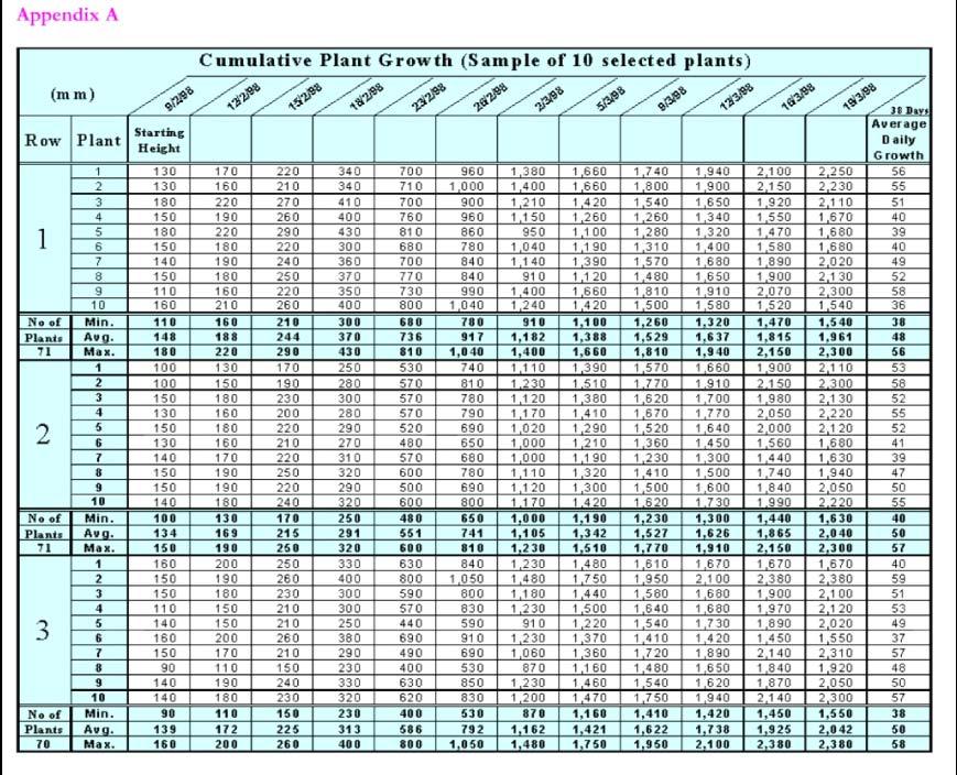
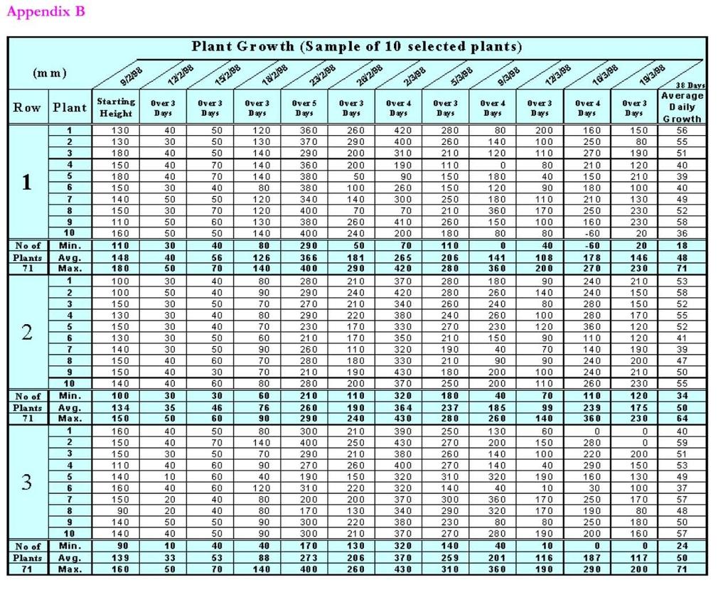
7 Test Results Plant Growth & Irrigation During the trial, the heights of the plants were measured at regular intervals, to obtain a comparison of growth rates between the treated and the untreated plants. The actual records of these readings are presented in the Cumulative Plant Growth, Appendix A. Appendix B contains the actual growth of the plants over the time between two sets of readings, where the interval is listed at the top of the table. For example, for plant number five in row two. When the trial was started, the plants were already 150mm high, 3 days later the plant had grown 30mm, 3 days later again it had grown 40mm and was now 220mm high. This plant had grown an average of 52mm per day over the entire trial period. Appendix C contains the average daily growth rates. This table is identical to that presented in Appendix B, except that the figure shown is the average per day over the interval between readings, whereas Appendix B was the total over that period. Each of these tables contains the minimum, maximum and average reading from each row of 10 selected plants. Comparing the average growth of the three rows in the trial as shown below, it becomes evident that the two trial rows were actually lagging behind in growth, up until after the 26/2/1998. This date is important, in that this is the date when the water delivery was corrected. It was found that the treated rows were not receiving sufficient amount of nutrient enriched water. The treated rows were purposely given less nutrient enriched water, as it was suspected that the treated plants required less water and/or nutrients. However, as it was noticed that the medium used to grow the treated plants were not as moist and had no run off. It was decided to increase the nutrient enriched water to the treated row.

8 Increasing the nutrient enriched water delivery to the treated rows produced the desired results as seen in the chart, Figure 6 by the increase in growth rate. This increase is also evident Figure 7 Figure 8, which compares the cumulative growth for each row. Each bar in Figure 7 is broken up into the minimum, average and maximum growth from the 10 selected plants. From this it also becomes evident that the minimum plant growth in the untreated row (1), exceeded the average growth of both the treated rows, up until the 26/2/1998. From this date, the chart also shows that the maximum plant growth occurs in the treated rows. Row 3 more so than row 2. From these charts, Figure 6 and Figure 8 we can with certainty say that the treated rows outgrew the untreated row. Studying the table Water Delivery Records in Appendix D, it is however obvious that even though the supply of nutrient enriched water to the treated rows were increased after the 26/2/1998, on average the treated plants still received less, almost 60ml less. This table of records contains three sets of water measurements, which were measured twice after the water delivery was corrected. The last water reading, on the 9/3/1998, showed that the nozzle to plant 7 in Row 2 was blocked, which had the effect of bringing the average delivery of row 2 down. The data, Table 2, extracted from Appendix D, also shows that, for this reading, the treated plants, row 3, on average received more water than did the untreated row, although one plant in the untreated row received 400ml, 10ml and 20ml more than rows 2 and 3 respectively. Due to that fact and the fact that, no further water measurements were taken, renders the three watering measurements inconclusive on their own. Hence, we cannot, with these measurements alone say that the increase in growth was due to variable water rate. Water delivery per plant per watering, 9/3/1998 (ml) Row Min Average Max However, we can to some degree of accuracy estimate the total amount of nutrient enriched water supplied to the treated rows. 1-Untreated Treated Treated The shade-house water delivery system was pumped through at a rate of 80 liters per minute as measured by the flow meter attached to the delivery line. This was always kept constant. This rate of water was delivered for a period of mostly 2 minutes and 45 seconds, although varied by the grower as necessary. Assume for the moment that this water delivery stays constant at 2minutes and 45 seconds. This will give a total of 2.75 times 80 liters or 220 liters of water for the entire shade house. The mark left by the nutrient enriched water in the charge tank used for the treatment was at a height of 165mm and the tank had a diameter of 560mm. Since the 40.6 liters were drained from the supply to the shade-house, that means that the remaining shade-house received liters or liters. When the grower changed the watering amounts, only the length of time would change, hence the division of water usage to the treated and untreated rows would vary proportionally.

9 The treated rows contained 141 plants of a total of 604 plants. This means that the treated plants would receive on average 288ml of nutrient enriched water per plant and the untreated plants would receive 387ml of nutrient enriched water per plant. If some plants received less than this quota, then another plant would receive more. Hence, on average the untreated plants received 34.4% more nutrient enriched water, yet the treated plants outgrew them. It is not so much that the treated plants became taller by about 4% on average, but that the rate at which they grew, as evident in Figure 8, provided that the nutrient and water supply is sufficient.

10 Nodes While studying and comparing the plants from separate rows, the grower noticed that the number of nodes from whence a fruit would grow were different between rows 1 (Untreated), 2 (Treated-Sawdust) and 3 (Treated-Coal Ash). Ten evenly spaced plants where then chosen from each row and the number of nodes were counted, as tabled below. When comparing these numbers it becomes quite evident that the treated plants produce on average an increased number of nodes, with an increase of about 20%, See Table 4. A greater increase was found on some of the treated plants, with an up to 32% increase. Perhaps more interesting is that the minimum number of nodes in the treated rows is only just less than the maximum number of nodes in the untreated row. This may be better demonstrated in the graph, Figure 9 With an increase in the number of nodes on each plant by about 20%, the potential of the plant to produce more fruit is increased. If we assumed that all the nodes were to bear fruit, then that would mean an increase in production of 20%. Fruit Abortions During the trial, a number of fruit throughout the shade-house aborted, meaning that the cucumber withered away after short time. It was noted that during a particular period of higher temperatures the plants aborted more fruit than usual and as a matter of interest for comparison, the number of fruit aborted were counted, as tabled in Table 5

11 It was suggested that the cause of this abortion was due to higher temperatures, during a summer period. When comparing the number of aborted fruit from each row, it was noted that the treated rows actually aborted more fruit than did the untreated row. Where rows 2 and 3 aborted 8.6% and 25.9% more fruit, respectively. Comparing this increase in fruit abortion to the increased number of nodes as shown previously. Should we hypothetically assume that all the nodes on every plant would bear fruit, then as shown in Table 6, we would have produced 1498, 1803 & 1764 cucumbers in Rows 1, 2 & 3 respectively. The amount of cucumbers aborted would be 220, 239 & 277 in rows 1, 2 & 3 respectively. With the remaining fruit being 1278, 1564 & 1487 respectively In the graph, Figure 10, each complete bar represents the hypothetical total number of fruit which rows 1, 2 & 3 would produce. The top area of each bar represents the aborted number of fruit. Hence the bottom section of each bar represents the remaining fruit. Studying these, it becomes evident that even though the treated rows lost more fruit, these rows would still be well ahead in fruit production. This is clearly demonstrated in Table 6 and Figure 10. As a percentage of each rowʼs production, the plants aborted 14.7%, 13.3% & 15.7% fruit for rows 1, 2 & 3 respectively. This percentage seems to be closely related. Yield The yield in this trial is the final measure of the success of the treatment. As such, every cucumber picked from the plants on all rows in the shade-house were recorded. The table of complete picking records is listed in the Crop Yield Records, Appendix E. Table 7, Table 8, Table 9 and are extracted from the table in Appendix E, which contain the picking records for the trial rows 1, 2 & 3 respectively, but also includes the cucumbers, which grew to a marketable size but were rejected by the grower for reasons of suitability.

12 In Table 7, we find that the row, which was picked to be the row for comparison (Row 1), produced 431 marketable cucumbers, with 305 rejected cucumbers. Compare that to Table 8, which are the picking records of row 2, treated and growing in sawdust and producing 617 marketable cucumbers and 319 rejected. Table 7 Table 8 Table 9, are the picking records of row 3, treated and growing in coal ash, producing 698 marketable cucumbers and 322 rejected cucumbers In terms of percentages, Figure 11, 41.4% is currently rejected from every plant. After the treatment, this is reduced to 34.1% in row 2 and 31.6% in row 3. To get an idea of the total yield, that is the Marketable plus the rejected cucumbers, refer to Figure 13, which shows a comparison of rows 1, 2 & 3, the trial rows. These numbers would seem to indicate that the treatment has increased the number of marketable cucumbers, without increasing the number of rejects proportionally, which may have been expected. This is clearly demonstrated in Figure 12 where the increase in cucumbers from row 1 to row 2 is 186 cucumbers with only 14 additional rejects and compared to row 3 with an increase of 267 cucumbers and only 17 additional rejects. Table 9 The bottom part of each bar in this chart indicates the marketable cucumbers and the top part the rejected. This clearly indicates that initially the untreated row (1) produced a better yield, however after the 15/3/1998; the treated rows outperformed the untreated row used for comparison. This chart also shows that row 3, produced a yield of 1020 cucumbers, row 2 with 936 cucumbers and row 1, the untreated only 736 cucumbers, that is ignoring the rejects, from which no financial gain could be achieved. However the plant still produced the fruit. If we study only the marketable cucumbers, as shown in Figure 13, which is just the top of the bottom section of each bar. Eliminating all other information we have Figure 14, which shows the marketable cucumbers throughout the trial. Again it is quite clear that the treated rows perform exceeding well.

13 Due to the fact that the row picked for comparison turned out to be the worst row, letʼs include each of the other rows in the shade-house. Rows 4, 5, 6, 7 and 8 produced a yield of 505, 520, 515, 488 and 481 cucumbers respectively. Figure 10, Marketed and reject yield Examining Figure 15, it becomes quite evident how bad the row chosen for comparison (row 1) actually was compared to the rest of the shade-house. However, this does not even take into consideration that each row has a different number of Figure 11, Season End Marketed and reject yield plants. Taking that into consideration, we get an average number of cucumbers per plant, however, this affects only rows 5 and 8, which have an additional 18 plants in each row.

14 This actually makes rows 5 and 8 worse than our control row, picked for comparison, with and average of 5.84 and 5.4 cucumbers per plant respectively compared to 6.07 per plant in row 1. Let us compare the average of the treated rows to the entire shade-house, Figure 1. Here we notice that on average the treated rows outperformed the entire shade-house by up to 3.6 cucumbers per plant and if sawdust was used instead of coal ash, 2.34 cucumbers per plant. Even if we were to include the two best rows in the shade-house, rows 4 and 6, with an average of 7.11 or 7.15 cucumbers per plant respectively. The treated rows are still ahead by 2.82 cucumbers per plant. Comparing each row average as a part of the entire shade-house, we notice that the treated row 2, makes up for 15% of the entire yield and row 3, 18% of the entire yield. The nearest competitive row is row 6 with 13%.

15 Rows 5 and 8 are as expected the worst at 9% and 10% respectively. This is due to the additional 18 plants in those rows. Studying the picking records as presented in Appendix E. We find that apart from the first picking on the 10/3/1998. The treated rows consistently produced a higher yield throughout the entire trial. This is perhaps more evident in Figure 13. Growerʼs Statement B & M Grorud On the 8/3/98 I began picking continental cucumbers from one of our hot houses. I was participating in an experiment conducted by Steven Walker. There were three rows of plants, Number one being the control row, number two being a row growing in a sawdust medium treated by magnetized water and number three being a row of coal ash medium also treated by magnetized water. During the growth stage of the plants I did notice the plants in the two magnetized rows seemed to be stronger and had a greener color to them as compared to the control row. Also the inter-node spacing was much closer on rows two and three. I did not have any deaths of plants in either of these rows as compared to the control row, which had quite a few. On picking I recorded all fruit Iʼd picked off all the rows. I found that row three had by far the most marketable amount of fruit with row two next in productivity and the control row with the weakest amounts. Row 3 - Produced 698 pieces of fruit Row 2 - Produced 617 pieces of fruit Row 1 - Produced 431 pieces of fruit It appears to me by this first experiment that the magnetized water treatment did have an influence on the performance of the plants and their productivity.

16 Yearly Yield Projection As this trial successfully shows, the treatment applied to the production of cucumbers has increased the growth rate and yield. The effect of which, if applied to an entire farm and not just a few rows is quite significant. If we use the production figures as shown in Appendix E for the entire shadehouse, excluding the treated rows, we would produce an average of 6.35 cucumbers per plant, compared to the 8.69 and 9.97 cucumbers per plant for the treated rows. In effect this means that if a hydroponic grower were to plant the crops in sawdust and treat the crop with the unit, the grower could expect in excess of 30% increase in yield. Should the grower utilize coal ash instead, then the increase in yield could exceed 50%. In terms of actual number cucumbers, see Table 10 or Figure 19. Yearly Yield Projection Treatment Average Cucumbers per Plant Number of Plants Untreated Treated - Sawdust Treated - Coal Ash Table 10, Yearly Yield Projection Say a grower s capacity is 20,000 plants per year. In this year, the grower can currently expect to collect around 126,998 cucumbers. If the entire yearly crop were grown in sawdust and treated then the grower could expect to collect 173,803 cucumbers, but should the grower utilize coal ash and subject the plants to the unit s treatment, then the grower could expect to collect around 199,429 cucumbers. That is, an additional 72,431 cucumbers.

17 Figure 19, Yearly Yield Projection Financial Projection To continue the example set out in the Yearly Yield Projection above, an additional 72,431 cucumbers per year at $0.60 each could produce an extra $43,458 per year to the grower of 20,000 plants. For farms of other capacities, please see Table 11 and Figure 20. Please note that this projection assumes no unforeseen effects from other factors such as extreme weather conditions or disease, which may or may not be mentioned in this report. It is merely a projection based upon the data collected during this trial. Full Year Financial Projection Treatment Average Cucumbers Per Plant Number of Plants Untreated 6.35 $19,050 $38,099 $57,149 $76,199 $95,248 $114,298 $133,348 $152,397 Treated - Sawdust 8.69 $26,070 $52,141 $78,211 $104,282 $130,352 $156,423 $182,493 $208,563 Treated - Coal Ash 9.97 $29,914 $59,829 $89,743 $119,657 $149,571 $179,486 $209,400 $239,314 Table 11, Financial Yearly Projection

18 Assuming that this projection is attractive, the next question will most likely be What will it cost the grower to implement the treatment on an entire farm?. Like most new installations, there is an initial setup cost. In this case the unit, capable of treating up to 10,000 gallons of water at a time, is the only additional expense. Ongoing expenses are minimal with just the weekly replacing of cost effective consumables. Based on the above projections any installations will have paid for themselves within a very short period of time. Figure 20, Financial Yearly Projection

19 Summary and Conclusion This trial has dealt with the application of the Bio-field treatment to that of a commercial crop of cucumbers. This treatment has involved a pre-charge of the nutrient enriched water, before delivery to the crop. The crop involved 8 rows of cucumber plants placed in a shadehouse, where only two rows were treated using the above mentioned device and one other row chosen for comparison, although a comparison with the remaining shade-house has also been performed. This document has compared observations of health, resistance or tolerance to disease and growth rates, but in particular, the number of nodes present on the plants resulting in increased yield and therefore increased profits. These observations were made, based upon the experience of grower. In terms of health, the treated plants were observed to be greener and generally healthier than the untreated plants. This is based upon observations made in regards to supporting stems, tip burns, leaves wilting, dead plants and color. Resistance or tolerance to disease was based upon the attack on the plants by a fungal leaf disease, where the treated plants were observed to cope more efficiently and remain greener and healthier for longer, even after the shade-house was sprayed. Looking at the fruit abortions, it has been made clear that all plants aborted fruit, and that the treated plants aborted more fruit compared to the remainder of the shade-house, when counted during a particular period of higher temperatures. However the treated plants also had more fruit to loose, as judged by the increased number of nodes. The treated plants produced up to 20% more nodes from whence a fruit would grow, at the time the nodes were counted. Throughout the trial, all plants randomly aborted fruit; however, no further attention was given to this. The treatment had the effect of increasing the growth rate of the plants. This was particularly noticed due to the initial lack of nutrient enriched water, which when corrected produced a significant growth in the treated plants. Regardless of the fact that on average they were still supplied with about 60ml less nutrient enriched water that did the untreated plants. Also interesting is that the treated plants were on average about 80mm taller. Finally, the reason for the trial, the increase in yield and hence profit. The treatment has increased the yield from an average of 6 to 7 marketable cucumbers per plant to an average of nearly 10 cucumbers per plant, which is an increase of about 57%. While the rejected cucumbers remained about the same across the rows, treated and untreated, this had the effect of reducing the fruit rejection from 41.4% to 31.6% Please note that this trial has been conducted in an actual commercial environment, where the judgment of the grower has been relied upon to vary conditions as necessary. This means that the plants were subjected to weather conditions and diseases as any commercial crop would and hence give a more accurate picture of the improvements provided by the treatment.

20

21

22