ABSTRACT RESPONSES OF THE COPEPOD ACARTIA TONSA TO HYPOXIA IN CHESAPEAKE BAY. Chesapeake Bay experiences seasonal hypoxia each year and while studies

Transcription

1 ABSTRACT Title of thesis: RESPONSES OF THE COPEPOD ACARTIA TONSA TO HYPOXIA IN CHESAPEAKE BAY Allison P. Barba, Masters of Science, 2015 Thesis directed by: Professor Michael R. Roman University of Maryland Center for Environmental Science Horn Point Laboratory Chesapeake Bay experiences seasonal hypoxia each year and while studies have been done investigating how the copepod Acartia tonsa responds to hypoxia, few studies have focused on a comprehensive understanding of how its behavior and fitness are affected by low oxygen. The abundance, distribution, fitness and diel vertical migration patterns of A. tonsa were measured on series of six cruises in 2011 and 2012 in spring, summer and fall. I found that copepod abundance, distribution and vertical migration were significantly affected when hypoxic waters occurred below the pycnocline. I also found that males were less impacted by hypoxia than females, with a greater decrease in female abundance and vertical migration when there were hypoxic bottom waters.

2 Responses of the Copepod Acartia tonsa to Hypoxia in Chesapeake Bay by: Allison P. Barba Thesis submitted to the Faculty of the Graduate School of the University of Maryland, College Park in partial fulfillment of the requirements for the degree of Masters of Science 2015 Advisory Committee: Professor Michael R. Roman, Chair Research Assistant Professor James J. Pierson Professor Diane Stoecker

3 TABLE OF CONTENTS List of Figures... v List of Tables...vi Chapter 1: Introduction... 1 Hypoxia... 1 Chesapeake Bay... 2 Hypoxia in Chesapeake Bay... 4 Zooplankton... 7 Acartia tonsa... 7 Acartia tonsa Diel Vertical Migration Acartia tonsa Response to Hypoxia Project Goals and Hypotheses Figures...16 Chapter 2: Acartia tonsa abundance, distribution and size in Chesapeake Bay Abstract Introduction Materials and Methods Cruise Timing Station Locations Collection Method Sample Analysis Statistical Analysis Results Hydrographic Data Acartia tonsa abundance and vertical distribution Acartia tonsa male and female distribution Acartia tonsa size distribution Discussion Acartia tonsa abundance and vertical distribution Acartia tonsa male and female distribution ii

4 Acartia tonsa size distribution Conclusions Figures Tables Chapter 3: Acartia tonsa migration in response to hypoxia Abstract Introduction Materials and Methods Collection Method Sample Analysis Calculations Statistical Analysis Results Acartia tonsa migration rate Acartia tonsa migration rate by Male and Female Acartia tonsa turnover rate Acartia tonsa turnover rate by Male and Female Discussion Acartia tonsa migration rate Acartia tonsa migration rate by Male and Female..64 Acartia tonsa turnover rate Acartia tonsa turnover rate by Male and Female Time of Day...66 Conclusions Figures Chapter 4: Conclusions Appendices Appendix A: Hydrographic Data Appendix B: Acartia tonsa abundance, vertical distribution and diel vertical migration.79 Appendix C: Species Diversity iii

5 References iv

6 LIST OF FIGURES Figure 1.1. Photo of Acartia tonsa Figure 2.1. Bathymetric map of Chesapeake Bay station locations 37 Figure 2.2. Photo of z-traps Figure 2.3. Five step diagram of sample collection methods Figure 2.4. Percent Acartia tonsa below the pycnocline versus partial pressure O 2 kpa..40 Figure 2.5. Percent of Acartia tonsa male and females below the pycnocline by cruise and station Figure 2.6. Ratio of male, female and copepodite above and below the pycnocline versus partial pressure O 2 kpa...42 Figure 2.7. Male and Female Acartia tonsa size versus temperature.44 Figure 2.8. Male and Female Acartia tonsa size versus partial pressure O 2 kpa...45 Figure 2.9. Male and Female Acartia tonsa size versus partial pressure O 2 kpa by cruise..46 Figure 3.1 Acartia tonsa migration rate vs partial pressure O 2 kpa and time of day..67 Figure 3.2. Male and Female Acartia tonsa migration rate over time...68 Figure 3.3. Male and Female Acartia tonsa migration rate vs partial pressure O 2 kpa.. 69 Figure 3.4. Acartia tonsa turnover rate vs partial pressure O 2 kpa and time of day..70 Figure 3.5. Male and Female Acartia tonsa turnover rate over time Figure 3.6. Male and Female Acartia tonsa turnover rate vs partial pressure O 2 kpa Figure A.1. Salinity data over date and time for all cruises.. 76 Figure A.2. Temperature data over date and time for all cruises Figure A.3. Density data over day and time for all cruises...78 v

7 Figure B.1. Acartia tonsa abundance separated by cruises and station Figure B.2. Acartia tonsa percent above and below by cruise and station Figure C.1. Species diversity by cruise vi

8 LIST OF TABLES Chapter 2 Table 2.1. Hydrographic data ranges for each cruise Table 2.2. Size range for male, female and copepodite Table 2.3 Statistical analysis for stepwise linear regression of size versus temperature and oxygen vii

9 CHAPTER 1: INTRODUCTION Hypoxia Hypoxia is defined as dissolved oxygen concentrations less than 2.0 mg L -1 (Diaz and Rosenberg, 1995). Anoxia is defined as 0.0 mg L -1 of oxygen. Seasonal hypoxia occurs in many aquatic habitats including estuaries, fjords, lakes and coastal systems. Hypoxia is often the result of high organic loading both natural and anthropogenic. Hypoxia is a natural process, but in recent years, occurrences have increased worldwide likely due to eutrophication (Diaz and Rosenberg, 1995). Eutrophication is the process in which high levels of nutrients, phosphorus and nitrogen, enter a system and stimulate a phytoplankton bloom. There are over 400 systems worldwide that experience eutrophication related hypoxia. Intensity and duration of hypoxia is dependent on many factors but probably most influential is nutrient loads entering the system. Depending on the residence time, whole system processes or mixing events, hypoxia can last from days to months (Diaz and Rosenberg, 2008). Freshwater brings large amounts of nutrients and organic matter into estuarine and coastal systems that stimulate a phytoplankton bloom. Zooplankton graze on the phytoplankton bloom but much of it remains uneaten. The dead phytoplankton and fecal matter sink to depths where bacteria feed on it. This process of decomposition by bacteria depletes the oxygen (Kemp et al., 2005). As this process continues, hypoxia develops. In many systems, bottom hypoxia can turn into anoxia. If anoxia is established, bacteria begin to produce hydrogen sulfide, H 2 S, which is toxic to many organisms. This usually happens in 1

10 systems with persistent hypoxia that occurs year after year with an accumulation of organic matter and nutrients in the sediments (Diaz and Rosenberg, 2008). Ecosystems that experience long periods of hypoxia have little to no benthic fauna and low secondary production. There is a decrease in energy transferred up to higher trophic levels. For example, in Chesapeake Bay, it is estimated that 5% of the Bay s total secondary production is lost because of hypoxia (Diaz and Rosenberg, 2008). Energy that should be moving from phytoplankton to higher trophic levels is instead flowing into bacterial pathways (Kemp et al., 2007). Habitat squeeze is also a possible issue in systems that experience hypoxia (Roman et al., 2012). Many animals, especially larger organisms such as fish, have a threshold for oxygen requirements and are unable to survive in hypoxic bottom water. Thus they are forced to reside in the oxygenated upper water column that may make them experience thermal stress as well as being more susceptible to predation. The goal of this thesis is to examine the effects of hypoxia on mesozooplankton, specifically the copepod Acartia tonsa. There are several studies that have focused on zooplankton response to hypoxia the results have been ambiguous and insufficient in situ work has been done. Chesapeake Bay The Chesapeake Bay watershed consists of 64, 299 square miles in the district of Columbia, Maryland, Virginia, Delaware, Virginia, West Virginia and 2

11 Pennsylvania (US Geological Survey, 2008). The Bay itself is 350 km long with a long central channel that is the original drowned river valley of the Susquehanna River. The channel depth varies but on average is 20 to 30 meters deep with broad shallow areas on each side of the channel. The deepest part of the Bay is 53 m but the average depth is 8.5 m (Kemp et al., 2005, Kimmel and Roman, 2004). The Bay is long and narrow and becomes broader and shallower as you move down bay towards the ocean. Because of the shape and size, Chesapeake Bay has a relatively long residence time of approximately 6 months. Temperatures range from 28 C in the summer to 2 C in the winter (Kemp et al., 2005). The Bay can be split into three distinct regions: 1.) The upper bay, or tidal fresh oligohaline portion, 2.) The mid bay, or mesohaline portion, and 3.) The lower bay or polyhaline section. There is a strong salinity gradient as you move down Bay, ranging from 0 at the head to 28 at the mouth. The salinity gradient controls organism distribution, primary and secondary production and biogeochemical cycles (Roman et al., 2005, Zhang et al., 2006). I will be focusing on the mesohaline section of the Bay because that is where hypoxia is often most severe. The Susquehanna, Choptank, James, Rappahannock, Patuxent and Potomac Rivers are the major freshwater inputs into Chesapeake Bay with the Susquehanna responsible for roughly 40% of the input (Roman et al., 2005). Freshwater discharge into the Bay drives the estuarine circulation in Chesapeake Bay. It also brings in nutrients and particulate materials into the Bay (Kemp et al., 3

12 2005). The plumes from the rivers have higher nutrient content than other areas of the Bay, which can increase the production and aggregation of phytoplankton and zooplankton. Freshwater inputs vary throughout the year with peak flows often occurring in the spring. This peak in flow influences the timing and magnitude of the spring phytoplankton bloom (Kimmel and Roman, 2004). Chesapeake Bay is a semi-enclosed estuary. The salty, dense water from the Atlantic Ocean moves up Bay along the bottom while the fresher, less dense water from rivers and streams remains at the surface as it moves down Bay. This creates two distinct layers, a saltier, denser bottom layer and a fresher, less dense surface layer, making Chesapeake Bay a stratified estuary (Decker et al., 2003). In the spring, during times of high freshwater flow, stratification becomes stronger. The Bay usually remains strongly stratified through summer and into fall until surface cooling and mixing events become more prevalent. Salinity and temperature are the major contributors to stratification in Chesapeake Bay creating a heavier, denser bottom layer and a less dense surface layer (Decker et al., 2003). The pycnocline is the horizontal layer where there is the greatest change in density. The depth and intensity of this layer shifts and changes depending on wind, waves, tidal currents and storm events (Keister et al., 2000). Throughout the course of a day, the pycnocline depth can become shallower or deeper in the water column. Depending on how weak or strong the pycnocline is, it could hinder vertical transport in the water column and mixing between the two layers (Keister et al., 2000). With less mixing, there is less oxygen reaching the bottom and this could enhance or prolong hypoxic events in Chesapeake Bay. 4

13 Hypoxia in Chesapeake Bay Chesapeake Bay experiences seasonal hypoxia. Freshwater flow, stratification, the shape and physical layout of the Bay, and anthropogenic inputs all play a role in the development of hypoxia (Keister et al, 2000). Like most systems, temperature, light and freshwater flow into the Bay increase in the spring, playing a major role in triggering the spring plankton blooms (Kemp et al., 2005). The plankton bloom is grazed upon by zooplankton but excess organic matter from the bloom, along with zooplankton fecal pellets sink to the bottom where it is broken down by bacteria. This decomposition by bacteria is an oxygen consuming process and oxygen in the bottom layer is quickly depleted (Kemp et al., 2005). In recent years, the duration and intensity of hypoxia has increased and anoxia has become more prevalent. Hypoxia occurs mainly in the deep channel of the Bay but had been observed to spread to shallower areas close to shore (Murphy et al., 2011). Oxygen depletion combined with Bay stratification sustains hypoxic conditions from June through September in most years. In some years, hypoxia develops as early as May and can last through September with anoxia developing periodically (Murphy et al., 2011). As oxygen decreases, a distinct oxycline develops that usually follows the pycnocline. In Chesapeake Bay, the retreat of hypoxia begins as fall approaches. Cooler weather allows the surface water temperatures to cool and wind and storm events increase allowing the two layers to mix which leads to the retreat of hypoxia (Diaz and Rosenberg, 2001). Although the duration of hypoxia in 5

14 Chesapeake Bay is relatively short term, the effects can be detrimental (Diaz and Rosenberg, 2001). Anthropogenic inputs have been linked to many areas that experience seasonal hypoxia. Chesapeake Bay is a large watershed and home to large cities such as Washington DC and Baltimore but also has a large area dedicated to agriculture. Heavily populated areas and farms treated with fertilizers are major contributors to the nutrients entering Chesapeake Bay (US Geological Survey, 2008). Historically, the Bay has been experiencing seasonal hypoxia since at least 1950 but the area affected by hypoxia has tripled since then (Kemp et al., 2005). Hypoxic events have become more intense and last for longer periods of time as the watershed has become heavily populated and land use has increased (Diaz and Rosenberg, 2008). It has been suggested that changes in the phytoplankton community and oxygen levels could lead to a shift towards planktonic food webs or bacteria and gelatinous zooplankton dominant ecosystem (Kemp et al., 2004). Mesozooplankton play an important role as the link between primary production and higher trophic levels. It is important to understand how hypoxia affects mesozooplankton in Chesapeake Bay because, although hypoxia dissipates in a few months, it can have devastating effects on the ecosystem. When this project began, we were using the standard definition of hypoxia in terms of dissolved oxygen <2 mgl -1 to determine the effects of low oxygen on Acartia tonsa. As the project developed and new information became available, we decided to use partial pressure of oxygen (po 2 ) rather than dissolved oxygen 6

15 measurements. Both partial pressure and diffusivity of oxygen in water are important because these properties determine the rate of oxygen uptake by organisms (Verberk et al., 2011). The solubility of oxygen in water is greater in cooler temperatures and lower salinities than at higher temperatures and higher salinities (Elliott et al., 2013). Using this definition rather than the standard hypoxia definition, we are able to take temperature into account since it can have a large impact on oxygen levels especially in the summer months. For the results and discussion of this project we used the partial pressure levels of oxygen that are stressful (P critical or P crit ) and fatal (P lethal or P leth ) to Acartia tonsa (Elliott et al., 2013). Zooplankton For this study, we focused on mesozooplankton, which have a size range from 200 um to 2mm. There are two species of copepod that are the most common in Chesapeake Bay, Acartia tonsa and Eurytemora carolleeae. We selected Acartia tonsa because they are the dominant zooplankton in the mesohaline section of the bay where hypoxia occurs (Kimmel and Roman, 2004). Zooplankton populations in Chesapeake Bay vary seasonally with different species dominating at different conditions. Acartia tonsa have two large blooms occurring in early spring and early fall closely following seasonal phytoplankton blooms (White and Roman, 1992). 7

16 Acartia tonsa Acartia tonsa is a calanoid copepod that that is widely distributed in estuarine and coastal environments. It is the dominant zooplankton species in the coastal Atlantic Ocean and estuaries from Massachusetts to Florida and in the Gulf of Mexico (Mauchline, 1998). Copepods, specifically Acartia tonsa, are the most dominant zooplankton in the mesohaline section of the Bay (Kemp et al., 2005). Acartia tonsa is most abundant in salinities between 5 and 30 but can be found in water with salinity as low as 1 in warmer temperatures. A. tonsa can tolerate temperatures from 0 to 30 C and are most common in depths of 0 20 meters (Johnson and Allen, 2005). Adult A. tonsa have an average generation time of 26 days but this can be as short as ten days in warm summer temperatures (Mauchline, 1998). They exhibit seasonal population fluctuations with highest abundances in warmer temperature months. Acartia tonsa reproduce via broadcast spawning, releasing fertilized eggs into the water column. Female A. tonsa can produce eggs for 3-4 weeks at a time and can release eggs per day (Mauchline, 1998). Eggs are spherically shaped and are µm in diameter. Egg hatching time is dependent on temperature but in warm temperatures, eggs can hatch within 24 hours (Mauchline, 1998). The eggs hatch as nauplii, the first larval stage for many crustaceans, and progress through six stages, N1 through N6, before becoming metamorphosing into copepodites. Copepodites then progress through six stages, C1 through C6, becoming mature adults in the sixth stage (C6) 8

17 (Mauchline, 1998). Adult A. tonsa are distinguished by an elongated prosome with a tapered head with the head about 50% of the total length. They have a single dark reddish colored eye and a short caudal rami with long fan like setae. Adult females grow to mm in length and males grow to mm. Males and females are distinguishable by their antennae, urosome and swimmerets (Johnson and Allen, 2005). Females have a visible single gonopore on the urosome and small fifth legs. Males have larger fifth legs and modified antennae used for mating. Adults can alternate between suspension feeding on immobile particles and ambush feeding on moving microzooplankton and phytoflagellates. They feed on phytoplankton, microzooplankton, and their own eggs and nauplii (Mauchline, 1998). White and Roman, 1992, found that Acartia egg production in Chesapeake Bay is not limited by food. Zooplankton feeding rates were more closely linked to temperature rather than food availability. Acartia use feeding currents to move food towards to their mouthparts where they are able to grasp the food and feed on it (Mauchline, 1998). They are discriminatory feeders in that they choose to feed on food of a specific size, shape and smell. They also select food based on quality, choosing faster growing algae with higher levels of carbon (Kiorboe et al., 1996). If an individual pulls a food item towards itself, it is able to choose to feed on the item or to reject the food item back into the water column and continue to forage for a more desirable food choice (Frost, 1972). Temperature also plays a role in copepod growth and development. Forster et al. (2011) define development as passing through life stages and 9

18 growth as the increase in mass. The rate at which nauplii and copepodites develop into adults is temperature dependent. Growth, or size, is also temperature dependent increasing with temperature and then levels off as temperatures reach an optimum level (Mauchline, 1998). Prosome length varies seasonally being larger in cooler months and shorter in warmer months. Calanoid copepod size has been found to be more temperature dependent than food dependent (Mauchline, 1998). Because we are capturing the animals at a developmental stage and preserving them, we are focusing on growth, or size, rather than development. Acartia tonsa are most prevalent in the middle portion of Chesapeake Bay where two key zooplankton predators are also highly concentrated: the ctenophore Mnemiopsis leidyii and scyphomedusae Chrysaora quinquecirrha. Other predators include juvenile striped bass (Morone saxatillis), white perch (Morone americana) and juvenile and adult bay anchovy (Anchoa mitchilli) (Zhang et al. 2006). Acatia tonsa play an important role in the aquatic food web. Copepods are the primary source of transferring primary production energy from phytoplankton to higher trophic levels. They are primary consumers that graze on phytoplankton and microzooplankton and are the primary food source for many juvenile and larval fish (Kemp et al., 2005). It is therefore important to understand how copepods, specifically Acartia tonsa, are behaving and responding to hypoxia in Chesapeake Bay so we can further understand and predict food web interactions. Acartia tonsa Diel Vertical Migration 10

19 Many species of zooplankton exhibit diel vertical migration patterns where they ascend to the surface at night and descend back to depths during the day (Ringelberg, 2010). At dusk, individuals move to the surface to feed on phytoplankton and microzooplankton and move back to depths around dawn where they fast during the day. It is hypothesized they do this to reduce risk of being visible to predators when it is light out. Many zooplankton species respond to light as a cue for migration patterns. Some species use temperature or density cues but it has more recently been observed that oxygen levels can be a cue to migrate (Ringelberg, 2010). Acartia tonsa are one of the many zooplankton species that exhibit diel vertical migration. They spend the daytime fasting at depths to avoid predation and migrate to the surface at night to feed (Roman et al., 1993). To move into the surface layer, they use a hop and sink movement to make the excursion to the surface layer. Through gut content analysis with Calanus species, it has been found that copepods moving into the surface have less in their guts compared to those moving out of the surface (Pierson et al., 2009). When food is scarce, it is likely that individuals remain at the surface for longer than if food was plentiful. With less food, it takes longer to feed to satiation leaving them at risk to predators when they remain at the surface past dawn. The same could be true when individuals are exposed to hypoxia (Hays et al., 2001). It is possible they are remaining at the surface for longer periods of time to avoid hypoxic bottom waters. Roman et al. (1993) found that few copepods remained in the hypoxic bottom layers making them more vulnerable to predation in the 11

20 surface layer. They observed that copepod numbers were highest in the pycnocline and surface layer and there was a disruption in diel vertical migration when oxygen was low (Roman et al., 1993). Acartia Response to Hypoxia Hypoxia can have negative effects on zooplankton fitness, fecundity and mortality (Decker et al., 2003). Low oxygen water can disrupt the vertical migration pattern. Numerous studies over the years have reported the negative effects low oxygen has on aquatic organisms specifically Acartia tonsa. It was observed by Roman et al. (1993) that zooplankton biomass is less in low oxygen bottom water than it is in normal oxygen conditions. During this study, copepods remained in the surface layer, just above the low oxygen water during the daytime. This could be putting copepods at risk for predation negatively impacting copepod abundance in the Bay. Taylor and Rand (2011) observed fish aggregations near the pycnocline taking advantage of the high prey densities. Their findings suggest that hypoxia causes a separation between plankton and juvenile fish creating increased competition for resources among fish. Zhang et al. (2006) saw similar results with reduced copepod numbers when the bottom layer had low oxygen present. Sedlacek and Marcus (2004) reported a decrease in egg production by Acartia tonsa when in low oxygen. They suggested that with reduced egg production in a given system, copepod numbers would decrease which may lead to a decrease in the species that rely on copepods for food. Elliott et al., (2013) 12

21 found that copepods remaining in low oxygen bottom waters have increased mortality and reduced growth and reproduction rates. They observed a greater non predatory mortality in Acartia tonsa nauplii when bottom layer oxygen was low also leading to the same conclusion as Sedlacek and Marcus (2004) that overall copepod numbers could decrease (Elliott et al., 2013). Studies have reported copepods absent from the bottom layer when oxygen is < 2 mgl - while others reported a change in depth distribution of copepods in low oxygen as a result in a disruption of diel vertical migration (Keister et al., 2000). It has also been observed that some species are more tolerant to hypoxia than others (Keister et al., 2000). Species such as the Bay anchovy, striped bass and naked goby, and copepods are not tolerant of low oxygen. Ctenophores, however, have higher predation rates under low oxygen conditions (Decker et al., 2004). These key copepod predators all exhibit avoidance behavior when low oxygen is present and move to areas with higher oxygen levels (Roman et al., 1993). This may alter zooplankton distribution and abundance in the Bay. It can also modify predation on zooplankton by larval fish and other predators (Keister et al., 2000). If predator-prey interactions are altered due to hypoxia, trophic pathways in Chesapeake Bay could shift. This could result in a change in predation rates, population densities and trophic pathways (Breitburg et al., 1997). While many studies exist on the topic of hypoxic effects on zooplankton abundance and distribution, fitness and diel vertical migration, there has yet to be any studies that look at all three comprehensively. 13

22 PROJECT GOALS AND HYPOTHESES This study was completed as part of the NSF Grant , Collaborative Research: Hypoxia in Marine Ecosystems: Implications for Neritic Copepods. The overall goal of the project was to develop a mechanistic understanding of how behavior and fitness of copepods, specifically Acartia tonsa, is influenced by hypoxia and how these effects are expressed in the population abundance, distribution and trophic dynamics. There were three overarching hypotheses investigated: 1.) Low-oxygen bottom waters exercise control over the vertical distribution and migration behavior of copepods, 2.) Lowoxygen bottom waters reduce the fitness of copepods and 3.) Low-oxygen bottom waters increase mortality rate by directly killing copepods and their eggs. In order to confirm that hypoxia is the main cause of mortality or decreased fitness of Acartia tonsa, we had to rule out other factors such as predation or lack of food as sources of mortality. This included investigating copepod egg production and mortality, phytoplankton communities, abundance and distribution of gelatinous zooplankton and larval fish, predation by gelatinous zooplankton and larval fish and the trophic link between phytoplankton, zooplankton and fish. If hypoxia does negatively impact zooplankton in Chesapeake Bay, there could be negative ramifications for other species in the Bay and ecosystem as a whole. The objective of my thesis was to investigate how low oxygen in Chesapeake Bay affects mesozooplankton populations, specifically the calanoid copepod Acartia tonsa. I focused on copepod migration behavior, abundance, 14

23 distribution and fitness under normoxic and hypoxic conditions. Based on the project hypotheses, I specifically investigated: Hypothesis one: Low oxygen water will reduce Acartia tonsa abundance and change thier distribution in the water column. In normoxic conditions, copepods are distributed throughout the water column. Under hypoxic conditions, it has been observed that overall abundances decrease and copepod populations remain above the pycnocline leaving themselves visible to predators (Keister et al., 2000). Hypothesis two: Low oxygen water will interrupt Acartia tonsa diel migration patterns leading to a decrease in copepods migrating. Copepods exhibit diel migration patterns in normal oxygen conditions. Under hypoxic conditions, they may avoid bottom low oxygen water or alter their typical migration patterns (Roman et al., 1993, Pierson et al., 2009). If they do avoid low oxygen water, this could disrupt migration patterns, subsequently disrupting feeding, reproduction and predation on A. tonsa by gelatinous zooplankton and larval fish. Hypothesis three: Low oxygen water will reduce the fitness of Acartia tonsa. Hypoxic bottom water may result in reduced copepod fitness through stress, a decrease in high quality food or a decrease in protein synthesis and metabolism. A decrease in copepod fitness could negatively impact copepod reproduction and 15

24 energy transfer to higher trophic levels. For this thesis I am using the term fitness to describe copepod size in relationship to temperature and oxygen levels. The subsequent chapters are intended to investigate these hypotheses to address our overarching project goal. Chapter 2 will address Acartia tonsa abundance, distribution and size/fitness and Chapter 3 will discuss Acartia vertical migration. Chapter 4 will synthesize the results from previous chapters and discuss the overall result of how A.tonsa responds to hypoxia and what broader implications, if any, these results could have on Chesapeake Bay food web dynamics. 16

25 Figures Figure 1.1. Acartia tonsa female (Photo credit James Pierson) 17

26 CHAPTER 2: ACARTIA TONSA ABUNDANCE, VERTICAL DISTRIBUTION AND SIZE IN CHESAPEAKE BAY ABSTRACT The marine copepod, Acartia tonsa, plays an important role in the Chesapeake Bay food web transferring energy from photosynthetic phytoplankton and microzooplankton to higher trophic levels such as larval and juvenile fish. Since Acartia tonsa are the most common copepod and an important food source in many coastal ecosystems, they potentially have a huge impact on the food webs. Chesapeake Bay experiences seasonal hypoxia but more recently, the volume of low oxygen water has increased dramatically. Studies have shown that copepods actively avoid low oxygen bottom waters and spend more time above the pycnocline and at the surface during times of low oxygen. With a focus on Acartia tonsa, we analyzed zooplankton samples that were collected on six cruises in Chesapeake Bay in 2010 and 2011, one each year in late spring, summer and early fall. All zooplankton species were counted and identified and Acartia tonsa was the most dominant zooplankton collected. We compared surface and bottom layer water column tows and contrasted the zooplankton communities and abundance. In many tows, overall abundance was lower in the bottom layer when oxygen was low but copepods were still present below the pycnocline. Females were more common in the surface layer than males when bottom layer oxygen was low, possibly due to higher metabolic needs of females. 18

27 INTRODUCTION The calanoid copepod Acartia tonsa is the most abundant zooplankton species in many coastal ecosystems including the mesohaline portion of Chesapeake Bay. Because of their large numbers, they play a vital role in food web dynamics of the systems they inhabit (Naganuma, 1996). Acartia are important grazer on phytoplankton and microzooplankton as well as a significant food source for many larval and juvenile fish, including the bay anchovy. Copepods are the main transfer of energy from primary production, phytoplankton, to higher trophic levels including larval fish (Kemp et al., 2005). The abundance, location and health of Acartia tonsa are major factors that can influence food web relationships in Chesapeake Bay (Johnson and Allen, 2005). Acartia tonsa are found most often in salinities between 5 and 30 but can be found in salinity as low as 1 when temperatures are warmer. Acartia can also tolerate a wide temperature range of 0 to 30 C and are most common in depths of 0-20 meters (Johnson and Allen, 2005). It has been observed that A. tonsa growth rate increases as temperature increases and then levels off at a certain point. Temperature is positively related to growth rate (Durbin et al., 1983). However, temperature and Acartia tonsa length are inversely related. As temperatures increase, length decreases (Durbin and Durbin, 1978). Acartia tonsa are one of the many copepods that broadcast spawn rather than carry their eggs. Females release their eggs in the upper layer of the water column where they will sink and hatch (Mauchline, 1998). Because this study took place during times of year when females are reproducing, this behavior 19

28 could impact where females are located in the water column. Hypoxia can have negative effects on zooplankton fitness, reproduction and mortality rates (Decker et al., 2003). Low oxygen water can disrupt vertical migration patterns and change the distribution patterns observed with higher oxygen levels. Zooplankton biomass is lower below the pycnocline when bottom oxygen levels are low (Roman et al., 1993). When copepods remain in the surface layer during the day, they put themselves at greater risk for predation. If they are actively avoiding low oxygen bottom waters, they are more visible to predators leading to a possible decrease in copepod abundance in the Bay (Keister et al., 2000). If there is a shift in copepod abundance or distribution, predation on zooplankton by larval fish and other predators could be altered negatively. With greater pressure on zooplankton from predators, copepods as a food source could eventually become depleted causing predators to rely on a lower quality food source (Keister et al., 2000). This chapter will focus on the abundance and distribution of Acartia tonsa above and below the pycnocline. I will determine the overall vertical distribution as well as male versus female distribution in relationship to oxygen. I will also report Acartia size in relationship to temperature and oxygen levels. MATERIALS AND METHODS Cruise Timing We conducted six cruises in the Chesapeake Bay, three cruises in 2010 and three Each cruise concentrated on a specific time period to capture 20

29 the seasonal stages of hypoxia. May cruises focused on the onset and development of hypoxia. The July/August cruises captured the effects of hypoxia after it has been established. The September cruises focused on the retreat and breakdown of hypoxia. Station Locations We selected two stations for the purpose of this study: a south station where hypoxia was less frequent and intense and a north station where hypoxia was more prevalent. The stations were selected based on hydrographic and water quality data collected using an undulating towed body (Scanfish) during the May 2010 cruise. We conducted an axial survey of Chesapeake Bay from north of the Bay Bridge to south of the Rappahannock River collecting temperature, conductivity, dissolved oxygen, fluorescence, and optical plankton data at onemeter intervals from the surface to approximately one meter off the bottom. The south station was located north of the mouth of the Rappahannock River ( W, N) and the north station was located near the mouth of the Little Choptank River ( W, N) (Fig 2.1). Both stations were located in the deeper main stem of the Bay with a depth of approximately 20 meters where hypoxia is more severe. The two stations differed in salinity but were similar temperature, biology and the copepod Acartia tonsa was the most dominant zooplankton. The same stations were sampled for the remaining five cruises. 21

30 Collection Method We collected zooplankton samples for 24 to 36 hours while at anchor at each station using two side-by-side nets with a 0.25 m 2 square opening and 200 µm mesh, deployed vertically with the mouth opening facing upward. The nets were designed by Pierson et al. (2009) to be used as traps to capture migrating copepods, with a single trip mechanism to close both nets at predetermined depths (Figure 2.2). We performed a series of zooplankton collections at four time periods: dusk, dawn, midday and midnight and repeated the series two to three times per time period. The collection series consisted of a vertical net tow from the bottom to the pycnocline, a vertical net tow from the pycnocline to the surface, a trap deployment with the same net that stayed stationary at the pycnocline for 45 minutes to capture migrators as they moved downward, a vertical net tow from the bottom to the pycnocline and a vertical net tow from the pycnocline to the surface (Figure 2.3). We conducted two or three trap series per time period. For example, at a given time period we would perform two net tows, a trap, two net tows, a trap, two net tows. Information from hourly CTD casts was used to capture the hydrographic data which was used to determine the pycnocline depth. Chesapeake Bay is a partially mixed estuary so there was often a sharp decline in oxygen at the pycnocline. For ease of graphing and demonstrating results, I put all of the traps and tows from a given station on a given cruise in chronological order, beginning with dawn and ending with midnight, which is not necessarily the order in which the 22

31 samples were collected. I did so to more easily show patterns between stations and cruises. However, this does not reflect the actual time we arrived on station and began collecting samples as these times varied for each cruise. For example, in May 2010 we arrived at the south at midnight and began sampling immediately but we arrived at the north station at midday and began sampling then. We calculated the volume of water filtered for the vertical net tows. In 2011, we used flow meter readings from a General Oceanics Environmental model serial #B flow meter to verify the calculated volume filtered. In 2010, when flow meter readings were not available, we relied on wire angle measurements. We required a wire angle under 25 degrees. The volume of water filtered for the traps should have been minimal because the traps remained at one depth for 45 minutes. Because we were anchored in one location for hours, multiple tidal changes occurred over that time causing tidal flow that affected the position of the nets in the water. When tidal flow or winds were high, the current would cause the nets to angle in the water creating the effect of a horizontal tow rather that the targeted vertical tow or trap. To resolve this, we had multiple solutions. First, we would add extra weight to keep the net stable in the water. If that did not solve the issue, we either did not use the sample, or if possible would redo the tow or trap as close to the original time frame as possible. After each tow and trap, we rinsed the nets thoroughly and concentrated the samples using a 200 µm sieve. We preserved from only one of the cod ends, in 4% buffered formalin to be identified and counted in the lab. The 23

32 second cod end was either used for lab experiments on board the ship or discarded. Sample Analysis The ICES Zooplankton Methodology Manual (2000) was used as a guideline for processing and counting the zooplankton samples. Since most samples were too large to count each organism, I counted a random 5 ml subsample of the entire sample collected using a Stemple pipette. I counted a minimum of 100 of the most abundance species from each sample, which in this case was always A. tonsa. Zooplankton in the subsample were identified down to the lowest taxonomic unit and the first fifty individuals were measured (prosome length and width) to determine the size distribution. I used the length and width measurements to compare fitness for adult male and female Acartia tonsa in each sample. I calculated zooplankton abundance (m 3 ) using the volume of water filtered and the total number of each species from the sample: Volume filtered (m 3 ) = net size (m 2 )*distance net moved through water (m) Total number = number in subsample*(dilution (ml)/subsample size (ml)) * 2 number of splits Abundance (individuals per m 3 ) = total in sample/volume filtered (m 3 ) Statistical Analysis Statistical significance for abundance below the pycnocline between the various oxygen levels was done using the Kruskal-wallis test. Due to the nature of the data, it failed the Kolmogrov-Smirnov and the Shapiro-Wilk tests for 24

33 normality so I was unable to use parametric statistical tests. The Kruskal-wallis test is a non-parametric test used for comparing two or more samples that are independent or have different sample sizes; it is the parametric counterpart to the ANOVA. Because this test is non-parametric, it does not assume normal distribution of the data, and uses a rank system to determine if samples are from the same distribution. I also used a non-parametric Friedman test to compare between different groups. We used a p=0.05 to determine if there was a significant difference between male and female data. Analysis was done using Matlab statistic toolbox. RESULTS Hydrographic Data Hourly CTD casts measured dissolved oxygen, salinity, density, and temperature throughout the water column (Table 2.1). Oxygen ranged from 0.02 mgl -1 at the north station in August 2010 to mgl -1 at the south station in September Oxygen levels were hypoxic or anoxic below the pycnocline at the north station during all cruises. Below the pycnocline at the south station, oxygen levels were hypoxic or anoxic at times during the August 2010 and July 2011 cruises. During all other cruises, oxygen levels at the south station were above hypoxic levels. Partial pressure of oxygen levels showed similar patterns to dissolved oxygen. PO 2 ranged from 0.05 kpa in August 2010 to kpa in September

34 Salinity and temperature varied between stations and between cruises. Salinity ranged from 0.37 at the north station in August 2010 to in August 2010 at the south station. The south station is located closer to the mouth of the Bay with a greater influence from the Atlantic Ocean therefore giving the south station higher salinity than the north station. In May and September 2011, salinity was lower than normal because of high rainfall in the spring and also in late August and early September. Temperature varied with the season. As expected, temperatures were highest in July 2011, at C at the north station and lowest in May 2010 and 2011, C and C, respectively. Density was lowest when salinity was lowest in August 2010 and also in May and September Density varied with salinity and temperature but salinity appeared to have a larger control over density (Appendix A.1 through A.3). Abundance and Vertical Distribution Acartia tonsa abundance and vertical distribution varied between station and season (Appendix B.1). Overall, the south station had a significantly higher abundance than the north station (Friedman p<0.05). At times, the north station had a higher surface or bottom abundance but the overall trend was higher numbers at the south station. The exception to this trend was in July 2011 where the north station abundance was consistently higher than the south station. Also, in September 2011 during the midnight tow series, higher numbers were 26

35 collected at the north station than the south station but these numbers were not significant. September 2010 had the highest abundances and August 2010 had the lowest. In 2011, May had the highest average abundances while September of that year had the lowest. During all cruises, Acartia were distributed throughout the water column and were found in both the surface and low oxygen bottom layer. Acartia were still present with oxygen levels below P crit and P leth. Total abundance fluctuated over time at the station and between stations and seasons. For each station, I calculated the percent of Acartia tonsa above and below the pycnocline based on the total amount collected in the water column to compare the distribution. It was difficult to conclude if abundance changed over time based on oxygen levels or if it was being influenced by tidal changes. As the tides change, water moves up and down Bay carrying zooplankton with it, so rather than use absolute abundance over time, I compared the top and bottom layers at each tow and time frame. The time between the tows was minimal and this was done to remove the variation of tidal changes but we cannot be confident when comparing two different time frames. This would not completely avoid the issue of tidal influence but it made it possible to compare the abundance between the two layers at a given time. For the results in this section, I am focusing on the percent of the total population below the pycnocline rather than absolute numbers above and below. Figure 2.4 shows the percent of Acartia tonsa population below the pycnocline compared to the partial pressure of oxygen. This graph is separated out when 27

36 bottom layer oxygen levels were Pnorm (above P crit levels), P crit and P leth to illustrate the distribution and abundance compared to oxygen. With O 2 levels below P crit and P leth levels for Acartia tonsa, we did not expect to see Acartia present but there were times when more than 50% of the population is in the low oxygen bottom layer. This means that when oxygen was at the lethal levels, more than 50% of the copepods at that time point were found below the pycnocline. At P norm levels, Acartia below the pycnocline ranged from 10-97%. At P crit and P leth levels the percent of Acartia below the pycnocline ranged from 13-96% and 2-80% respectively. Regardless of oxygen levels, we found that individuals were present below the pycnocline. However, after running statistical analysis of the percent below the pycnocline compared to oxygen level, the abundance above P crit was significantly higher than the abundance between P crit and P leth which were both significantly higher than the abundance below P leth (Kruskal-Wallis, p <0.01). In the May and September cruises of both 2010 and 2011, Acartia were found above and below the pycnocline the north and south stations (Fig B.2). Many times, percentages were similar or higher below the pycnocline compared to the surface regardless of the oxygen levels. Even when oxygen levels dropped below P crit or P leth, Acartia were still spread out throughout the water column. I observed a different pattern at the north station in August and July when oxygen levels were lowest reaching P crit and P leth levels (Fig B.2). Acartia tonsa did not completely avoid the sub-pycnocline layer as expected during the summer cruises but numbers were often lower in the bottom than in the surface 28

37 layer. With the exception of three tows in August 2010 and two tows in July 2011, there was a higher percentage of Acartia in the surface layer than in the bottom layer. In August, the tows were at dusk while in July the tows were at midday. Because oxygen levels were was so low in July 2011, the south station had bottom oxygen levels periodically fall below P crit and P leth causing Acartia percentages to be greater in the surface layer for all but two times, once at dawn and once at midnight (Fig B.2). Similar to the north station summer results, Acartia were still present in the bottom layer but in much lower numbers when compared to the surface layer, demonstrating avoidance of the layer. August and July CTD data showed little to no change in pycnocline depth or salinity and density in the water column before the times periods sampled which confirms that a change in tides was not likely the cause of high abundance in the bottom layer (Fig A.2 and Fig A.3). Acartia tonsa Male and Female Distribution To further determine zooplankton distribution in the water column, I separated out Acartia tonsa males and females below the pycnocline when PO 2 levels were below P leth (Fig. 2.5). Even with oxygen levels fatally low, over 40% of males were still found in the bottom layer at times. Below the pycnocline males ranged from 9-41% while females ranged from 6-36%. Although numbers are similar, the average percent below the pycnocline for all tows for males is 29% while it is 16% with females. 29

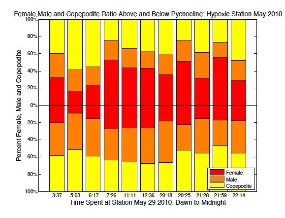
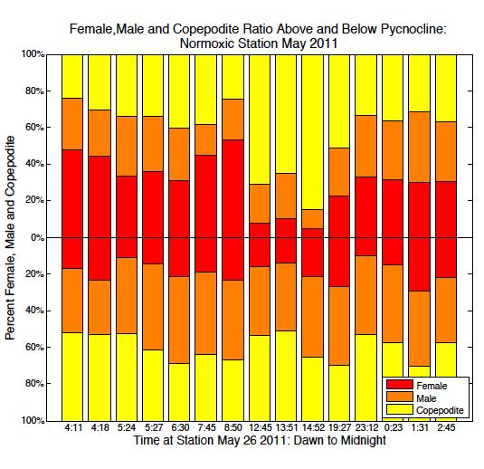
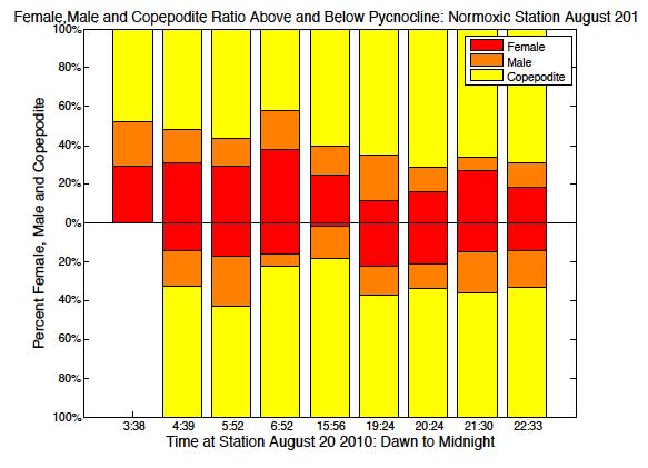
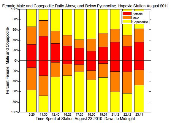
38 After calculating total abundance and percentage of Acartia tonsa above and below the pycnocline, I determined the percent of male, female and copepodite of total individuals collected in each net tow for both above and below the pycnocline (Fig 2.6). With the understanding that total abundances varied throughout the cruises, I wanted to determine what percent of each tow was male, female and copepodite. The overall trend shows a higher percentage of females in the surface layer regardless of station or season. Above the pycnocline, the average of all tows showed that females made up 29% of sample and males made up 20%. Below the pycnocline, on average, females compromised 14% of the population while males made up 32%. Females made up a significantly lower percent of the population below the pycnocline (Friedman p<0.01). Females were present above and below the pycnocline but were in higher percentages above the pycnocline. This trend was evident at both the north and south station but was more pronounced at the north station. Females often dominated surface layer samples comprising up to 80% of the sample. Male percentages varied over time and cruise with no clear pattern. There is no trend during a specific season or time frame at the station but rather they are spread out above and below the pycnocline. Copepodites also did not show a specific pattern but I did observe them at times making up a higher percentage of the sample at the north station. 30

39 Acartia tonsa Size Distribution As described in the methods, I measured the first fifty individuals of each sample. Many of the first fifty measured were Acartia tonsa and with this data I was able to compare sizes of male and female between stations for each cruise. Copepodite measurements were recorded but since they vary greatly between the C-1 and C-5 stages it was difficult to make any comparisons with that group. I calculated the length and width ranges of males, females and copepodites for each cruise to give an idea of the overall population during that time of that cruise (Table 2.2). Male and Female size varied with cruise and station. I averaged the sizes for each cruise and station to see if there was an overall trend. Male Acartia were larger at the south station for the spring and fall 2010 cruises but similar in size at the north and south station for the summer cruise. Females were larger for all 2010 cruises at the north station opposite to the male trend. The same was true for females for the spring and summer cruises in 2011 with larger averages at the south station while males were very close in size for the north and south stations. Both males and females were larger in in the fall of 2011 at the south station (Table 2.3). With so many data points, it was difficult to determine how size, if at all, varied with oxygen level. For this purpose, I used an average male and average female size for each net tow. To first rule out temperature being the control on size, I compared average size versus temperature (Fig 2.7). As expected, size varies with temperature. There was a threshold between C where there is 31

40 a distinct drop in Acartia length for both males and females. Below C female size ranges from mm and male size ranges from mm. Above the threshold temperature, females range from mm and males range from mm. There is a pattern of larger individuals, both male and female, in cooler temperatures and when temperatures increase, size decreases. We also hypothesized to see a trend where individuals were smaller as oxygen decreases. This trend was evident but we observed no significant pattern (Fig. 2.8). There is a slight increase in size when PO 2 is above 20kPa and the pattern is more obvious in males than females. With females, the data is varied but with males you can see a pattern where size increases with high levels of oxygen. Below and above 20kPa for PO 2 female size ranges from mm and mm respectively while males range from mm and respectively. The difference in size for both males and females was small and not as evident as with temperature. When I separated the data out by cruise and compared it to oxygen, sizes were not significantly different between seasons. May 2010 and 2011 copepods were largest with August 2010 and July 2011 being the smallest (Fig 2.9). This coincides with the trend I observed with temperature: larger individuals in cooler temperature months and smaller individuals in warmer temperature months. Although these trends were evident, I found that there was not a significant relationship (linear regression, table 2.4) between size and temperature, size and oxygen or size temperature and oxygen combined. 32

41 DISCUSSION Acartia tonsa abundance and vertical distribution Total abundance of Acartia tonsa varied with station and cruise with a general trend of seeing copepods in both the surface waters and below the pycnocline. We saw a higher total abundance during the fall and spring months with the lowest total abundance below the pycnocline during the summer cruises. Also when looking at the percentage of Acartia tonsa above and below the pycnocline, we observed a larger percentage above the pycnocline than below when oxygen was below P leth and P crit. When oxygen was above P crit, copepods were spread out above and below the pycnocline. When oxygen levels were above P crit and P leth and the percent of copepods in the bottom layer was higher than when oxygen was below P leth. When oxygen levels were below P leth levels, copepods were often in lower numbers below the pycnocline than above. This supports our hypothesis that low oxygen water will affect Acartia tonsa abundance and distribution. It was much less obvious than we initially expected and not statistically significantly but there was a trend showing a change in abundance in the bottom layer during times of low oxygen. Many studies show copepods completely avoiding the bottom layer or only dead copepods present in low oxygen levels. We found that even with levels below P leth, all stages of Acartia tonsa were present and alive. While abundance was lower below the pycnocline, copepods were still present. Due to the nature of our nets, we sampled only two layers, bottom to pycnocline and pycnocline to surface. While our results show that copepods were 33

42 present in the bottom layer, we are unsure where in the bottom layer they are located. For example, we are unable to determine if they are doing one of three things: 1.) Staying at the very bottom where oxygen is below P leth, 2.) Staying near to the pycnocline where oxygen is closer P norm or 3.) They are moving throughout the layer where oxygen levels vary. It is possible that copepods are simply surviving in low oxygen or it could be that all three situations were occurring but we were unable to capture it due to the nature of our sampling technique. As part of the project we also performed MOCNESS (Multiple Opening and Closing Net Environmental Sampling System) tows. When comparing our net tow data to the MOCNESS tows, we are able to see the same trends but with more detail since the MOCNESS sampled three to four layers rather than two (Katherine Lui, personal communication). The data from these tows support the idea that copepods are staying near the pycnocline where oxygen is closer to P norm. When comparing bottom layer tows to tows just below the pycnocline and in the pycnocline, total abundance (number per m 3 ) is lower in the bottom layer tows. These results show that copepods in Chesapeake Bay can be present in low oxygen. If copepods are able to survive in low oxygen, they are able to remain below the pycnocline staying hidden from predators during the day. Further studies could investigate how healthy copepods are in low oxygen and if they simply surviving or if they are actually thriving as they would in normal oxygen levels. 34

43 Acartia tonsa Male and Female Distribution We saw the general trend of more females than males in the surface layer. Females were in much higher numbers than males for most surface layer tows and a higher average percentage for the surface tows. This trend was something we had not predicted, but after seeing how pronounced it was, I developed two possible hypotheses as to why we saw this. The first hypothesis is that all cruises were done during a time when females are reproducing and are staying at the surface to release eggs. Usually females release eggs around dawn where the eggs sink and hatch into nauplii (Mauchline, 1998). This doesn t account for the high numbers during the day unless they are migrating to the surface layer to feed and then are remaining at the surface for longer periods of time until the eggs are ready for release. The other hypothesis is that females have higher metabolic needs requiring them to stay out of low oxygen bottom waters for periods of time. Females are larger than males so it is possible that they require higher levels of oxygen and are less tolerant of low oxygen. With the cruises occurring during spawning season, they could have higher feeding rates or higher oxygen needs while producing eggs. It could also be that females require higher quantities of food and stay in the surface layer where food concentration is higher. Although we are unsure as to why we saw this trend, we know the trend exists and it is very apparent throughout all cruises. This is a topic that future studies could focus on to see if this is something we would see year round and is 35

44 a general trend for Chesapeake Bay and other systems or if this is only a trend we would see when bottom layer oxygen is low. Acartia tonsa size distribution We also saw that oxygen was not the main control on Acartia tonsa size. Our results show temperature has a greater influence on copepod size than oxygen. Males and females were larger in cooler temperatures than when at higher temperatures. Sizes of copepods found below P crit or P leth copepod did not vary as we had expected. It is not until oxygen levels were well above P crit levels that copepod size increases and even then, the change in male and female size is small. There is a slight jump in size when oxygen levels were high. It is difficult to completely separate the relationship between size and temperature and size and oxygen since low oxygen often occurs with higher temperatures. Also, since copepods vertically migrate, they are likely spending only part of their day in low oxygen waters so the effect of oxygen on size may not be apparent. We observed that males were more spread out above and below the pycnocline and were in higher numbers than females in the bottom layer. This distribution could be having a greater effect on males since females are spending more time at the surface layer out of the low oxygen layer but further research is needed. These results support do not support my third hypothesis: Low oxygen water will reduce the fitness of Acartia tonsa. When bottom level oxygen is below P crit or P leth levels, copepods could become stressed which may reduce 36

45 their fitness or size. My results show little relationship between size and oxygen but it does show male size was more influenced by oxygen than female size. This could lead to a decrease in the quality of food available for juvenile and larval fish affecting their growth and development. Less healthy copepods could lead to a chain reaction up the food web causing a less healthy ecosystem. Further studies are needed to determine a better understanding of the relationship between size and oxygen with a more detailed focus on fitness ratios and oxygen. 37

46 CONCLUSIONS The objective of this study was to determine the effect, if any, low oxygen has on Acartia tonsa abundance, distribution and size in Chesapeake Bay. We found that low oxygen does have an impact on copepods abundance and distribution in the water column especially when oxygen levels were below P leth. However, we did find that low oxygen did not completely deter them from remaining in the bottom layer for protection from predators during the day and night. Low oxygen showed to be more restrictive for females while males were able to survive in the bottom layer. There was a slight increase in male size when oxygen levels were high with less of an impact on female size. We were unable to conclude how low oxygen affects copepod size but deeper investigation into this topic may reveal a similar result to abundance and distribution. Copepods are food for many juvenile and larval fish as well as help control and limit phytoplankton and microzooplankton communities in many ecosystems worldwide. Acartia tonsa in Chesapeake Bay is a key species that plays a complex role in the food web. They account for a large portion of the food for many organisms in the mesohaline section of the Bay. With these results, we gained a better understanding of how copepods respond to low oxygen and can take a deeper look to determine how low oxygen could affect the Chesapeake Bay food web. 38

47 FIGURES Figure 2.1. Bathymetric map of Chesapeake Bay station locations 39

48 Figure 2.2. Photo of z-traps (credit James Pierson) 40

49 Figure 2.3. Five step diagram of sample collection method 41

50 Figure 2.4. Percent Acartia tonsa below the pycnocline versus partial pressure O 2 kpa 42

51 Figure 2.5. Percent of Acartia tonsa male and female below the pycnocline versus partial pressure O 2 kpa below P leth 43

52 May South May North August/July South August/July North

53 September South September North Figure 2.6. Ratio of male, female and copepodite above and below the pycnocline over time from dawn through midnight. Blank spaces represent no data available. 45

54 Figure 2.7. Male and Female Acartia tonsa size versus temperature 46

55 Figure 2.8. Male and Female Acartia tonsa size versus partial pressure O 2 kpa 47

56 Figure 2.9 Male and Female Acartia tonsa size versus partial pressure O 2 kpa by cruise 48

57 Dissolved Oxygen (mg/l) May 2010 North South North South North South Aug 2010 Sept PO 2 (kpa) Salinity Temp ( C) Density (kg/m^3) Dissolved Oxygen (mg/l) May 2011 North South North South North South July 2011 Sept PO 2 (kpa) Salinity Temp ( C) Density (kg/m^3) Table 2.1. Tables of hydrographic data ranges for each cruise 49

58 May 2010 August 2010 September 2010 Male (mm) North South North South North South 0.770± 0.820± 0.709± 0.709± 0.713± 0.730± Female (mm) 0.935± ± ± ± ± ± Copepodite (mm) 0.546± ± ± ± ± ± May 2011 July 2011 September 2011 Male (mm) North South North South North South 0.777± 0.778± 0.725± 0.720± 0.715± 0.752± Female (mm) 0.924± ± ± ± ± ± Copepodite (mm) 0.581± ± ± ± ± ± Table 2.2. Table of size range for male, female and copepodite 50

59 Female Male Female Male Female Male 7.06 e e e Female Male Female Male Female Male e e -08 Table 2.3 P values for ANOVA analysis comparing male and female size between stations for each cruise p-values for: Temperature Oxygen Temperature and Oxygen interaction Female Male Table 2.4. P values for stepwise linear regression analysis comparing male and female size with temperature, oxygen and the combined effect of temperature and oxygen. 51

60 CHAPTER 3: ACARTIA TONSA MIGRATION IN RESPSONSE TO HYPOXIA IN CHESAPEAKE BAY ABSTRACT Copepods exhibit diel vertical migration rising to the surface at dusk and descending to depths at dawn. Diel vertical migration has long been observed as a survival strategy for copepods. Many studies have shown that when oxygen levels are low, diel vertical migration patterns are disrupted. This study focused on diel vertical migration patterns over a period of six cruises in 2010 and We collected samples at both dusk and dawn to attempt to capture diel vertical migration as well as midday and midnight to determine if there is movement at other times of day. I identified and counted Acartia tonsa present in the samples and calculated the number of individuals migrating across the pycnocline, or migration rate (m -3 h -1 ), and also the percent of the Acartia tonsa population migrating across the pycnocline between layers, or turnover rate. Our results show the most movement out of the surface layer at midnight rather than at dawn as expected. The least amount of movement was at midday with various amounts of movement at both dusk and dawn. We found that low oxygen didn t completely deter copepods from migrating and we did observed large movements out of the surface layer across the pycnocline. We also observed a difference between male and female migration patterns when oxygen was low. 52

61 INTRODUCTION Many species of zooplankton exhibit diel vertical migration or DVM. In both fresh and salt water habitats, individuals rise to the surface at dusk and descend to the depths during the day. Different species move various distances ranging from a few hundred meters to tens of meters. Copepods are one of the many organisms that exhibit this behavior (Ringelberg, 2010). They ascend to the surface at night to feed on phytoplankton and microzooplankton. They have been observed to remain in the surface layer until dawn where they will descend back to depths. They spend the light hours at depths where they are less visible reducing the risk of predation by juvenile and larval fish (Ringelberg, 2010). Acartia tonsa are one of the many zooplankton species that exhibit this behavior. They are a dominant zooplankton species in many aquatic ecosystems and are the most prevalent copepod species in the mesohaline section of Chesapeake Bay. Acartia have been observed to spend the daytime fasting at depths to avoid predation and then migrate to the surface at night to feed (Roman et al., 1993). Hunter and Brooks (1982) found that when food is limited, individuals spend more time at the surface than when food is abundant. They hypothesized that the same could be true for when individuals are exposed to hypoxia. It is possible that Acartia tonsa remain at the surface for longer periods of time to avoid hypoxic bottom waters. Research has shown that copepods often do not remain in the bottom layer and avoid hypoxia, instead, spending more time in the 53

62 surface layer making them more visible and susceptible to predation (Roman et al., 1993). Hypoxia has been observed to negatively impact copepod fitness, reproduction and mortality and alter copepod diel vertical migration patterns (Decker et al., 2003). When bottom layer oxygen is below normal oxygen conditions, zooplankton biomass is lower in the low oxygen water than the water above it. Acartia tonsa were found in high densities at depths when oxygen levels were high but were consistently absent from the same depths when oxygen levels were low (Roman et al., 1993). Copepods may remain in the surface layer and pycnocline to avoid low oxygen, but this puts them at risk for predation. It has also been hypothesized that when hypoxia is severe, the pycnocline acts as a physical barrier between the bottom and surface layer preventing vertical migration. Many species such as Bay anchovy, naked goby, striped bass, and copepods are less tolerant of low oxygen than other species (Keister et al., 2000). They exhibit an avoidance behavior when oxygen is low and move to areas with higher oxygen. This allows for a habitat squeeze to occur with more individuals in a smaller area because only a portion of the Bay has oxygen levels adequate for these species. With a crowded habitat, encounter rates are increased, leading to higher predation on copepods. Roman et al., 1993 also observed that when bottom layer oxygen was low, copepods migrated a shorter distance in the water column and avoided the hypoxic bottom layer. 54

63 When copepods diverge from their normal diel vertical migration patterns, there could be negative impacts for the ecosystem. If copepods remain at the surface to avoid low oxygen, they will be at a higher risk for predation (Kimmel et al., 2006). This could alter copepod distribution and abundance in the Bay and have negative impacts for the food web. With more copepods available in the surface layer, it could be possible that predators are feeding on a greater number copepods than when oxygen levels are normal, ultimately leading to fewer copepods available as a food source (Keister et al., 2000). Diel vertical migration is an important behavior for copepods to display because it allows for them to actively feed at the surface night while remaining hidden at depths during the day. With a disruption to these patterns Chesapeake Bay could experience a decrease in Acartia tonsa populations due to increased predation at the surface or nutrient deficient copepods for higher trophic levels. This would have adverse impacts for the food web resulting in negative effects for the whole ecosystem. This chapter will focus on Acartia tonsa diel vertical migration patterns at four time periods: dawn, midday, dusk and midnight during six cruises in 2010 and I will determine patterns of migration in relationship to oxygen level and time of day to see how low oxygen impacts copepod DVM. 55

64 MATERIALS AND METHODS Collection Method The collection method for this chapter is the same as described in Chapter two on pages 17 through 22 with emphasis on the trap collections. See figure 2.2 for a detailed description of sample collections methods. We are focusing on the trap samples for this chapter (step 3 in Fig 2.2) but the vertical tow samples are used for calculating migration rate and percent turnover. After the two vertical net tows, we placed the nets in the water for forty-five minutes with the net opening set at the pycnocline. At the end of the forty-five minutes, we closed the nets using a brass messenger and net trip mechanism and brought them onboard for preservation in formaldehyde. We preserved one of the two cod ends for enumeration in the lab. Both flow meter readings and wire angle measurements were taken into account when calculating migration rates. We excluded samples where flow meters measured significant amounts of water moving across the net opening or when the wire angle was greater than 25 degrees. In these cases, the stationary net was acting as a tow and filtering water, rather than only trapping migrating copepods. When this was the case, we attempted to rectify the situation by adding extra weight to the net and if that did not solve the issue, we either excluded the data from that sample, or when possible we would redo the trap as close the original time as possible. 56

65 Sample Analysis The sample analysis for the migration data is the same as described in chapter two on pages 20 through 22 following the same guidelines as described in ICES Zooplankton Methodology (2000). The first fifty zooplankton from the trap samples were counted, identified and measured and the remainder of the sample was counted and identified down to the lowest taxonomic unit. The focus of this analysis was only Acartia tonsa, where as with the tow samples when were looking at the entire zooplankton community. Calculations Using the data from the trap samples and surface layer tows shown in chapter 2, I calculated copepod migration rates between the two layers. We defined migration rate for Acartia tonsa as the number of individuals crossing the pycnocline moving from the surface layer into the bottom layer over a period of time. We calculated all rates as individuals m -3 h -1. Values for migration rate could have been either positive or negative, where positive values meant more individuals were moving into the surface layer than out of the surface layer and negative values meant more individuals were leaving the surface layer than moving into it. Migration rate can be calculated following the method by Pierson et al., 2009: Migration Rate (individuals m -3 h -1 ) = A f A i - A t i t nets 57 D*t traps Where: A f = abundance of Acartia tonsa in the upper layer after the trap (m -3 ) A i =abundance of Acartia tonsa in the upper layer before the trap (m -3 ) A t = abundance of Acartia tonsa in the trap sample (m -2 )

66 t nets = amount of time between net tows (h -1 ) t traps = duration of trap deployment (h -1 ) D = depth of the trap deployment (m) To calculate the turnover rate, which is an estimate of the percent of the copepod population at a given time point migrating across the pycnocline, I used the method from Pierson et al. (2009). The migration rate measures how many copepods are moving between the surface and bottom layers over a period of time (individuals m -3 h -1 ). The turnover rate differs in that it finds the percent of the Acartia tonsa population moving out of the surface layer during one trap time period. In other words, how much of the total A. tonsa population at that time point are moving from the surface layer down to the bottom layer. To calculate turnover rate, I divided migration rates (m -3 h -1 ) from a trap sample by the average concentration (m -3 ) in the surface layer tows that were taken before and after the trap. Turnover rate (%)= Migration rate/ (A b +A a /2)*100 Where: Migration rate (from above) = (m -3 h -1 ) A b =Abundance of copepods in surface tow before trap (m -3 ) A a =Abundance of copepods in surface tow after trap (m -3 ) Statistical Analysis As with the tow data, the trap data failed tests for normality and I was unable to use a parametric test for statistical analysis. I opted for the Kruskalwallis test to determine statistical significance between the migration rate and turnover rate in comparison to oxygen level and time of day. I also used the Friedman test to determine statistical significance, if any, between males and 58

67 females for both migration and turnover rate in relation to oxygen and time of day. I used a p-value < 0.05 to determine statistical significance. Analysis was done with Matlab using the statistics toolbox. RESULTS Acartia tonsa Migration Rate The largest migration rates were recorded between dusk and midnight (Fig 3.1). There was a significant difference between migration rate and time of day (Kruskal-Wallis, p=0.0331). There were significantly higher migration rates recorded at midnight over dusk, dawn and midday. I found similar migration rates at dusk and dawn with the lowest rates of movement at midday (Fig 3.2). There were higher measurements recorded at dusk and dawn but large movements during midday traps were not frequent. Our results show copepods moving into the surface layer at dusk with large movement at midnight rather than at dawn as we had expected based on previous studies. Overall migration rates ranged from 49,280 individuals m -3 h -1 to -521,467 individuals m -3 h -1. There was no significant difference between the above P leth and below P leth migration rates (Kruskal-Wallis, p=0.1806). Individuals are moving between layers regardless of oxygen level but we did observe a trend of decreased migration rates when oxygen is low. The largest movements occur when oxygen levels were above P leth with smaller migration rates when oxygen is below P leth (Fig 3.3). When above P leth, I calculated a range of 49,282 to -521,467 59

68 individuals m -3 h -1. When oxygen was below P leth, I calculated a range of 19,368 to -115,827 individuals m -3 h -1. Acartia tonsa Migration Rate by Male and Female Both male and female migration rates varied with oxygen level (Fig 3.3). Female migration rates range from 6,495 to -194,528 individuals m -3 h -1. Male migration rates range from 8,325 to -191,520 individuals m -3 h -1. There is a significant difference between male and female migration rates when oxygen levels are below P crit (Friedman test, p=0.0066) but not when oxygen is above P crit (Friedman test, p=0.6310). Male migration was significantly higher when oxygen was below P crit. Previous studies report that the largest migration rates into the surface layer should be around dusk and the largest movement out of the surface layer should be around dawn. We observed the largest movements out of the surface for both males and females during the dusk and midnight trap sample periods with a smaller migration at dawn and the least amount of movement at midday (Fig 3.2). There was a significant difference between females and time of day (Kruskal-Wallis, p=0.0120) and also with males and time of day (Kruskal-Wallis, p=0.0500). Results for both males and females showed distinct groups similar to total migration rate: one grouping at midday, one grouping for dusk and dawn together and a third grouping for midnight tows. The largest migration rates for males and 60

69 females occurred at midnight followed by lower rates at dusk and dawn and the lowest rates at midday. Acartia tonsa Turnover Rate Acartia tonsa turnover rate was calculated as the percent of the total individuals migrating across the pycnocline from the surface layer into the bottom layer. Turnover rates ranged from 126% to -7988%. As with migration rate, when numbers were positive, copepods were moving into the surface layer and when numbers were negative, copepods were leaving the surface layer. Turnover rates greater 100% mean that more copepods moved across the pycnocline into the surface layer than were initially present in the surface layer before the trap. In other words, while the trap was in the water, fewer copepods were present in the surface layer and during the trap interval they moved down into the trap. The largest turnover rates occurred when oxygen levels were above P leth. (Fig 3.4). We observed movement when oxygen was below P leth but there were significantly higher turnover rates when oxygen was above P leth (Kruskal-Wallis, p=0.0210). We observed a significant decrease in turnover rates when oxygen is below P leth. As seen with migration rate, the majority of turnover out of the surface layer occurs during the dusk and midnight traps (Fig 3.5). There was not a significant difference between turnover rate and time of day but results did show the same three groups: midnight, dusk and dawn and midday (Kruskal-Wallis, 61

70 p=0.1829). The highest rates were at midnight, dusk and dawn had similar rates and midday has the lowest turnover rates. Acartia tonsa Turnover rate by Male and Female Males often had higher turnover rates compared to females regardless of oxygen level (Fig 3.6). Male turnover rates ranged from 138% to -8,578% and female turnover rates ranged from 119% to -9,989%. There was a significant difference between male and female turnover rates when oxygen levels are below P crit. Males had significantly higher turnover rates than females below P crit (Friedman test, p<0.0500) but male and female turnover rates were more similar when oxygen is above P crit (Friedman test, p=0.463). These results are similar to migration rate results. Similar to migration rate, turnover rates are greatest at dusk and midnight followed by dawn with the lowest rates at midday (Fig 3.6). Male turnover rates were higher overall and we saw the highest rates around midnight. Female turnover patterns were less obvious with high turnover rates occurring mostly around dusk but this pattern is not consistent. There is not a significant difference between females (Kruskal-Wallis, p=0.0898) or males (Kruskal-Wallis, p=0.0546) and time of day. However similar to turnover and migration rate, the same three distinct groups (midnight, dusk and dawn and midday) were evident in our results. 62

71 DISCUSSION Due to the nature of the sampling equipment, we captured more individuals moving out the surface layer than into the surface layer. We were not able to have a net opening facing downward, only upward facing nets to measure downward migration. However, we were able to measure the changes in the surface and bottom layers over a period of time. With this data and our net tow data from chapter two, we calculated the change between the two layers giving us the migration and turnover rates. For future studies, we would like to focus more on movement both up and down rather than mostly downward movement. For the results in chapter three, I used bottom layer oxygen levels rather than surface or pycnocline oxygen levels. The reasoning behind this was because as I found from my results in Chapter 2, Acartia tonsa were observed to spend the majority of time below the pycnocline. They spend the day at depths only moving into the surface to feed and pass through the pycnocline. Acartia tonsa Migration Rate We saw the largest migration rates out of the surface layer during the dusk and midnight traps with the least movement during the midday traps. These results coincide with other studies that have shown copepod diel vertical migration, but we also showed how it was mitigated by oxygen concentrations since we observed higher migration rates when oxygen levels were higher. When oxygen was above P leth, rates were higher than when oxygen was below P leth. 63

72 Although results were not statistically significant, these results support our second hypothesis because in general, numbers were higher when oxygen was above P leth. When looking at figures and raw data, I found that there was more upward and downward movement when oxygen was above P leth than below telling us that oxygen does have some control over diel vertical migration. When oxygen was below P leth, migration into the bottom layer still occurred and was not completely interrupted but was less than when oxygen was above P leth. Acartia tonsa were recorded actively moving into the bottom layer, even with lethal oxygen levels. Acartia tonsa Migration Rate by Male and Female Male and female migration rates were similar to one another but we found males consistently had higher migration rates than females. There were times when female migration rates were greater but we observed males to have larger migration rates overall. When comparing male and female migration rates and oxygen level, we found there to be a significant difference when oxygen was below P crit versus above P crit. Below P crit, males had significantly higher migration rates than females. When oxygen was above P crit, there was no significant difference between males and females. Migration rates were more similar between males and females when oxygen was above P crit rather than below. This supports our findings from chapter two with female and male distribution. We found that females dominated the surface layer especially in low 64

73 oxygen. It was not surprising to see less female movement out of the surface layer when they had such high numbers in the surface tow samples. It is possible that females are remaining in the surface layer due to higher metabolic needs or because they are in the process of laying eggs. Further research could be done to understand the exact reason as to why females are more greatly effected by low oxygen. Acartia tonsa Turnover Rate As with migration rate, we expected to see larger movements into or out of the surface at dusk, midnight and dawn with little to no movement at midday. We observed the largest movements out of the surface layer at midnight with a smaller movement at dusk and dawn and little movement at midday. At times, the largest movements out of the surface layer were at dusk but overall, midnight had the largest rates. These results are similar to migration rate measurements. We also expected to see more movement when oxygen levels were higher and our results supported this. We observed movement when oxygen was below P leth but turnover rates were significantly higher when oxygen was above P leth. This further supports my second hypothesis that low oxygen will affect copepod diel vertical migration pattern. They did not avoid or stop migrating, but results show that turnover rates decrease when oxygen levels are low. 65

74 Acartia tonsa Turnover Rate by Male and Female Male and female turnover rates were significantly different when oxygen was below P crit levels. As observed with migration rates between males and females, we calculated male turnover rates to be significantly higher than female rates when oxygen was below P crit. Males are spending more time in the bottom layer than females when oxygen levels are low. This further supports our findings in Chapter two as well as our second hypothesis. Time of day did not have a significant effect on turnover rates. We observed the greatest rates at midnight, dusk and dawn with the lowest rates at midday but we did not find turnover rates to differ significantly between the different time frames. With significantly higher turnover rates when oxygen was above P leth, our second hypothesis is supported with oxygen exerting control over the magnitude of vertical migration. There were times when either male or female rates were larger than the total turnover rate. This is possible because the rates are calculated using averages from the tow data before and after the trap and migration rates. If there was a low number of males or females before or after the trap or if there was a high migration rate calculated, it is possible for the individual turnover rate to be larger than the total. Time of day For migration rate, turnover rate and both individual male and female migration and turnover rates, I found there to be three distinct groupings of 66

75 movement when looking at the statistical analysis. For all rates, I observed the largest movement out of the surface layer at midnight, and smaller movement at both dusk and dawn, and the smallest movement out of the surface layer at midday. Previous studies done found that the largest diel vertical migration was at dawn but we observed the highest rates at midnight. Statistical analysis shows that some of these grouping were significant but others were not. Regardless of significance, the groupings were present and observable for all four measurements. CONCLUSIONS The objective of this chapter was to determine the effect, if any, low oxygen has on Acartia tonsa diel vertical migration patterns in Chesapeake Bay. In chapter two, I reported that low oxygen impacts copepod abundance and distribution especially in very low oxygen levels below P leth. We found the same to be true for diel vertical migration. Studies have shown disruptions in Acartia diel vertical migration when low oxygen is present. We hypothesized that the same would be true for this study. Our results show that there is a change in vertical migration measurements. We observed a decrease in migration and turnover rates when oxygen was below P leth and P crit. Most movement out of the surface was observed at midnight with little to no migration at midday. We also observed there to be a difference in male and female migration. Male Acartia had higher migration and turnover rates than 67

76 females when oxygen was below P crit and P leth but when oxygen was above P crit, vertical migration rates were more equal between the two. Copepods are an important food source in Chesapeake Bay as well as a vital player in controlling phytoplankton and microzooplankton communities. Acartia tonsa are essential to many juvenile and larval fish and provide them with nutrients necessary for their growth and development. If copepods are not migrating between layers, if they remain at the surface, they are putting themselves at greater risk for predation but more importantly, if they remain below the pycnocline, they are missing essential nutrients from decreased feeding needed to move energy up the food web. This could have a negative effect on the organisms that require copepods as a main food source in their diet. With decreased food quality, higher trophic level organisms could suffer. 68

77 FIGURES Figure 3.1 Acartia tonsa migration rate versus time of day and partial pressure O 2 kpa 69

78 Figure 3.2. Male and Female Acartia tonsa migration rate versus time of day 70

79 Figure 3.3. Male and Female Acartia tonsa migration rate versus partial pressure O 2 kpa 71

80 Figure 3.4. Acartia tonsa turnover rate versus time of day and partial pressure O 2 kpa 72

81 Figure 3.5. Male and Female Acartia tonsa turnover rate over time of day 73

82 Figure 3.6. Male and Female Acartia tonsa turnover rate versus partial pressure O 2 kpa 74

83 CHAPTER 4: CONCLUSIONS The overarching goal of this project was to develop an understanding of how the copepod Acartia tonsa is affected by hypoxia in Chesapeake Bay. We examined both bottom up and top down controls on copepods during times when the Bay experiences low oxygen bottom waters. Our team investigated the distribution and abundance of Acartia s food source and predators, migration, abundance and distribution of Acartia, as well as the mortality and fecundity of Acartia. The purpose of this thesis was to focus on Acartia tonsa abundance, vertical distribution, migratory behavior, and fitness in low oxygen water. We used three hypotheses as a framework for this research to investigate how low oxygen influences Acartia tonsa: 1.) Low oxygen bottom waters will affect Acartia tonsa abundance and vertical distribution, 2.) Low oxygen bottom waters will affect copepod diel vertical migration patterns and 3.) Low oxygen bottom waters will reduce the fitness of Acartia tonsa. Throughout six cruises over a period of two years, we were able to get a detailed look at how Acartia tonsa respond to low oxygen. We have identified areas where we could improve our sample techniques but overall, we found our results to be conclusive and in line with previous studies on these topics. I found three main conclusions for my portion of the project: 1.) Low oxygen affects the abundance and vertical distribution of Acartia tonsa Acartia tonsa abundance was often greater above the pycnocline than below the pycnocline when oxygen was below P crit or P leth. When oxygen levels were above 75

84 P crit, copepods were distributed more evenly throughout the water column. Although not statistically significant, when limiting concentrations of oxygen existed below the pycnocline, there was often a larger percentage of Acartia in the surface layer. 2.) Low oxygen bottom waters differentially affects the vertical distribution of male and female Acartia tonsa We found that female abundances were much higher in the surface layer when bottom water oxygen was below P leth. When oxygen concentrations were fatally low in the bottom layer, males tended to stay evenly distributed throughout the water column while females dominated the surface layer. We are unsure whether this is due to higher metabolic needs of egg producing females, or an evolved trait to produce eggs in surface waters, however the trend was prominent during all times of low oxygen. 3.) Diel vertical migration patterns are disrupted in low oxygen When bottom layer oxygen was below P leth or P crit, we observed a decrease in diel vertical migration for Acartia tonsa. There was a statistically significant decrease in migration and turnover rates when sub-pycnocline oxygen was below P crit. We also found a difference between male and female migration rates when oxygen was low. Male migration and turnover rates were higher than female rates when oxygen was below P crit. Female migration and turnover rates decreased in low oxygen while male rates remained similar to rates when bottom layer oxygen was higher. 76

85 These results support two of our three hypotheses. We found that low oxygen negatively impacts Acartia tonsa abundance, vertical distribution and diel vertical migration patterns in Chesapeake Bay. Oxygen appeared to have little impact on Acartia tonsa length with temperature still being the main driver of Acartia size. An important finding message from this research is that while Acartia tonsa are influenced by low oxygen, they do not completely disappear or die off during hypoxic conditions. This is especially important when we look back at the bigger picture of this project determining the overall effects of hypoxia on the Chesapeake Bay pelagic food web. As a critical link between primary production and higher trophic levels, copepods play a key role transferring energy and nutrients up the food web. 77

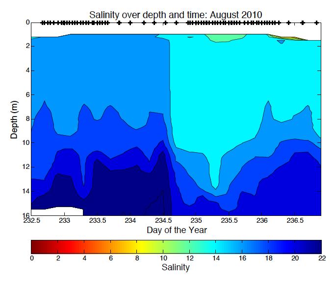
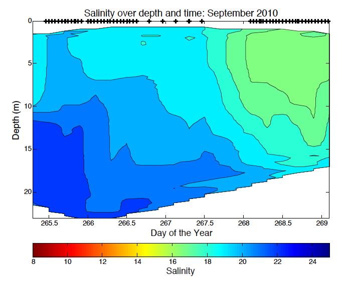
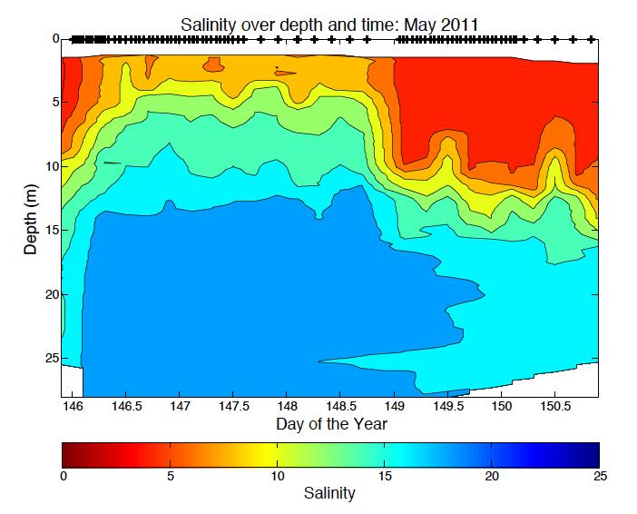
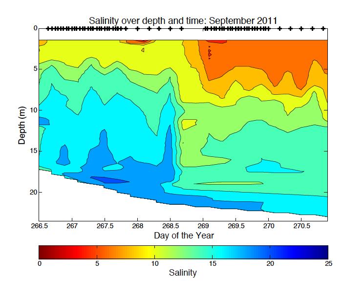
86 APPENDIX A: HYDROGRAPHIC DATA Appendix A.1. Salinity data for all cruises by day of year 78

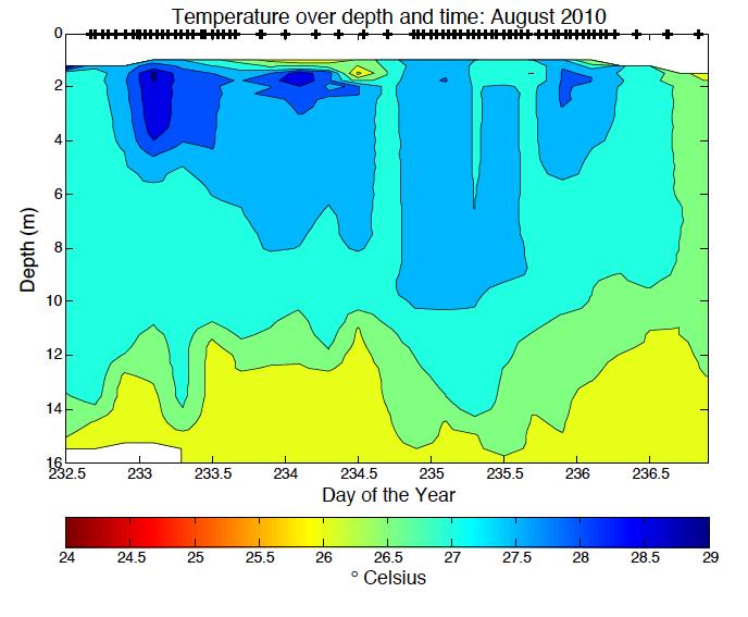
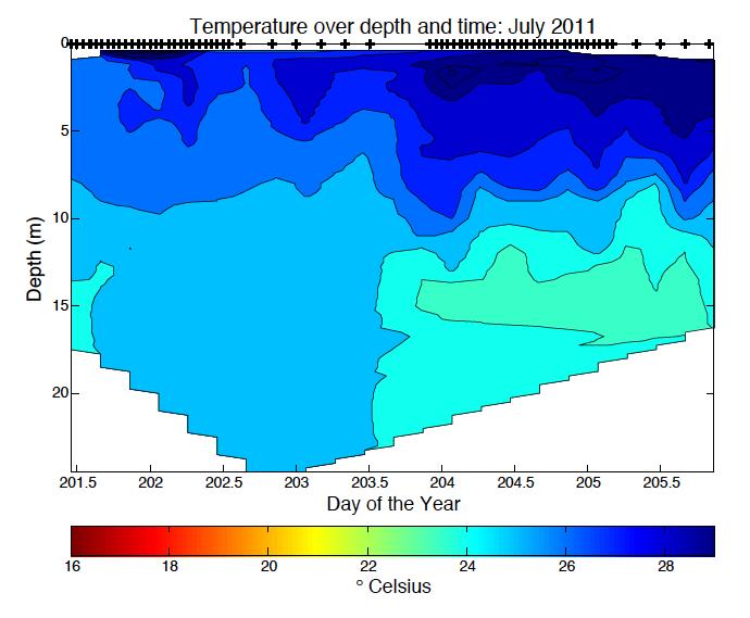
87 Appendix A.2. Temperature data for all cruises by day of year 79

88 Appendix A.3. Density data for all cruises by day of year. (Crosses represent CTD casts) 80

89 APPENDIX B: ACARTIA TONSA ABUNDANCE, VERTICAL DISTRIBUTION AND DIEL VERTICAL MIGRATION South Station North Station May 2010 August 2010 September

90 South Station North Station May 2011 July 2011 September 2011 Figure B.1. Acartia tonsa abundance separated by cruise and station 82

91 South Station North Station May 2011 July 2011 September 2011 Figure B.2. Acartia tonsa percent above and below the pycnocline separated by cruise and station APPENDIX C: SPECIES DIVERSITY 83

92 Species diversity and abundance varied with season and station. Acartia tonsa dominated samples regardless of station or season. The south station had higher species diversity than the north station during all cruises due the proximity to the mouth of the Bay with a greater influence from the Atlantic Ocean. There was greater species diversity in May and September in both 2010 and 2011 than in August 2010 and July Many species that were present in the spring cruises often disappeared in the summer cruises and again reappear in the fall samples. Eurytemora caroleaii, Labidocera sp., and Pseudodiaptomous sp. were the most common copepods aside from Acartia tonsa. Aside from copepod species, there were a few other species that were common during specific seasons and cruises. Podon sp. were often the second most dominant organism in spring and fall both years but less prevalent during the summer cruises. Barnacle nauplii and barnacle cyprid were consistently in high abundance during all seasons in 2010 but were less so in Fish eggs and fish larvae were more dominant in spring and summer cruises than in the fall. Phoronid larvae were not present in either spring cruise, but were found in higher numbers in summer and fall cruises both years. In August 2010 and July 2011, there were large numbers of Polychaetes present in samples. They were more prevalent at the north station but the numbers were not consistent with other seasons or years. 84

93 The pie charts representing species diversity do not include Acartia tonsa but all other species observed at the station and the relative abundance to each other (Appendix C1). May 2010 Ac#nula( Amphipod( Barnacle(Cyprid( Barnacle(Nauplii( Bosmina(Sp.( Centropages(Hamatus( Cumacean( Dinoflagellate(Spp.( Eurytemora(Affinis( Fish(Egg( Fish(Larvae( Flatworm(Larvae( Gammarid(Amphipod( Harpac#coid( Hydromedusae(Larvae( Labidocera(Aes#va( Mesocyclops(Spp.( Oithona( Paracalanus(Parvus( Paracalanus(spp.( Podon( Polychaete(Larvae( Pseudodiaptomus(Pelagicus( Shrimp(Spp.( Snail( Snail(Spp.( Tortanus(Spp.( UID1( 85

94 August 2010 Ac#nula( Barnacle(Cyprid( Barnacle(Nauplii( Bivalve(Larvae( Crab(Zoea( Eurytemora(Affinis( Fish(Egg( Fish(Larvae( Harpac#coid( Labidocera(Aes#va( Phoronid(Larvae( Podon( Polychaete(Larvae( Shrimp(Spp.( Snail( Tortanus(Spp.( September 2010 Ac#nula( Amphipod( Barnacle(Cyprid( Barnacle(Nauplii( Bivalve(Larvae( Bosmina( Chaetognath( Echinoderm(Larvae( Eurytemora(Affinis( Fish(Egg( Fish(Larvae( Formanifera( Harpac#coid( Hydromedusae( Labidocera(Aes#va( Larvacean( Oithona( Paracalanus(spp.( Phoronid(Larvae( Podon( Polychaete(Larvae( Polychaete(Pieces( Polychate(Pieces( Pseudevadne(Spp.( Pseudodiaptomus(Pelagicus( Shrimp(Spp.( Snail( Temora(Spp.( 86

95 May 2011 Ac#nula( Barnacle(cyprid( Barnacle(nauplii( Eurytemora( Fish(Egg( Fish(Larvae( Flatworm(Larvae( Harpac#coid( Isopod( Labidocera( Oithona( Oithona(spinirostris( Phoronid(Larvae( Podon( Polychaete(Larvae( Polychaete(Pieces( Pseudodiaptomous( Pseudovadne( Shrimp(spp( Snail( Temora( July 2011 Actinula Barnacle cyprid Bivalve Larvae Cyclopoid Fish Egg Fish Larvae Flatworm Larvae Gammarid amphipod Hydromedusae Labidocera Oithona Phoronid Larvae 87

96 September 2011 Ac#nula( Barnacle(cyprid( Barnacle(nauplii( Bivalve(Larvae( Bosmina( Chetagnath( Cyclopoid( Fish(Larvae( Fish(Lice( Flatworm(Larvae( Harpac#coid( Hydromedusae( Labidocera( Larvacean( Oithona( Paracalanus( Parvocalanus( Phoronid(Larvae( Podon( Polychaete(Pieces( Polychate(Larvae( Pseudo/evadne( Pseudodiaptomous( Shrimp(sp.( Snail( Unknown(worm(larvae( Appendix C.1. Species diversity by cruise 88