THE TEXAS RAPID ASSESSMENT METHOD (TXRAM)

Transcription

1 THE TEXAS RAPID ASSESSMENT METHOD (TXRAM) Wetlands and Streams Modules Version Final U.S. Army Corps of Engineers - Regulatory Division For use within the Fort Worth District in the State of Texas September 2015

2 The Texas Rapid Assessment Method (TXRAM) Wetlands and Streams Modules, Version 2.0 Final September 2015 Lead Agency: U.S. Army Corps of Engineers, Fort Worth District, Regulatory Division Lead Contractor: HDR Engineering, Inc. Supporting Contractors: Integrated Environmental Solutions, LLC Reviewing Agencies: U.S. Environmental Protection Agency U.S. Fish and Wildlife Service Texas Parks and Wildlife Department Texas Commission on Environmental Quality This report should be cited as: U.S. Army Corps of Engineers The Texas Rapid Assessment Method (TXRAM). Wetland and Streams Modules, Version 2.0. Final.

3 Additional Acknowledgement TXRAM Version 2.0 Based on Previously Prepared Version 1.0 U.S. Army Corps of Engineers The Texas Rapid Assessment Method (TXRAM). Wetland and Streams Modules, Version 1.0. Final Draft. Lead Agency: U.S. Army Corps of Engineers, Fort Worth District, Regulatory Division Lead Contractor: HDR Engineering, Inc. Supporting Contractors: Integrated Environmental Solutions, LLC SWCA Environmental Consultants Reviewing Agencies: U.S. Army Corps of Engineers, Tulsa District, Regulatory Division U.S. Environmental Protection Agency U.S. Fish and Wildlife Service Texas Parks and Wildlife Department Texas Commission on Environmental Quality Railroad Commission of Texas

4 Table of Contents FOREWORD... vi 1.0 INTRODUCTION Purpose Goal and Intended Use Geographic Scope Assessment Extent and Timing Based on Project Scope Other Technical Evaluations WETLANDS MODULE Background Information Key Terms Concepts and Assumptions Metrics Procedures Overview Ecoregion Wetland Type Wetland Assessment Area Field Assessment Preliminary Data Collection Utilizing Delineation Data General Instructions Office Review Calculating and Reviewing Scores Calculating TXRAM Scores Inferring Scores Quality Control Review Metric Evaluation Methods and Scoring Guidelines Landscape Aquatic Context Buffer Hydrology Water Source Hydroperiod Hydrologic Flow Soils Organic Matter Sedimentation Soil Modification Physical Structure Topographic Complexity Edge Complexity Physical Habitat Richness Biotic Structure Plant Strata Species Richness Non-native/Invasive Infestation Interspersion Strata Overlap...74 Texas Rapid Assessment Method i Table of Contents

5 Herbaceous Cover Vegetation Alterations References STREAMS MODULE Background Information Key Terms Concepts and Assumptions Metrics Procedures Overview Ecoregion Stream Type Assessment Reach Field Assessment Background information Utilizing Delineation Data General Instructions Office Review Calculating and Reviewing Scores Calculating TXRAM Scores Inferring Scores Quality Control Review Metric Evaluation Methods and Scoring Guidelines Channel Condition Floodplain Connectivity Bank Condition Sediment Deposition Buffer Condition Buffer In-stream Condition Substrate Composition In-stream Habitat Hydrologic Condition Flow Regime Channel Flow Status References Appendices Appendix A: Example Photographs Appendix B: Example Wetland Determination Data Forms Appendix C: TXRAM Wetland and Stream Data Sheets and Final Scoring Sheets Appendix D: Example Wetland Assessment Areas and Stream Assessment Reaches Texas Rapid Assessment Method ii Table of Contents

6 List of Figures Figure 1. Example of a stream with a narrow wetland fringe on banks which is assessed using the stream module... 2 Figure 2. Example of a stream with an abutting wetland and an adjacent wetland, where the stream is assessed using the stream module and the wetlands are assessed using the wetland module Figure 3. Example of a bed and banks that contain a wetland with minor braided channels where the area functions primarily as a wetland and is assessed using the wetland module Figure 4. Example of a wetland in a bed and banks where the area functions primarily as a wetland and is assessed using the wetland module Figure 5. TXRAM geographic scope within the USACE Fort Worth District in Texas Figure 6. TXRAM ecoregions based on EPA s Level III Ecoregions of Texas (Griffith et al. 2004) Figure 7. Flow chart for assessment extent and timing guidance based on project type Figure 8. Examples of WAA guidelines for complex situations Figure 9. Example of assessment extent on linear projects with typical ROW width Figure 10. Example of assessment extent on linear projects with non-typical ROW width Figure 11. Example of assessment extent on non-linear projects with known construction area Figure 12. Example of assessment extent on large non-linear projects without known construction area or for mitigation/conservation (e.g., potential mitigation bank) Figure 13. Flow chart for other technical evaluations Figure 14. Example of riverine wetland type (from Smith et al. 1995) Figure 15. Example of depressional wetland type (from Smith et al. 1995) Figure 16. Example of slope wetland type (from Smith et al. 1995) Figure 17. Example of lacustrine fringe wetland type (from Smith et al. 1995) Figure 18. Wetland type flow chart (adapted from Smith et al and Collins et al. 2008) Figure 19. Example of measuring aquatic context for a riverine wetland Figure 20. Example of measuring aquatic context for a slope wetland Figure 21. Example of measuring the buffer metric for a depressional wetland Figure 22. Example of measuring the buffer metric for a riverine wetland Figure 23. Example of measuring the buffer metric for a lacustrine fringe wetland Figure 24. Example of topographic complexity in a slope wetland Figure 25. Example of topographic complexity in a riverine wetland Figure 26. Example of topographic complexity in a lacustrine fringe wetland Figure 27. Examples of different scores for the topographic complexity metric Figure 28. Examples of vertical structure variability Figure 29. Examples of variability in the wetland boundary for use in qualitative evaluation of the edge complexity metric Figure 30. Examples of different degrees of interspersion for use in evaluating the interspersion metric Figure 31. Examples of the degree of strata overlap for wetlands with high and moderate overlap Figure 32. Examples of herbaceous species overlap and a dense litter layer in the herbaceous stratum with no other strata overlapping Figure 33. Example plan view of strata overlap scoring Figure 34. Example plan view of strata overlap scoring for WAA with multiple plant communities Figure 35. Example of bankfull bench situated below bankfull height Figure 36. Scoring classes and visual representations for the sediment deposition metric Figure 37. Example of measuring the primary riparian and secondary land-use buffers for an ephemeral stream Figure 38. Example of measuring the primary riparian and secondary land-use buffers for an intermittent stream Figure 39. Example of measuring the primary riparian and secondary land-use buffers for a perennial stream Figure 40. Scoring classes and visual representations for the substrate composition metric Texas Rapid Assessment Method iii Table of Contents

7 Figure 41. Example of scoring in-stream habitat metric with limited access to the SAR using 5- foot belt transects Figure 42. Example of scoring in-stream habitat metric with access throughout the SAR using 5- foot belt transects Figure 43. Example of riffle/pool sequence Figure 44. Scoring classes and visual representations for the flow regime metric Figure 45. Scoring classes and visual representations for the channel flow status metric Texas Rapid Assessment Method iv Table of Contents

8 List of Tables Table 1. Wetland and Stream Assessment Extent Guidelines... 7 Table 2. Wetland Functions and the Type of Ecosystem Process(es) Table 3. TXRAM Metrics Related to Ecosystem Processes Table 4. TXRAM Wetland Metrics by Core Element Table 5. TXRAM Wetland Types by Dominant Water Source and Hydrodynamics Table 6. Wetland Core Element Scoring Calculation Table 7. Example Calculation of Buffer Metric for Figure Table 8. Example Calculation of Buffer Metric for Figure Table 9. Example Calculation of Buffer Metric for Figure Table 10. Scoring Topographic Complexity Metric by Elevation Gradients and Percentage of Microtopography Table 11. Physical Habitat Types Potentially Present by Wetland Type Table 12. Scoring by Wetland Type for Physical Habitat Richness Metric Table 13. Example of Calculations for Species Richness Metric Table 14. Scoring Species Richness Metric in South Central Plains and East Central Texas Plains Ecoregions Table 15. Scoring Species Richness Metric in Southern Texas Plains, Edwards Plateau, Texas Blackland Prairies, and Cross Timbers Ecoregions Table 16. Scoring Species Richness Metric in High Plains, Southwestern Tablelands, and Central Great Plains Ecoregions Table 17. Example 1 of Calculations for Non-Native/Invasive Infestation Metric Table 18. Example 2 of Calculations for Non-Native/Invasive Infestation Metric Table 19. Example Calculation of Strata Overlap with Weighted Average Table 20. Scoring Strata Overlap Metric for Different Forms of Overlap Table 21. Stream Functions and the Type of Ecosystem Process(es) Table 22. TXRAM Metrics Related to Ecosystem Processes Table 23. TXRAM Stream Metrics by Core Element Table 24. TXRAM Stream Types Table 25. Stream Core Element Scoring Calculation Table 26. Primary and Secondary Buffer Distances by Stream Type Table 27. Example Calculation for Composite Left Bank Buffer Score for Figure Table 28. Example Calculation for Composite Right Bank Buffer Score for Figure Table 29. Example Calculation for Composite Left Bank Buffer Score for Figure Table 30. Example Calculation for Composite Right Bank Buffer Score for Figure Table 31. Example Calculation for Composite Left Bank Buffer Score for Figure Table 32. Example Calculation for Composite Right Bank Buffer Score for Figure Table 33. Scoring for Primary Buffer Types with Greater than 60% Tree Canopy Cover Table 34. Scoring for Primary Buffer Types with 30 60% Tree Canopy Cover Table 35. Scoring for Primary Buffer Types with less than 30% Tree Canopy Cover Table 36. Scoring for Secondary Buffer Types Table 37. Substrate Types, Sizes, and Reference Items Table 38. Example Calculation of In-stream Habitat Metric for Figure Table 39. Example Calculation of In-stream Habitat Metric for Figure Texas Rapid Assessment Method v Table of Contents

9 FOREWORD The Texas Rapid Assessment Method, (TXRAM) Version 1.0 was originally developed by the U.S. Army Corps of Engineers, Fort Worth District, Regulatory Division (USACE), and published in The USACE s team included Regulatory staff from the Fort Worth and Tulsa Districts, and experienced delineators and permitting personnel from three private consulting firms, in addition to field review and input from cooperating state and federal agency staff. The methodology was developed in approximately one year. The objective of the effort was to develop a tool for evaluating stream and wetland conditions that was rapid and repeatable in order to enhance the consistency of the USACE s permit decision-making processes as well as project proponents and applicants in planning, alternative evaluations, impact assessments, and mitigation plan development. In March 2011, the USACE issued a Public Notice announcing the availability of the Final Draft of TXRAM Version 1.0 (dated October 2010) via the USACE s website. Due to the broad scope of TXRAM, including the application in aquatic habitat types throughout the Fort Worth and Tulsa Districts, the USACE encouraged practitioners to utilize it throughout the region and accepted written comments for one year. The USACE received approximately 131 separate comments on the components and application of TXRAM. While Version 1.0 achieved the USACE s objectives for the evaluation tool, additional use and comments highlighted areas where the method could be improved. In 2014, the USACE initiated the finalization of the TXRAM with the goal of making revisions to parts of the method where concerns had been identified, an effort that resulted in this manual, TXRAM Version 2.0. The process for the development of Version 2.0 included consideration of comments received during the one-year review of Version 1.0; input from practitioners with extensive field experience using TXRAM; input from USACE and other resource agency staff that evaluate/review TXRAM results; and multiple field review efforts to refine revised metrics and weighting of core elements. The USACE Team s objectives in the development of Version 2.0 include: Maintain high scoring for habitat types with heterogeneous, diverse conditions, while improving quantification of condition elements for large, high-quality uniform habitats, such as contiguous bottomland hardwood forested wetlands. Retain appropriately higher level scoring for relatively rare habitat features and adjust scoring approach for common metrics (e.g., edge complexity), while maintaining sensitivity to measure when these features occur and influence aquatic habitat function. Enhance measurement and sensitivity of metrics related to hydrology and aquatic habitat availability and condition. Refine the measurement and evaluation of stream buffers to balance both the influence on adjacent habitat and the function of buffers to maintain stream condition, with recognition that the USACE s jurisdiction is over waters of the U.S. Evaluate relationship of biotic assessments to TXRAM and provide practitioners with information regarding when other evaluation methods may be required. Texas Rapid Assessment Method vi Foreword

10 During the revision process, the USACE s team made substantial changes to several metrics as well as weighting of core metrics (see summary below). Conversely, after careful evaluation of potential modifications, several metrics were kept the same or nearly so. Also, many of the metric scoring narratives for both wetlands and streams were enhanced to improve effectiveness and clarity. The USACE appreciates the input from commenters to previous TXRAM Version 1.0 and staffs of cooperating agencies for providing useful input to the revision process. The USACE Team considers the TXRAM Version 2.0 manual has achieved the objectives as well as the overall goal, which was to improve the tool s usefulness for USACE, project planners, and applicants in evaluating, protecting, and enhancing the important aquatic resources within our region. Summary of significant changes: Version 1.0 Version 2.0 General Includes general statement on other analyses being required by USACE on project-specific basis, The addition of section 1.5 provides a framework and flow chart for determining when biotic but did not address situations when biotic assessments and other technical evaluation assessment or other data analysis is required. techniques may be required for the USACE s Scoring narratives, scoring sheets, and representative photographs included. Wetlands Module Core elements weighted equally (20% of total score) Edge complexity uses plan view variability and edge-to-area ratio for scoring Stream Module Core elements weighted equally (25% of total score) Riparian buffers on each side of channel extend 100 feet for perennial, 50 feet for intermittent, and 25 feet for ephemeral streams Substrate composition evaluates bedrock as uniform and large woody debris/leaf packs not considered In-stream habitat evaluated with visual transects for presence of 10 habitat types Regulatory decision-making process. Many of the scoring narratives and exhibits were revised to improve clarity, as well as additional representative photographs. Expanded scoring sheets for wetlands and streams to allow scoring of existing and multiple future condition / alternatives for side-by-side comparison. Weight of hydrology core element increased to 30%, weight of landscape and soils decreased to 15%, physical and biotic structure stay at 20% Edge complexity revised to remove edge-to-area ratio and now considers surrounding habitat with hydrologic setting and vertical structure complexity Weight of channel condition core element increased to 30%, weight of buffer condition decreased to 20%, in-stream and hydrologic condition stayed at 25% Total buffer for all stream types extends to 150 feet, with primary and secondary areas weighted and evaluated separately (widths vary by type) Scoring refined for additional sensitivity on lower scores with complete category of human/domestic animal use. Substrate composition includes evaluation of large woody debris/leaf packs, differentiates between uniform and fractured bedrock, and clarifies scoring narratives with some revised percentages In-stream habitat evaluated with a defined belt width of transects, along with addition of habitat types bedrock with interstitial space, canopy cover, and natural step pools, as well as scoring using estimation of percent cover for certain habitat types Texas Rapid Assessment Method vii Foreword

11 1.0 INTRODUCTION 1.1 Purpose The Fort Worth District of the U.S. Army Corps of Engineers (USACE), Regulatory Division, has developed this manual to provide a rapid assessment method for evaluating the ecological condition of jurisdictional wetlands and streams. This manual contains two separate modules one for wetlands and one for streams which each describe the intended use, scope, background, procedures, and guidelines for the Texas Rapid Assessment Method (TXRAM). The output from TXRAM will be used for calculating adverse impacts and compensatory mitigation associated with USACE authorized activities under Section 404 of the Clean Water Act and Section 10 of the Rivers and Harbors Act of The appropriate use of TXRAM will provide consistent methods for wetland and stream assessment and will support the integrity of data collection and comparison. 1.2 Goal and Intended Use The goal of TXRAM is to provide a rapid, repeatable, and field-based method that generates a single overall score of wetland or stream integrity and health. As such, TXRAM does not focus on specific ecologic functions or societal values provided by wetlands and streams. Although TXRAM will be sufficient in most regulatory situations, the USACE may request additional assessment of specific functions since TXRAM is not an intensive, quantitative functional assessment. The USACE will decide on a case-by-case basis, commensurate with the level and/or type of impacts, whether more detailed information and analysis is needed to meet regulatory requirements. TXRAM is intended to provide information for the evaluation of the current and potential future in the case of restoration or mitigation efforts ecological conditions of wetlands and streams that meet the definition of a water of the U.S. in place at the time of the evaluation; however, it is not intended to be used to evaluate the jurisdictional status of a stream or wetland to determine if it is a water of the U.S. The evaluation of the jurisdictional limits and status of a stream, wetland, or other aquatic sites that are potentially waters of the U.S. is to be conducted using the appropriate USACE delineation method and guidance for jurisdictional determinations published jointly for that purpose by USACE and the U.S. Environmental Protection Agency (USEPA) in place at that time. Several metrics for both streams and wetlands may require the assessment of landscape conditions beyond the limits of the waters of the U.S. to determine those factors influencing the existing and future condition of the aquatic resource. TXRAM can be conducted utilizing both on-site and/or remote sensory data (in circumstances where access is limited or unavailable). The recommendation to perform TXRAM in support of potential regulatory actions shall not be construed as a determination or extension of jurisdictional authority as granted under the Clean Water Act, and does not grant the TXRAM evaluator the authority to access property without permission of the landowner. Within the USACE Regulatory Program, TXRAM may be used to assess potential wetland or stream impacts, including the comparison of project alternatives. TXRAM may also be used in association with monitoring requirements to track the changes in actual wetland or stream conditions over time. In the context of mitigation activities, TXRAM may be used to evaluate the future, proposed ecological conditions of a wetland or stream that meets the definition of a water of the U.S., but there may be other evaluations, information, and guidelines required (see Texas Rapid Assessment Method 1 Introduction

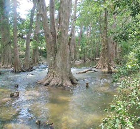
12 section 1.5). Further applications or uses of TXRAM may be desirable or feasible, but should be verified by the USACE prior to implementation. TXRAM scores are generally intended to be interpreted and compared between resources of the same type, and the comparison of scores between different wetland or stream types may not provide an accurate depiction of condition and functions the aquatic sites provide in the landscape or watershed setting. Furthermore, the development and use of TXRAM assumes that scores for wetlands and streams should be interpreted and compared within the same ecoregion in order to accurately reflect differences in condition. TXRAM includes some considerations for different ecoregions in metric scoring, but this is not intended to normalize the scores for every ecoregion. Thus, the same TXRAM score for wetlands or streams in different ecoregions may not reflect the same condition; nor does a lower score for a wetland or stream in a different ecoregion mean that it necessarily represents a lower level of function the aquatic site provides within its watershed and landscape setting. Therefore, TXRAM scores should generally be interpreted for wetlands or streams of the same type and ecoregion, including the use of a reference standard of highest condition (which may not reach the theoretical maximum score). However, since compensatory mitigation evaluations are generally based on the assessment of conditions and functions aquatic sites provide within limited watershed and ecoregion areas as outlined in the 2008 Final Rule on Compensatory Mitigation for Losses of Aquatic Resources, the differences between resource types and ecoregions is not considered to be a concern from a regulatory process perspective. TXRAM contains a module for wetlands and a module for streams, but does not apply to lentic open waters (e.g., lakes and ponds), vegetated shallows, mudflats, or other aquatic features. The applicable module for an aquatic feature should be based on regulatory definitions, the delineation, and how it currently functions. For example, a stream with a narrow fringe of wetland vegetation on the banks should be assessed using the stream module. However, the wetland module should be used to assess a distinct wetland abutting a stream channel or a bed and banks that contain a wetland with minor braided channels where the area functions primarily as a wetland. Figures 1 4 illustrate the applicable model for some general situations. Areas that have been modified by disturbance or stress (e.g., channelization) may be in a state of transition from one type of aquatic feature to another based on channel morphology, sediment loads, hydrology/hydraulics, and other factors. In complex or atypical situations where the applicable module is unclear, the user should coordinate with the USACE for assistance or exercise professional judgment. The USACE has the final authority to decide which module applies to an aquatic feature. Figure 1. Example of a stream with a narrow wetland fringe on banks which is assessed using the stream module. Texas Rapid Assessment Method 2 Introduction

13 Figure 2. Example of a stream with an abutting wetland and an adjacent wetland, where the stream is assessed using the stream module and the wetlands are assessed using the wetland module. Figure 3. Example of a bed and banks that contain a wetland with minor braided channels where the area functions primarily as a wetland and is assessed using the wetland module. Figure 4. Example of a wetland in a bed and banks where the area functions primarily as a wetland and is assessed using the wetland module. A field review of TXRAM Version 2.0 was performed May 11 14, June 9 11, and August 20 21, 2015, by the USACE, their contractors, and reviewing agencies in order to evaluate and calibrate both the wetlands and streams modules. The field review consisted of applying TXRAM to actual wetlands and streams in different ecoregions that occur in the Fort Worth District within Texas. Information obtained during the field review has been incorporated into this version of TXRAM. Texas Rapid Assessment Method 3 Introduction

14 1.3 Geographic Scope The geographic scope of this version of TXRAM is limited to the USACE Fort Worth District located within Texas (Figure 5). Although TXRAM may be generally applicable outside this geographic scope, it has not been tested and field calibrated in other areas. As such, any results should be considered in light of this limitation. TXRAM utilizes the U.S. Environmental Protection Agency 2004 Level III Ecoregions of Texas (Griffith et al. 2004). The ecoregions included within the geographic scope of TXRAM include the South Central Plains (also known as the Pineywoods), East Central Texas Plains (also known as the Post Oak Savannah or Claypan Area), Texas Blackland Prairies, Cross Timbers, Southern Texas Plains, Edwards Plateau, Central Great Plains, Southwestern Tablelands (collectively with the Central Great Plains also known as the Rolling Plains), and High Plains (Figure 6). Figure 5. TXRAM geographic scope within the USACE Fort Worth District in Texas. Texas Rapid Assessment Method 4 Introduction

15 Figure 6. TXRAM ecoregions based on EPA s Level III Ecoregions of Texas (Griffith et al. 2004). Texas Rapid Assessment Method 5 Introduction

16 1.4 Assessment Extent and Timing Based on Project Scope The implementation of TXRAM may vary in the extent and timing of assessment for different types of projects. For example, the assessment may be performed during or after a delineation of waters of the U.S. Figure 7 provides guidance and options for how and when to perform an assessment based on the type of project proposed. Users may exercise professional judgment when planning the timing of the assessment in conjunction with other project activities, and may also coordinate with the USACE for additional guidance. Figure 7. Flow chart for assessment extent and timing guidance based on project type. In wetlands, a wetland assessment area (WAA) is evaluated to determine a score of ecological condition. In streams, a stream assessment reach (SAR) is evaluated to determine a score of ecological condition. The WAA and SAR are defined as the area where all measures and metrics are observed and scored in order to calculate the overall TXRAM score. The effective use of TXRAM requires consistency and repeatability among users when determining the WAA and SAR in order to allow the results of TXRAM to be productive and informative as to the condition of the evaluated wetland(s) and/or stream(s). A WAA or SAR should always be representative of the wetland or stream that is being assessed, whether it is a small wetland, large mosaic of wetlands, small ephemeral stream, or large perennial river. The wetland and stream assessment extent guidelines in Table 1 are intended to assist users in consistently setting the WAA and SAR boundary. Texas Rapid Assessment Method 6 Introduction

17 Table 1. Wetland and Stream Assessment Extent Guidelines Wetland Assessment Area Guidelines (Adapted from Mack 2001): Setting the WAA is a critical step in the TXRAM procedures and can influence the overall score. Since determining the boundary of the WAA can potentially be complex, the guidelines below are intended to provide information for accurately and consistently setting the area to be assessed. Based on scientific literature, the guidelines focus on encompassing the entire wetland area with uniform hydrologic processes in a single WAA. Set the WAA using the steps and guidelines below. Identify the wetland area of interest (impacted areas, mitigation areas, etc.). Utilize aerial photography to evaluate the consistency of light/color signatures in the wetland. Identify the location(s) where there is physical evidence of a substantial change in the hydrology of the wetland. Hydrology is the main criterion that should be used to determine the boundary of the WAA. In the absence of a change in hydrology, the WAA should encompass the entire wetland and follow the wetland boundary. Boundaries of the WAA between contiguous or connected wetlands should be established where the volume, flow, source, or velocity of water moving through the wetland distinctly changes. These changes could be natural (topographic, wildlife activities, debris, etc.) or human-made (berms/dikes, ponds, weirs, infrastructure, etc.). Except as described below, the WAA boundary should encompass all wetland areas with uniform hydrologic processes. This means that all contiguous wetland areas of the same wetland type (see section for discussion) that have a high degree of hydrologic interaction should be included in the same WAA, regardless of the vegetation community. In addition to hydrology, the boundary of the WAA should also be established where conditions vary in a wetland due to disturbance or stress. For example, a single riverine wetland that is partially mature, diverse forest and partially early successional, low diversity forest (due to past logging) would require separate WAAs for the two different areas (Figure 8A) which vary by past stressors (i.e., vegetation alteration). Justification for splitting a wetland area with uniform hydrologic processes into multiple WAAs should be described and documented in the TXRAM data sheet and final scoring sheet. As described above, it is not necessary to establish separate WAAs in wetlands that are a mosaic of several different vegetation communities if the area has largely uniform hydrologic processes and a high degree of hydrologic interaction. For example, a 4-acre riverine wetland with both forested and emergent communities should have a single WAA (Figure 8B), and a 20-acre riverine wetland with forested, emergent, and scrub/shrub vegetation communities should have a single WAA (Figure 8C). Artificial boundaries (e.g., property lines, county lines, city limits, roads, railroads, pipelines, etc.) should not be used for the WAA boundary unless they coincide with a hydrologic change or a change in condition due to disturbance or stress as described above. However, as in the case of linear projects, if property access is only available for a portion of the wetland, the WAA may be set accordingly and described in the TXRAM data sheet and final scoring sheet. Some wetlands occur in conjunction with open water areas. The following guidelines should be utilized to determine the WAA for wetlands contiguous to open water. 1. If the open water area is 20 acres or less, then the WAA should include all wetlands of the same type that are contiguous to that area of open water. 2. If the open water area is greater than 20 acres, then separate WAAs are required for each separate wetland contiguous to the open water area. 3. A separate WAA is required for wetlands that are contiguous to an open water area and a stream but whose hydrology is predominantly influenced by the stream channel (i.e., a different wetland type than other wetlands contiguous to the open water area). Separate WAAs should be established for two or more wetlands directly abutting a channel if: 1. The wetlands are located on opposite sides of a channel that is greater than 100 feet in width on average, 2. The wetlands are separated by a non-wetland corridor (along the channel) greater than 100 feet, or 3. The wetlands are separated by a wetland corridor along the channel that is less than 50 feet in width (including the channel) at the widest point for greater than 100 feet in length. The WAA can be adjusted in the field during or after the delineation using the guidelines above. Texas Rapid Assessment Method 7 Introduction

18 Table 1 (continued). Wetland and Stream Assessment Extent Guidelines Stream Assessment Reach Guidelines: Identify the stream area (river, stream, channel, etc.) of interest (impacted areas, mitigation areas, etc.) The stream areas of interest may then further be divided into multiple Stream Assessment Reaches (SAR) which are established by distinct changes in any of the following parameters: 1. Channel Condition: both current and historic which can be visually assessed by identifying several geomorphologic indicators (channel incision, access to floodplain, channel widening, channel deposition features, rooting depth compared to streambed elevation, stream bank vegetation protection, and stream bank erosion). 2. Riparian Buffer Condition: the area surrounding a stream extending from each bank that influences the effects of stressors and provides potential benefits in relation to stream condition. Changes in the riparian buffer and vegetation community surrounding the stream necessitate separate SARs. For example, the riparian buffer along an intermittent stream may consist of an 80-foot band of forested area, but then the stream flows into an area that is farmed, and the band of riparian forest narrows to 20 feet. As a result, the stream would have one SAR in the portion of the stream with an 80-foot band of riparian forest and a separate SAR in the area with the 20-foot band of riparian forest. Similarly, if a stream is located in a wooded area and then flows into a pasture with no trees, then a SAR should be located in the wooded community, and a separate SAR should be located in the pasture community. 3. In-Stream Condition: the habitat and substrate suitable for the effective colonization or use by fish, amphibians, and/or macroinvertebrates. A distinct change in the in-stream habitat should require the separation of a SAR. For example, a stream dominated by large woody debris with cobbles that transitions downstream to a portion free of snags with bed composed of silt and clay would require separate SARs for each section of the stream. 4. Stream Type/Hydrologic Condition: the stream type as categorized as ephemeral, intermittent, or perennial. A change from one stream type to another would require a separate SAR. Additionally, a change in channel flow could also warrant a separate SAR. For example, separate SARs would be required where an intermittent stream with water reaching from bank to bank changes to a predominantly dry ephemeral stream. Channel alteration (i.e., direct impacts to the stream channel from human-made sources) should also be used to distinguish SARs. These human-made sources may include, but are not limited to, channelizing the stream, bridges and/or culverts, riprap along the stream bank, stream bank stabilization materials (e.g., gabion baskets, concrete blocks, concrete walls, etc.), human-made embankments on the stream bank, constrictions to the stream (e.g., development, infrastructure, etc.), and livestock impacts. The natural stream and the altered stream channel would have separate SARs. Stream length should be utilized to establish a SAR. Project areas that have more than ¼ mile (1,320 linear feet) of one channel within the project area boundary should be separated into multiple SARs, at least one SAR for every ¼ mile of channel. For example, a 1-mile channel in a project area that has a consistent channel condition, riparian buffer condition, in-stream condition, and no channel alteration should have at least four separate SARs to be reviewed and documented. Separate SARs for every ¼ mile of channel will ensure that conditions for long stream segments are adequately assessed to capture the representative variability. Instructions for inferring scores on a stream with multiple SARs that have very similar characteristics are found in section Texas Rapid Assessment Method 8 Introduction

19 Figure 8. Examples of WAA guidelines for complex situations. In many cases, the first step in determining the WAA or SAR is to determine the type of project proposed. The following discussion on determining the type of project is meant to help users streamline the assessment based on the extent and timing needed for a specific project. The user must determine if the proposed project will: 1) result in the placement of fill material into waters of the U.S., or 2) result in the mitigation (e.g., restoration, establishment, enhancement, or preservation) for impacts to waters of the U.S. The assessment extent and timing flow chart (Figure 7) illustrates potential steps that will assist in determining the WAA and/or SAR for different types of proposed projects. The discussion and flow chart for determining assessment extent and timing based on project type may not fit every project or situation, so professional judgment and USACE coordination may be necessary when determining the extent and timing of the assessment. The USACE has the authority to make the final determination on the location of the WAAs and/or SARs within the proposed project area. Figures 9 12 provide examples to illustrate the WAA and SAR boundaries for different project types discussed below and based on the guidelines in Table 1. The SAR boundaries in Figures 9 12 have been drawn along the channel and not encompassing the riparian area for simplifying the depiction. For those projects that will result in the placement of fill material into waters of the U.S., the assessment extent will differ between linear and non-linear project types (Figure 7). Linear projects are those projects constructed for the purpose of getting people, goods, or services from a point of origin to a terminal point and typically include roadways, railroads, pipelines, and transmission lines. Non-linear projects are all other types of projects that typically cover an area of land. Linear projects within the Fort Worth District typically have a right-of-way (ROW) that is approximately 200 feet or less in width. Where the ROW is typical, a single WAA and/or SAR may be located at each individual crossing location (Figures 9A, 9B, and 9C), or the crossing may require the use of multiple WAAs and/or SARs based on the guidelines in Table 1 (Figures 9D and 9E). In situations where the ROW for a linear project exceeds 200 feet (i.e., a nontypical ROW), a single WAA and/or SAR may be located at each individual crossing location (Figure 10A), or the crossing may require the use of multiple WAAs and/or SARs (Figures 10B and 10C). The location of these WAAs and/or SARs should be determined in the field during the delineation of waters of the U.S. using the guidelines set forth in Table 1. Texas Rapid Assessment Method 9 Introduction

20 Figure 9. Example of assessment extent on linear projects with typical ROW width. Figure 10. Example of assessment extent on linear projects with non-typical ROW width. Texas Rapid Assessment Method 10 Introduction

21 Non-linear projects may be any size, including large commercial developments or small outfall structures. The assessment extent will also differ between non-linear projects where the construction/impact area is known as opposed to not known prior to the assessment (Figure 7). If the construction/impact area for the project is known prior to the assessment, then a delineation of waters of the U.S. should be performed within the construction/impact area boundary. The WAAs and/or SARs for TXRAM should then be located in the waters of the U.S. that would be impacted by the proposed project (Figure 11). The location of these WAAs and/or SARs may be determined during or after the delineation of waters of the U.S. using the guidelines set forth in Table 1. TXRAM should then be completed within each WAA and/or SAR (as described in the wetland module and/or stream module) in conjunction with the delineation of waters of the U.S. or in a subsequent field visit (Figure 7). Figure 11. Example of assessment extent on non-linear projects with known construction area. Non-linear projects in which the construction/impact area is not known prior to the assessment may utilize two different options to determine the WAAs and/or SARs (Figure 7). The first option for determining the WAAs and/or SARs for these non-linear projects is to complete a preliminary Texas Rapid Assessment Method 11 Introduction

22 in-office photo-interpretation of the project area. This includes identifying all potential waters of the U.S. as viewed on recent aerial photography and other available information (e.g., USGS maps, soils surveys, Geographic Information System [GIS] layers) and then identifying WAAs and/or SARs based on those photo-interpreted areas (Figure 12). The WAAs should be located within the photo-interpreted wetland boundaries, and the SARs should be located along the photo-interpreted stream channels and associated riparian buffers based on the guidelines set forth in Table 1. TXRAM should then be completed within each WAA and/or SAR (as described in the wetland module and/or stream module) in conjunction with the delineation of waters of the U.S. (Figure 7).The second option for these non-linear projects is to determine the WAAs and/or SARs during or after the delineation of waters of the U.S. within the project area (Figure 12). The WAAs and/or SARs should be located in the waters of the U.S. identified during the delineation based on the guidelines set forth in Table 1. TXRAM should then be completed within each WAA and/or SAR (as described in the wetland module and/or stream module) in conjunction with the delineation of waters of the U.S. or in a subsequent field visit (Figure 7). Figure 12. Example of assessment extent on large non-linear projects without known construction area or for mitigation/conservation (e.g., potential mitigation bank). Texas Rapid Assessment Method 12 Introduction

23 For those projects that will result in the mitigation for impacts to waters of the U.S., the location of the WAAs and/or SARs should be determined after completing a delineation of waters of the U.S. within the project area (Figure 7). The WAAs and/or SARs should be located in the waters of the U.S. identified during the delineation based on the guidelines set forth in Table 1. TXRAM should then be completed within each WAA and/or SAR (as described in the wetland module and/or stream module) in a subsequent field visit (Figure 12). Another option is to submit the delineation of waters of the U.S. to the USACE for verification and a jurisdictional determination prior to determining the WAAs and SARs in order to assure TXRAM is completed on all waters of the U.S. Finally, for all project types, the WAA and SAR boundaries may be adjusted in the field in accordance with the guidelines in Table 1. In addition, the locations of the WAAs and/or SARs for large and/or complex wetlands and streams may need to be verified by the USACE prior to the completion of the TXRAM field assessment. Coordination with the USACE on the locations of the WAAs and/or SARs is not a requirement but a recommendation for the completion of TXRAM in an efficient and timely manner (Figure 7). In particular, USACE coordination is recommended for large projects such as individual permit applications and potential mitigation banks. The USACE has the authority to make the final determination on the location of the WAAs and/or SARs within the proposed project area. 1.5 Other Technical Evaluations TXRAM is intended to serve as a rapid evaluation tool useful in planning and impact assessments for those USACE Regulatory Program evaluations suitable for Nationwide Permit (NWP) authorizations and Individual Permits without significant adverse environmental impacts. A relatively small percentage of the Section 404 actions will require a variety of more comprehensive or resource-specific evaluation techniques. Supplemental techniques and other technical evaluations of aquatic resources may be required for a subset of USACE Regulatory Program actions, as shown in the flow chart below (Figure 13). Note that this does not preclude the need for evaluations of cultural resources, endangered species, and other factors as part of public interest review for regulatory actions. Figure 13. Flow chart for other technical evaluations Other evaluations may include, but are not limited to, Rosgen stream classification, habitat modeling, biotic sampling, fluvial geomorphic classification, natural stream channel design techniques, water quality investigations, wildlife habitat studies, hydrologic/hydraulic modeling, Texas Rapid Assessment Method 13 Introduction

24 or others. Additionally, some actions such as proposed mitigation activities may require other evaluations such as those listed above commensurate with the proposed activities and the need to quantify the proposed influence on ecological conditions/functions of aquatic resources. Other technical evaluations may be used in the USACE Regulatory Program in addition to TXRAM but are not intended to replace, or be incorporated into, TXRAM scores. Texas Rapid Assessment Method 14 Introduction

25 2.0 WETLANDS MODULE The TXRAM Wetlands Module is intended to aid in assessing the condition of the different wetland types found in Texas throughout the USACE Fort Worth District. The module contains sections on background information, procedures, and guidelines for evaluating and scoring a series of metrics to arrive at an overall score of wetland integrity. 2.1 Background Information This section will provide background on the use of TXRAM for wetlands including the key terms, concepts and assumptions, and the metrics Key Terms To ensure consistency in the use of key terms, it is necessary to define the following assessment terms. Wetland Assessment Area (WAA): the portion of a wetland that is evaluated and scored using TXRAM. This encompasses the entire wetland area with uniform hydrologic processes; however, multiple wetland assessment areas may be needed for wetlands with varying conditions related to disturbance or stress. Additional information on how the assessment area is set can be found in section 1.4. Buffer: the area surrounding a wetland that influences the effects of stressors and disturbance (that originate outside the wetland) on wetland condition. Condition: the quality, integrity, or health of a wetland determined by the interactions of hydrologic, biologic, chemical, and physical processes. Condition is also the ability of a wetland to support and maintain its complexity and capacity for self-organization. Disturbance: a natural event that affects the processes and subsequently the condition of a wetland. Elevation gradients: changes in height that affect the level of saturation/inundation or the path of water flow. Elevation gradients typically have greater than 6 inches of difference with a corresponding change in saturation/inundation, soil condition, and/or vegetation. Function: a process or attribute (physical, chemical, or biological) that is performed by a wetland that supports its integrity and occurs whether or not it is deemed valuable by society. Metric: a characteristic or indicator of wetland condition that is evaluated and scored in the rapid assessment and which is grouped with other metrics into a category of landscape, hydrology, soils, physical structure, or biotic structure. Micro-topography: both micro-highs and micro-lows that are generally interspersed, local in extent, and typically have 3 6 inches of elevation difference from the surrounding area with a corresponding change in saturation/inundation, soil condition, and/or vegetation. Texas Rapid Assessment Method 15 Wetlands Module

26 Physical habitat types: different structural surfaces and features that support the living requirements of flora and fauna (e.g., un-vegetated pools, thick herbaceous cover, standing snags). Plant zones: different associations of plants within a community that are organized along elevation or hydrologic gradients over the surface of a wetland. Process: a series of steps that occur to move or change a particular resource (e.g., water, energy, nutrients). Stress/Stressor: a human activity or human-caused event which affects the processes and subsequently the condition of a wetland. Value (not related to soil color): the worth or desirability assigned to something (e.g., a wetland attribute) by society (i.e., humans). Other terms used in this manual which are not defined here (such as regulatory and wetland delineation terms) will follow the definitions in the references below. Brinson, M.M A Hydrogeomorphic Classification for Wetlands. Technical Report WRP-DE-4, U.S. Army Engineer Waterways Experiment Station, Vicksburg, MS. Code of Federal Regulations, Title 33, Part 328, Section ( ) Definitions. Environmental Laboratory Corps of Engineers Wetlands Delineation Manual. Technical Report Y-87-1, U.S. Army Engineer Waterways Experiment Station, Vicksburg, MS. USACE Regional Supplement to the Corps of Engineers Wetland Delineation Manual: Arid West Region (Version 2.0). Ed. J.S. Wakeley, R.W. Lichvar, and C.V. Noble. ERDC/EL TR Vicksburg, MS: U.S. Army Engineer Research and Development Center. USACE. 2010a. Regional Supplement to the Corps of Engineers Wetland Delineation Manual: Atlantic and Gulf Coastal Plain Region (Version 2.0). Ed. J.S. Wakeley, R.W. Lichvar, and C.V. Noble. ERDC/EL TR Vicksburg, MS: U.S. Army Engineer Research and Development Center. USACE. 2010b. Regional Supplement to the Corps of Engineers Wetland Delineation Manual: Great Plains Region (Version 2.0). Ed. J.S. Wakeley, R.W. Lichvar, and C.V. Noble. ERDC/EL TR Vicksburg, MS: U.S. Army Engineer Research and Development Center Concepts and Assumptions Several concepts and assumptions were followed and made in the development of TXRAM for wetlands regarding wetland structure and function. These concepts and assumptions affect the ways in which the metrics were developed and scored as well as the application of the TXRAM output. The concepts and assumptions are described below. Texas Rapid Assessment Method 16 Wetlands Module

27 As discussed previously, TXRAM allows the relatively rapid, qualitative measurement of the overall condition (i.e., integrity) of a wetland as opposed to quantitatively measuring specific ecologic functions (processes) or societal values provided by a wetland. An assessment of condition provides a general evaluation and integrated score of overall ecosystem health (based on physical and biological structural attributes) from which the relative functional capacity of a wetland is inferred (Stein et al. 2009). The measurement of condition fits with the goal of TXRAM being a rapid and repeatable method that outputs a single score. Assessing condition avoids the difficulty of quantifying multiple functions of a wetland and the issues associated with combining multiple functions into a single score (Fennessy et al. 2007). By measuring the position at which a wetland lies on the continuum of integrity, TXRAM assesses the integration of physical, chemical, and biological processes that maintain an ecosystem over time. Thus the assessment of wetland condition with TXRAM meets the requirements of the USACE Regulatory Program for an assessment method for the majority of authorized activities under Section 404 of the Clean Water Act. However, the potential impacts associated with some proposed projects may require that additional, more quantitative methods be applied. The TXRAM Wetlands Module was developed based on the concept that the condition of a wetland is determined by interactions among internal and external hydrological, biological, chemical, and physical processes. Climate and geology are the overarching factors that control natural abiotic and biotic processes in a wetland. Climate and geology also directly influence the hydrology of a wetland, which is the most important determinant of the establishment and maintenance of wetland processes (Mitsch and Gosselink 2000). The hydrology in turn determines and modifies the physiochemical environment of a wetland (e.g., oxygen availability, nutrient availability, sediment input). The physiochemical environment then influences the biota (e.g., vegetation, animals, and microbes) that inhabit a wetland. Feedback from biota can modify the physiochemical environment and hydrology of a wetland through their influence on both abiotic and biotic processes (e.g., microbes transform nutrients, plants trap sediment, and animals harvest vegetation). The physiochemical environment may also directly modify the hydrology of a wetland by changing the topography or flow of water (e.g., through accumulation of sediment). TXRAM assumes the condition of a wetland is influenced by the quantity and quality of water and sediment either generated on-site or exchanged between the site and the immediate surroundings (Collins et al. 2008). The water and sediment resources affecting a wetland are ultimately controlled by climate, geology, and land use. Geology and climate control natural disturbances which affect wetlands, whereas land use determines human stressors impacting a wetland. Biological components of a wetland (primarily vegetation) help mediate the influence of geology, climate, and land use on the quantity and quality of water and sediment. Stressors and disturbance typically originate outside the wetland (in the surrounding landscape), but buffers around the wetland tend to reduce the effects of these influences on wetland condition (e.g., capture nutrients, dissipate flow, reduce sediment deposition). The assessment of a wetland using TXRAM assumes that condition varies along a gradient based on stressors, and the condition that results can be evaluated based on a set of visible field metrics (Sutula et al. 2006). TXRAM also assumes that the condition of a wetland improves as structural complexity increases (Collins et al. 2008). Thus the scoring of wetlands using TXRAM assumes that the value of a wetland is determined by the ecological services provided to society, and the diversity of ecological services (which increases as structural complexity increases) matters more than the level of any one service. Texas Rapid Assessment Method 17 Wetlands Module

28 In addition, TXRAM assumes that the condition of a wetland is directly related to its overall ability to perform various functions (Fennessy et al. 2007), and thus the overall TXRAM score for a wetland can be used as an indicator or surrogate of the wetland s level of performance of ecological processes typical for that wetland type (not all wetlands perform all functions, or the same degree and magnitude of functions [Smith et al. 1995]). A general list of functions wetlands may perform and the type of ecosystem process(es) for each is presented in Table 2 below (adapted from Smith et al. 1995). In addition, Table 3 lists the TXRAM metrics related to the ecosystem processes. Table 2. Wetland Functions and the Type of Ecosystem Process(es) Wetland Function Ecosystem Process(es) Particulate Retention Physical Nutrient Cycling Chemical Element/Compound Removal Physical, Chemical, or Biological Organic Carbon Export Chemical or Biological Biotic Community Maintenance (Diversity/Abundance) Biological Energy Dissipation/Floodwater Storage Physical Groundwater Flow/Discharge Moderation Physical Subsurface Water Storage Physical Surface Water Storage Physical Table 3. TXRAM Metrics Related to Ecosystem Processes Ecosystem Process Metrics Aquatic Context Buffer Water Source Physical Hydroperiod Hydrologic Flow Sedimentation Topographic Complexity Organic Matter Chemical Soil Modification Herbaceous Cover Edge Complexity Physical Habitat Richness Plant Strata Species Richness Biological Non-native/Invasive Infestation Interspersion Strata Overlap Vegetation Alterations Texas Rapid Assessment Method 18 Wetlands Module

29 If a wetland has excellent condition (i.e., reference standard or unaltered), then its ecological integrity is intact, and it will perform the functions typical of that wetland type at the full reference standard/unaltered levels (Fennessy et al. 2007). Thus, a conditional assessment focuses on overall wetland integrity/health as an indicator of the integration of multiple functions in a selfsustaining ecosystem (Stein et al. 2010). As an indicator of multiple functions performed by a particular wetland type, TXRAM scores are intended to be interpreted and compared between wetlands of the same type. Although some considerations for wetland types are incorporated into some of the metrics evaluations and scoring, the comparison of scores between wetland types may not provide an accurate depiction of condition and functions. Furthermore, the development and use of TXRAM assumes that scores for wetlands should be interpreted and compared within the same ecoregion in order to accurately reflect differences in condition. TXRAM includes some considerations for different ecoregions in metric scoring, but this is not intended to normalize the scores for every ecoregion. Thus, the same TXRAM score for wetlands in different ecoregions may not reflect the same condition, nor does a lower score for a wetland in a different ecoregion mean that is has a lower condition. Therefore, TXRAM scores should generally be interpreted for wetlands of the same type and ecoregion for comparison, including the use of a reference standard of highest condition (which may not reach the theoretical maximum score). In some cases a wetland with low integrity (i.e., low conditional score) may be performing one or more important functions in the landscape, such as nutrient cycling, sediment trapping, or flood water retention. For example, a highly modified wetland in an urban setting will likely have low integrity, but it may still provide the functions listed above at some level, which is important in the urban setting. In this case the low condition score output by TXRAM does not indicate that no important functions are being performed, but instead that the level of those functions is likely reduced from a reference condition of full ecological integrity. In addition, the performance of one function at a high level (e.g., nutrient cycling) may reduce or eliminate the performance of another function (e.g., aquatic habitat for biotic community maintenance) (Stein et al. 2010). The level of specific functions performed by a wetland would require additional assessment using more intensive methods. If a wetland with low condition likely provides important functions, the USACE may require additional analysis. TXRAM is based on evaluation of visible physical and biological characteristics in a wetland. Thus the overall score of wetland condition may underestimate the potential contamination (e.g., pollution, chemical toxicity) of a wetland since no chemical testing is involved. If a wetland has potentially been contaminated, additional analysis may be required to determine the influence on wetland health. Texas Rapid Assessment Method 19 Wetlands Module

30 2.1.3 Metrics The TXRAM Wetlands Module contains 18 metrics for assessing observable characteristics of a wetland that are organized into five core elements. The core elements are landscape, hydrology, soils, physical structure, and biotic structure. The metrics organized by core element are listed in Table 4 below. Table 4. TXRAM Wetland Metrics by Core Element Core Elements Metrics Aquatic context Landscape Buffer Water source Hydrology Hydroperiod Hydrologic flow Organic matter Soils Sedimentation Soil modification Topographic complexity Physical Structure Edge complexity Physical habitat richness Plant strata Species richness Non-native/invasive infestation Biotic Structure Interspersion Strata overlap Herbaceous cover Vegetation alterations The metrics were selected based on their use as scientifically-based indicators of wetland condition that can be rapidly and consistently evaluated in the field or through a combination of analysis in the office and in the field. The metrics are scored based on the selection of the bestfit from a set of narrative descriptions or numeric tables that cover the full range of possible measurement resulting from wetland condition. Some of the metrics may be adjusted with regards to measurement or scoring for different wetland types or ecoregions, as described in more detail in section Procedures Overview The following sections provide a description of the procedures for completing TXRAM for wetlands. The process for assessing a wetland using TXRAM begins by locating the appropriate ecoregion and classifying the wetland type. Determining the WAA is also a critical step in the TXRAM procedures, which was discussed in section 1.4. In preparation for performing the assessment in the field, it is necessary to gather background information. The assessment also Texas Rapid Assessment Method 20 Wetlands Module

31 utilizes data collected during the routine wetland delineation, which may be performed prior to or in conjunction with the assessment. When performing the assessment in the field, the user will examine the WAA and evaluate each metric by making observations and/or measurements. The user will then fill out the TXRAM wetland data sheet and select a narrative or numeric range with an associated score for each metric. For the metrics that require additional analysis in the office, users will examine aerial photographs to evaluate landscape and historic characteristics. Finally, the user should calculate the overall TXRAM score from the individual metric scores and review the data for quality control. Additional details on these procedures are provided in the sections below Ecoregion The Fort Worth District in Texas covers several ecoregions which differ in climate (precipitation and evaporation rates), geology/soils, and vegetation. To address the differences in wetlands from these ecoregions, the TXRAM Wetlands Module has been developed with calibrations to some of the metric s scoring narratives/numeric ranges. Thus, prior to performing TXRAM, it is necessary to locate the appropriate ecoregion for the wetland being assessed. As described in section 1.3, the ecoregions used in this assessment method are the EPA s Level III Ecoregions of Texas (Griffith et al. 2004). Figure 6 illustrates the boundaries of the ecoregions used in this assessment method. In many cases the appropriate ecoregion can be identified by using this map along with the county and/or general location of the wetland to be assessed. However, in cases where the wetland being assessed is located near the boundary of two or more ecoregions, it is necessary to review the site conditions for general geology, soil, and vegetation characteristics to verify the selection of the appropriate ecoregion. The site characteristics can be compared to the Ecoregions of Texas poster with descriptive text (Griffith et al. 2004) to assist with the selection of the appropriate ecoregion. Only one ecoregion should be selected for each WAA. Photographs 1 9 in Appendix A provide examples of wetlands in different ecoregions Wetland Type Although vegetation contributes to the function of wetlands, and the type of vegetation (e.g., forested, scrub/shrub, emergent) has been used to classify wetlands (e.g., Cowardin et al. 1979), the primary influence of wetland form and function is the hydrologic and geomorphic processes acting on the wetland ecosystem. Therefore, the preferred classification for addressing different wetland types is using the hydrogeomorphic (HGM) approach. The TXRAM Wetlands Module uses the existing HGM classification to define wetland types since this approach provides a well-known, scientifically-based method for distinguishing wetlands that may have differences in functions. Review of the seven HGM wetland classes (i.e., types) indicates that the Fort Worth District in Texas contains the riverine, depressional, slope, and lacustrine fringe classes of wetlands. TXRAM has been developed to accommodate all the wetland types found within the Fort Worth District in Texas. However, several of the metrics have been adjusted based on the type of wetland being assessed to account for differences in the measurement and/or scoring of the indicators of wetland condition. Each WAA should only include one wetland type. In cases where the wetland type is unclear, the best-fit from the four wetland types should be selected based on the dominant hydrology. Definitions for the four wetland types used in TXRAM are described below (adapted from Smith et al. [1995]). Riverine wetlands occur in floodplains and riparian corridors associated with stream channels (see Figure 14). Dominant water sources are regular overbank flow from the channel (i.e., Texas Rapid Assessment Method 21 Wetlands Module

32 occurs every one to two years). Riverine wetlands also include wetlands directly abutting a stream channel or a bed and banks that contain a wetland (with or without minor braided channels) where the dominant water source is flow or discharge from a stream channel. Additional water sources in riverine wetlands may include a subsurface hydraulic connection between the stream channel and wetland, interflow, overland and return flow from adjacent uplands, tributary inflow, and precipitation. When overbank flow occurs, surface flows (i.e., flowthrough) down the floodplain may dominate hydrodynamics. In headwaters, riverine wetlands may intergrade with slope or depressional wetlands as the channel disappears, or they may intergrade with poorly drained flats or uplands. Bottomland hardwood forest wetlands are an example of riverine wetlands. Figure 14. Example of riverine wetland type (from Smith et al. 1995). Depressional wetlands occur in topographic depressions with a closed elevation contour that leads to accumulation of surface water (see Figure 15). Dominant water sources are precipitation, groundwater discharge, and interflow and overland flow from adjacent uplands. The direction of water movement is normally from the surrounding uplands (i.e., higher elevations) toward the center of the depression. Depressional wetlands may have any combination of inlets and outlets or lack them completely. The predominant hydrodynamics are vertical fluctuations (primarily seasonal). Playas are an example of depressional wetlands. Texas Rapid Assessment Method 22 Wetlands Module

33 Figure 15. Example of depressional wetland type (from Smith et al. 1995). Slope wetlands occur where groundwater outcrops, thus resulting in a discharge of water to the land surface (see Figure 16). They normally occur on sloping land with elevation gradients ranging from steep to slight. Slope wetlands are usually incapable of depressional storage (and thus differ from depressional wetlands) because they lack closed contours. The dominant water sources are groundwater return flow and interflow from surrounding uplands, but may also include precipitation. Hydrodynamics are dominated by downslope unidirectional water flow. Slope wetlands can occur in nearly flat landscapes if groundwater discharge is a dominant source to the wetland surface. Slope wetlands may develop channels, but the channels serve only to convey water away from the slope wetland. An example of slope wetlands are groundwater seepage wetlands that occur on slopes in east Texas. Texas Rapid Assessment Method 23 Wetlands Module

34 Figure 16. Example of slope wetland type (from Smith et al. 1995). Lacustrine fringe wetlands are adjacent to lakes and ponds where the normal water elevation of the lake or pond maintains the water table in the wetland (see Figure 17). In some cases, they consist of a floating mat attached to land. Additional sources of water are precipitation, groundwater discharge, and tributary inflow. Groundwater discharge dominates where lacustrine fringe wetlands intergrade with uplands or slope wetlands, whereas tributary inflow dominates where lacustrine fringe wetlands intergrade with riverine wetlands. Surface water flow is bidirectional and controlled by water level fluctuations in the adjoining lake resulting from wind, seiche, or water inflow/outflow. Lacustrine fringe wetlands are distinguished from depressional wetlands by the presence of a water table resulting from an adjacent impoundment of water typically greater than 6.6 feet deep (Environmental Laboratory 1987). Where an adjacent lake or open water is due to a topographic depression as opposed to an impoundment, wetlands are considered depressional. The marshes bordering large human-made impoundments are an example of lacustrine fringe wetlands. Texas Rapid Assessment Method 24 Wetlands Module

35 Figure 17. Example of lacustrine fringe wetland type (from Smith et al. 1995). Texas Rapid Assessment Method 25 Wetlands Module

36 Table 5 illustrates the dominant water source, hydrodynamics, and typical geomorphic setting for the four wetland types. Table 5. TXRAM Wetland Types by Dominant Water Source and Hydrodynamics Wetland Type (HGM Class) Dominant Water Source Dominant Hydrodynamics Typical Geomorphic Setting Riverine Depressional Slope Lacustrine fringe Overbank flow from channel Precipitation, overland flow, groundwater, or interflow Groundwater Lake/Impoundment Unidirectional and horizontal Vertical Unidirectional and horizontal Bidirectional and horizontal Floodplain or riparian corridor Flat, level plain Hillslope Impoundment Where different wetland types are located adjacent to one another or intergrade, these wetlands should be distinguished with separate WAAs and delineated boundaries to maintain the integrity of each wetland by type (i.e., HGM class). No wetland sub-types have been developed for TXRAM at this time. A flow chart for determining wetland type has been adapted from Smith et al. (1995) and Collins et al. (2008) and is located in Figure 18. In general, the dominant water source and hydrodynamics should be considered when selecting the appropriate wetland type. Photographs in Appendix A provide examples of the different wetland types. Figure 18. Wetland type flow chart (adapted from Smith et al and Collins et al. 2008). Texas Rapid Assessment Method 26 Wetlands Module

37 2.2.4 Wetland Assessment Area As discussed in section 1.4, the WAA is determined by project type and by following guidelines for the hydrology, setting, and disturbance/stress of the wetland. The WAA may be set prior to, during, or after the delineation of waters of the U.S. and should be clearly mapped for later verification, if necessary. The WAA must be determined and set before beginning evaluation of the metrics as described in section 2.3. Additional information on calculating and inferring scores for multiple WAAs is provided in sections and below Field Assessment Preliminary Data Collection Preparation for conducting TXRAM in the field should begin with collecting preliminary data for the site of the wetland to be assessed. This may include current and historic aerial photos, as well as other available maps and reports (e.g., USGS quad, soil survey, GIS data layers). Aerial photography is available from a variety of sources (e.g., Texas Natural Resources Information System [TNRIS]), both as hard copies and electronic. Geo-rectified imagery is available from the National Agriculture Imagery Program and can be used in GIS programs. Although other sources and dates of aerial photography may provide useful information, the assessment should generally use aerials no older than two years, with conditions confirmed by the on-site field evaluation. The preliminary data will be useful in determining the WAA, the landscape context, and the likely wetland characteristics to be encountered. The preliminary data may also provide insight into the previous land use and historic stressors on the wetland. Collecting the preliminary data for the assessment would be similar to preparing for a wetland delineation. In particular, it is desirable to have a copy of the current aerial photo for the site during the field assessment Utilizing Delineation Data TXRAM has been developed to utilize data collected during a routine wetland delineation. Consequently, several of the metrics rely on data collected and recorded on the wetland determination data form (see examples in Appendix B). If the assessment is performed on a separate site visit after the wetland delineation has been completed, the wetland determination data form(s) should be carried and used during the assessment, and the data should be verified for consistency with the current site characteristics. If the wetland assessment is being performed concurrently with the wetland delineation, the wetland determination data form should be completed first, and then the TXRAM wetland data sheet should be completed using the appropriate data from the wetland determination data form. Even though delineation data may be utilized, it should be noted that additional data (as described below) may need to be collected for the vegetation community during the TXRAM field assessment based on the characteristics (e.g., diversity) of the WAA. In addition, many of the TXRAM metrics will require evaluation during the field assessment that is not related to data collected during a delineation. Version 2.0 of the Great Plains Regional Supplement includes an indicator called the rapid test for hydrophytic vegetation (USACE 2010b). If this indicator is met, the regional supplement does not require the user to gather quantitative data on vegetation. However, quantitative data should be collected on the percentage of absolute cover for each vegetation species (as described in the regional supplement) for use in the species richness and non-native/invasive infestation metrics of TXRAM. If the wetland delineation was performed prior to the wetland assessment Texas Rapid Assessment Method 27 Wetlands Module

38 and quantitative data on vegetation was not recorded, then this data should be collected during the wetland assessment. An adequate number of vegetation sample plots (each with a wetland determination data form) should be performed to accurately characterize the representative diversity and variability in the WAA. As required by the Wetland Delineation Manual (Environmental Laboratory 1987) and the regional supplements, a wetland determination data form should be completed for each vegetation community (e.g., forested, scrub/shrub, or emergent). Additional sampling and wetland determination data forms may also be warranted for a single vegetation community that is heterogeneous, diverse, or large. Consequently, at least one sample plot with wetland determination data form should be performed for each vegetation community in the WAA, and two or more sample plots with wetland determination data forms should be performed for each vegetation community in the WAA that is heterogeneous, diverse, or greater than five acres in size. Thus, a WAA may have more than one wetland determination data form to provide data. In this case, the strata and species from all wetland determination data forms in a WAA area should be used; however, a strata or species should not be counted more than once if it is present on multiple data forms. The geographic scope of TXRAM (i.e., the Fort Worth District in Texas) is covered by the Arid West, Great Plains, and Atlantic and Gulf Coastal Plain Regional Supplements to the wetland delineation manual. These three regional supplements have slight variations regarding some of their methods, strata definitions, and data forms. As a result, TXRAM has been developed so that these supplements (and their corresponding data forms) can be used with the assessment. Whichever regional supplement is appropriate for a site (based on the site characteristics and guidance in the supplements) should be used for the wetland delineation and TXRAM evaluation. Additional details on how to use these regional supplements is provided in the discussion for each metric to which it is applicable in section General Instructions After collecting background information and collecting or verifying the data on the wetland determination data form(s), the next step in the field assessment for TXRAM is to examine the WAA. If the WAA has not been set during the current field visit, the WAA boundary should be verified for consistency with the guidance in section 1.4. In particular, the WAA should only contain one wetland type and should remain consistent with regard to hydrologic processes and disturbance/stressor level. Next, the WAA should be evaluated for each of the TXRAM metrics (as appropriate) using the information on measuring and scoring the metrics in section 2.3. For each metric, this will include making observations and/or measurements; reviewing the alternate graphic, numeric, or narrative descriptions; and selecting the score that best fits the wetland for that metric. Observations (including presence of limited habitats), measurements, scores, and any necessary notes about modifications or concerns due to abnormal circumstances should be recorded on the TXRAM wetland data sheet (included in Appendix C). The completion of the data sheet and calculation of the final score will be performed following the additional analysis during the office review. For projects or wetlands with multiple WAAs (as described in section 1.4), these procedures for the field assessment should be repeated at each WAA. When performing the field assessment for TXRAM, the time of year and seasonal variations should be considered in the evaluation to keep scoring consistent. Some metrics (e.g., water source, hydroperiod, hydrologic flow) will be easier to evaluate in the wetter periods of the growing season (i.e., early and late season). Evaluations in the winter, summer, or in times of prolonged drought must take into consideration the seasonal variation and recent (i.e., previous Texas Rapid Assessment Method 28 Wetlands Module

39 one to two years) climatic conditions compared to the average for that area. TXRAM should be performed during the growing season to ensure consistency; however, if performed at another time, or if climatic conditions are abnormal, the evaluation of some metrics (e.g., plant strata, species richness, non-native/invasive infestation, strata overlap, herbaceous cover) may need to be delayed or derived from other sources (e.g., aerial photos, landowner descriptions, etc.). When these circumstances are encountered, they should be described on the TXRAM wetland data sheet and reported on the TXRAM wetland final scoring sheet. For consistency, seasonal variations and abnormal climatic conditions may also require additional justification and data documentation for the evaluation and scoring of affected metrics Office Review Following the field assessment using TXRAM, additional analysis for several of the metrics should be performed during an office review. In addition, the boundary of the WAA (as verified in the field assessment) should be reviewed using aerial photography. The metrics should generally be scored or evaluated based on a review of the most recent, high-quality aerial photos. Available historic aerial photos (e.g., soil survey maps, TNRIS archive) should also be reviewed to evaluate historic characteristics for metrics such as soil modification and vegetation alterations. Additional information on the measurements and observations to make in the office review for each metric is included in section 2.3. In general, the landscape and buffer surrounding the WAA are important to review in the office for the relationship to other aquatic resources, the surrounding land-use, and other outside influences on wetland condition (e.g., potential stressors). The metrics with some consideration in the office review are listed below. Aquatic context Hydroperiod Edge complexity Buffer Sedimentation Interspersion Water source Soil modification Vegetation alterations Calculating and Reviewing Scores Calculating TXRAM Scores The process for calculating the overall TXRAM score for a WAA has been developed to be as transparent and streamlined as possible. The overall TXRAM score is first calculated by summing the core element scores and rounding to the nearest whole number, with a maximum of 100. The score for each core element can be calculated by adding the metric scores for that core element and dividing by the total maximum possible score for those metrics, then multiplying by a specified number (see below and Table 6) and rounding to the nearest tenth (i.e., one decimal place [0.1]). The number used to multiply the metric percentage scores varies by core element. That is, each core element makes up a certain percentage of the overall score. The percentages are 15% for landscape, 30% for hydrology, 15% for soils, 20% for physical structure, and 20% for biotic structure. Thus the core element scores equal the metric score as a percentage multiplied by the respective whole number for that core element. This method of calculation is based on the concepts discussed in section so that core element weighting is relative to the influence of hydrology and structure on wetlands condition. The individual core element scores are also important for understanding the basic wetland characteristics that are influencing the overall score, especially when comparing wetlands with similar overall scores. However, the individual metric scores are not intended to be sufficiently robust to score condition, since TXRAM is a type of multi-metric index where each metric contributes information to the scoring of ecological condition. Texas Rapid Assessment Method 29 Wetlands Module

40 Table 6. Wetland Core Element Scoring Calculation Core Elements Metrics Core Element Score Calculation Landscape Hydrology Soils Physical Structure Biotic Structure Aquatic context Sum of metric scores / 8 Buffer x 15 Water source Hydroperiod Hydrologic flow Organic matter Sedimentation Soil modification Topographic complexity Edge complexity Physical habitat richness Plant strata Species richness Non-native/invasive infestation Interspersion Strata overlap Herbaceous cover Vegetation alterations Sum of metric scores / 12 x 30 Sum of metric scores / 12 x 15 Sum of metric scores / 12 x 20 Sum of metric scores / 28 x 20 A TXRAM wetland final scoring sheet for reporting the individual metric scores and calculating the overall TXRAM score is included in Appendix C. In addition to summing the core element scores as described above, the final scoring sheet includes two opportunities for additional points to be added to the overall score. Unique resources add 10% to the overall score, and limited habitats add 5% to the overall score. These additional points have been included to account for the ecological complexity of certain systems that is difficult to quantify in a rapid assessment method such as TXRAM. Unique resources include: 1) wetlands in the area of Caddo Lake designated as a Wetland of International Importance under the Ramsar Convention, 2) bald cypress (Taxodium distichum) water tupelo (Nyssa aquatica) swamps, 3) pitcher plant (Sarracenia sp.) bogs, and 4) springs (i.e., a point where water naturally flows from the ground). Limited habitats include: 1) areas dominated (i.e., greater than 50%) by native trees greater than 24-inch diameter at breast height, and 2) areas dominated (i.e., greater than 50%) by hard mast (i.e., acorns and nuts) producing native species (e.g., oaks, hickories, walnuts) in the tree strata. Additional points for unique resources and limited habitats are added to the overall score after summing the core element scores on the final scoring sheet. Documentation (e.g., photographs, data forms, measurements, maps, etc.) should be included to support the additional points for unique resources and limited habitats. Only one addition for a unique resource and one addition for a limited habitat are allowed. Based on the maximum score of the sum of the core elements, and the maximum additional points, the theoretical maximum total overall TXRAM score is 115. At their discretion, the USACE may evaluate the need for the reduction or addition of points for other situations on a case-by-case basis (e.g., adding points for a WAA that serves as endangered/threatened species habitat), but generally no more than a 10% overall score change is anticipated. Texas Rapid Assessment Method 30 Wetlands Module

41 Similar TXRAM scores for wetlands of the same type and in the same ecoregion are expected to represent wetlands with similar overall condition and potentially similar functional capacity; however, different wetlands with the same TXRAM score may have different functions or levels of functions due to differences in wetland type, structure, climatic regime, or other factors. In addition, wetlands with similar overall scores may have different core element scores that indicate differences in basic wetland characteristics and possibly functional capacity. Example wetland assessment areas are included in Appendix D. These examples include maps, descriptions, wetland determination data forms, data sheets, and scoring sheets Inferring Scores In some instances, it may be preferred to infer the TXRAM score for a set of wetlands of the same type and with very similar characteristics (i.e., similar scores for all core elements). For example, on a project that covers a large area with many wetlands, the user could perform TXRAM on a representative wetland or subset of wetlands within the project area. The TXRAM score for the representative wetland or subset of wetlands can then be used to infer the scores for similar wetlands of the same type in the project area. This approach may be useful for projects that do not have property access to some portions of a site and is similar to a Level 3 delineation (Environmental Laboratory 1987) performed through a combination of aerial photo interpretation and field verification (on-site inspection). It is recommended that this method of representative sampling and inferring scores be confirmed with the USACE prior to commencing the assessment if it is associated with an anticipated permitting action with permanent impacts. When inferring the TXRAM score for a set of wetlands, the similarity of the wetlands (i.e., characteristics and condition) as well as the wetland type should be confirmed through on-site (i.e., field) reconnaissance (if possible) in addition to office review of aerial photography. During the on-site reconnaissance, photographic documentation of the similarity of the wetlands to which scores are inferred is required. If on-site reconnaissance is not possible due to property access, the inferred score should be verified at a later date when access is obtained. Although the inference of scores should consider the similarity of vegetation in the wetlands (e.g., vegetation community, species richness), other indicators such as the likeness of the hydrology and level of stressors should be considered as well. When deciding on a set of wetlands with similar characteristics, particular attention should be given to the comparability of all the TXRAM metrics in the landscape, hydrology, soils, physical structure, and biotic structure core elements. If even a single core element or metric score appears to be different for a particular wetland as compared to the rest of the set, that wetland should be assessed separately or included with the inferred score for a different set of wetlands. If a wetland delineation has been performed, and wetland determination data forms are available for each wetland, these can also be compared to help determine wetland similarity and which wetlands should be grouped into sets. The representative wetland or subset of wetlands should be selected for evaluation using TXRAM based on the similarity of conditions and characteristics of the wetlands in the set to which the representative score will be inferred (i.e., similarity of metric and core element scores). A subset of representative wetlands is preferred over a single representative wetland in order to account for minor variation in wetland characteristics within a set of similar wetlands. TXRAM should be performed on the representative wetland or subset of wetlands using the procedures and methods in this manual. Any wetland on the site considered representative or unique by type or condition should have a separate assessment performed with a corresponding TXRAM wetland data sheet. Texas Rapid Assessment Method 31 Wetlands Module

42 If a subset of wetlands is used for determining a representative TXRAM score, the score inferred for the other wetlands in the set should be the average of the scores for the representative subset of wetlands. However, if a wetland within the representative subset differs from any of the others by more than two (2) points for any core element score or by more than five (5) points for the overall score, then that wetland should be removed from the subset and scored separately (i.e., have a unique TXRAM score and wetland data sheet). The average TXRAM score of the representative subset without this unique wetland should then be used to infer the score for the rest of the set. If the representative subset assessed only two wetlands and the scores of these wetlands differed by more than two (2) points for any core element score or by more than five (5) points for the overall score, additional wetlands in the set should be evaluated using TXRAM to determine which score should be used to determine the average representative score inferred for the rest of the set. If a representative subset has a variety of scores and more than one score differs from another by more than two (2) points for any core element score or by more than five (5) points for the overall score, the set may need to be divided into separate groups for receiving different inferred scores based on one or more characteristics (i.e., core elements) Quality Control Review Quality control procedures should be used when performing TXRAM to ensure that data collection and evaluation are consistent with the guidelines and procedures outlined in this manual. TXRAM was developed to be consistent and repeatable between users, so an independent or peer review of the scores resulting from TXRAM is both feasible and desirable. First, a reviewer should check that the correct boundary for a WAA has been set according to the guidelines found in section 1.4. A reviewer should also check that the appropriate wetland type and ecoregion have been used in the assessment and that any appropriate metric and scoring adjustments have been made for these factors. For wetlands with multiple vegetation communities or a single heterogeneous, diverse, or large community, a reviewer should check that an adequate number of vegetation sample plots (each with a wetland determination data form) have been performed to accurately characterize the representative diversity and variability in the WAA. In each WAA, a reviewer should examine the map, site photos (if available), wetland determination data form(s), and TXRAM wetland data sheet to analyze the appropriateness and accuracy of each metric score. In addition, a reviewer should check that the overall TXRAM score has been correctly calculated on the final scoring sheet. If TXRAM scores have been inferred for a set of wetlands, a reviewer should examine the available information (e.g., aerial photos, site photos, wetland determination data forms) to determine if scores have been inferred correctly. The USACE may deem it necessary (e.g., for large and/or complex projects) to re-visit and reassess a WAA to compare the TXRAM score with the score of the original assessment of the same WAA. As a general rule, the re-assessed score should not differ from the original score by more than two (2) points for any core element score and more than five (5) points for the overall score. In cases where a TXRAM score has been inferred for a wetland, the USACE may require that TXRAM be performed in the field for that wetland to confirm the accuracy of the inferred score, especially when permanent impacts are anticipated. 2.3 Metric Evaluation Methods and Scoring Guidelines The following sections describe the methods for evaluating each metric and the guidelines for scoring using narrative descriptions, numeric ranges, or graphics of alternate conditions. Some Texas Rapid Assessment Method 32 Wetlands Module

43 metrics have a description of special considerations and adjustments for different wetland types and/or ecoregions. Metrics are grouped by the core elements of landscape, hydrology, soils, physical structure, and biotic structure Landscape Aquatic Context Aquatic Context Metric Description The aquatic context metric is a measure of the spatial relationship of the WAA to other aquatic resources (e.g., other wetlands, streams, ponds, lakes). This metric evaluates the proximity and abundance of aquatic resources to which the WAA is connected (e.g., through hydrology or movement of wildlife). Aquatic resources which are separated from the WAA by physical, hydrologic, or ecologic barriers are not considered in this evaluation. Wetlands that are interconnected by the flow of water and/or the movements of wildlife generally have higher function of ecosystem processes (Collins et al. 2008). In addition, a wetland s proximity to other wetlands and the wetland density (number) in the surrounding area are positively correlated with wetland condition (Fennessy et al. 1998). Note that this metric measures the influence of wetland condition from an ecological perspective and is not related to regulatory jurisdiction, since the proximity to other aquatic resources influences the sustainability of aquatic organism communities as well as the potential for restoration and conservation activities Aquatic Context Metric Method of Evaluation The aquatic context metric is evaluated based on a review of aerial photography during the office review portion of the assessment. However, field observations of aquatic resources in the landscape surrounding the WAA are also important to consider when evaluating this metric. When the area of evaluation extends beyond the project and/or delineated area (i.e., for linear and small projects), then the evaluation may rely more heavily on aerial photo interpretation and background information (e.g., USGS topographic maps or soil surveys) to identify aquatic resources if off-site access is not practicable. First, draw a polygon around the WAA at a distance of 1,000 feet from the WAA boundary (see examples in Figures 19 and 20). Next, count the number of aquatic resources (e.g., other wetlands, streams, ponds, lakes) at least partially within this polygon to which the WAA connects (i.e., all aquatic resources without physical, hydrologic, or ecologic barriers between it and the WAA). Connection of the wetland to another resource is defined as the flow of water and/or the movement of wildlife. The distance of 1,000 feet is within the capacity for small terrestrial wildlife (e.g., mammals, birds, amphibians, or reptiles) to move regularly between a wetland and other aquatic resources if no barriers are present. Any physical alteration of the landscape that would inhibit the movement of wildlife or prevent the flow of water (i.e., hydrologic connection) between the WAA and the other aquatic resource is considered a barrier that breaks connection. Barriers may include habitat modifications, construction/development, or physical obstructions (e.g., walls). Barriers to connection may be ecologic or hydrologic, but if wildlife could still manage to cross an area without imminent danger (e.g., frequently traveled road), it would not prevent connection. Any aquatic resource of any size at least partially within the polygon and that connects to the WAA should be counted; however, an aquatic resource with multiple features that functions as a Texas Rapid Assessment Method 33 Wetlands Module

44 single resource should only be counted once (e.g., a mosaic of wetland and non-wetland patches that are delineated within a single wetland boundary should only be counted once). The number of aquatic resources will be used to score this metric based on the narrative descriptions below. Figure 19. Example of measuring aquatic context for a riverine wetland. The polygon 1,000 feet from the WAA boundary contains a portion of four aquatic resources (two wetlands and two streams) to which the WAA connects; thus the WAA would score a 2 in the South Central Plains ecoregion, or a 3 in all other ecoregions. Texas Rapid Assessment Method 34 Wetlands Module

45 Figure 20. Example of measuring aquatic context for a slope wetland. The polygon 1,000 feet from the WAA boundary contains a portion of two aquatic resources (one wetland and one stream) to which the WAA connects; thus the WAA would score a 1 in the South Central Plains ecoregion, or a 2 in all other ecoregions Aquatic Context Metric Wetland Type and Ecoregion Considerations For riverine wetlands that occur within an active floodplain (i.e., floods after storm events with a one to two year return interval) based on empirical evidence (e.g., drift deposits, flood gauges), the number of aquatic resources should be increased by one. For a WAA such as a lacustrine fringe wetland, where the 1,000-foot polygon around the WAA encompasses an abutting open water for equal to or greater than 30% of the polygon area, the number of aquatic resources should be increased by one. In addition, for a WAA that is surrounded by and connected to one or a few large wetlands, the scoring for this metric should consider the percentage of the 1,000-foot polygon that is wetland. For each 10% of aquatic resource within the 1,000-foot polygon, the number counted for use in the scoring narratives should be one. For example, a WAA for a riverine wetland that is surrounded by 70% of the 1,000-foot polygon that is a single wetland would count as a seven and score a 4 for this metric. The scoring narratives below have been adjusted to compensate for the climatic difference between ecoregions. The first set of scoring narratives is used for the South Central Plains ecoregion, whereas the next set of scoring narratives is used for the remainder of the ecoregions. Texas Rapid Assessment Method 35 Wetlands Module

46 Aquatic Context Metric Scoring Narratives For the South Central Plains ecoregion: Seven or more aquatic resources scores a 4 for this metric Five or six aquatic resources scores a 3 for this metric Three or four aquatic resources scores a 2 for this metric One or two aquatic resources scores a 1 for this metric Zero aquatic resources scores a 0 for this metric For all other ecoregions: Six or more aquatic resources scores a 4 for this metric Four or five aquatic resources scores a 3 for this metric Two or three aquatic resources scores a 2 for this metric One aquatic resource scores a 1 for this metric Zero aquatic resources scores a 0 for this metric Buffer Buffer Metric Description The buffer metric is a measure of the quantity and characteristics of the area adjacent to the WAA as it relates to reducing the effects of stressors and disturbance on the wetland. This metric evaluates the percentage of different buffer types within a set distance of the WAA boundary as well as the characteristics of each type. A buffer is a vegetated area that reduces the effects of stressors and disturbance on wetland condition. In order for an area subject to human or domestic animal uses to qualify as a buffer, these uses must not inhibit the area s ability to serve as a buffer. The score for this metric is based on the characteristics and percentage of each buffer type. This metric uses percentage of a buffer type within a set distance of the WAA to reduce the complication associated with calculating average widths of various buffer types. Disturbance and stress that originate in uplands adjacent to wetland areas can impact the biological, chemical, and physical processes in a wetland (Castelle et al. 1994). Plant species richness and sedimentation have been shown to be influenced by buffers surrounding wetlands (Houlahan et al and Skagen et al. 2008, respectively). Wetland buffers reduce adverse impacts to wetland functions from adjacent development by moderating stormwater runoff, stabilizing soil to prevent erosion, providing habitat for wetland-associated species, reducing direct human impact/access to a wetland, and by filtering suspended solids, nutrients, and toxic substances (Castelle et al. 1992). The buffer width necessary for the protection of wetland condition varies widely depending on the wetland processes requiring protection, intensity of adjacent land use, buffer characteristics, and specific buffer functions required (Castelle et al. 1994). Buffer widths from feet have been found to be effective depending on site characteristics; however, in most cases a buffer of at least feet is necessary to protect wetlands (Castelle et al. 1994). Houlahan et al. (2006) found that maintaining a diverse wetland community required protection at least 820 feet away. For consistency across different site characteristics and for protection of multiple ecosystem processes, the buffer metric is assessed at a distance of 500 feet from the WAA boundary. Note that this distance is related to the Texas Rapid Assessment Method 36 Wetlands Module

47 measurement of the influence on wetland condition from an ecological perspective and is not related to regulatory jurisdiction Buffer Metric Method of Evaluation The buffer metric requires both field evaluation of the characteristics of each buffer type as well as the use of aerial photography in the office to confirm the percentage of each buffer type within the set distance from the WAA. The use of GIS can aid in the measurement of this metric by using the buffer tool on a wetland feature to determine the area within the set distance from the WAA; however, estimates of the percentage of each buffer type can be performed using other methods to measure area from publicly available aerial photography. During the field evaluation, each different buffer type should be recorded and scored using the scoring narratives described below. When scoring each buffer type, it is important to observe any impacts or circumstances that could affect the overall condition of the buffer and ultimately the wetland. While the scoring narratives address most probable buffer conditions, some impacts or circumstances may warrant selecting the best fit from the scoring narratives based on the buffer s ability to reduce the effects of stressors and disturbance on the wetland. Supporting documentation (i.e., comments and photographs) should be provided to justify the scoring of the buffer type in this case. In the office, draw a polygon around the WAA at a distance of 500 feet from the WAA boundary (see examples in Figures 21 23). Next, using aerial photography, determine the percentage of each buffer type and the percentage that does not qualify as a buffer (i.e., non-buffer which scores a zero for quality as described in section ). Multiply the percentage of each buffer type by the score for that buffer type, and then sum the resulting subtotals to get the score for the buffer metric (see examples in Tables 7 9). The metric score should be rounded to the nearest tenth (i.e., one decimal place [0.1]). When determining the percentage of each buffer type, the evaluation should also consider areas of non-buffer that act as a severance to potential buffers. Areas that would be considered a buffer type, but that are separated from the WAA by a non-buffer, are included with the percentage that does not qualify as a buffer (i.e., scores a zero). For example, if an area of upland forest is within the 500-foot area around the WAA, but is separated from the WAA by a parking lot, the percentage of this area would be included with the percentage that scores a zero as described below. However, linear land covers that are relatively narrow and would not inhibit an adjacent area from serving as a buffer, such as vegetated levees, trails, ditches, and low volume unimproved roads (e.g., dirt maintenance roads), are not considered severances of a buffer. In addition, when evaluating a buffer area of pasture (i.e., an area grazed by domestic livestock), the intensity of grazing and type of vegetation should be considered when scoring this buffer type. Since the characteristics of the buffer may change over time, the buffer should be evaluated based on the current situation and professional judgment of recent and observable characteristics. For example, the intensity of grazing may be based on observations of stocking rates as well as the condition of vegetation and soils to determine if the area is subject to moderate or heavy use. The vegetation in pastures may include various amounts of desirable native species (e.g., little bluestem [Schizachyrium scoparium]), undesirable native species (e.g., western ragweed [Ambrosia psilostachya]), or non-native species (e.g., bermudagrass [Cynodon dactylon], or bahiagrass [Paspalum notatum]). Depending on the grazing intensity and type of vegetation, pastures may score from 0 to 2 for this metric (see narratives below). Texas Rapid Assessment Method 37 Wetlands Module

48 Furthermore, buffer types with evidence of human use that are the result of management to improve ecological conditions (e.g., prescribed burning, hog trapping, flash grazing) should be scored based on degree of recovery or resulting improvement to the natural vegetation community. Thus, when selecting the scoring narrative in the section below for these buffer types, the score may be higher than the specified level of human and domestic animal use so long as soil disturbance is minimal. For example, a natural post oak savannah buffer that has evidence of recent prescribed burning which is likely to result in or allow progression towards a high quality, native community should score a 4. Figure 21. Example of measuring the buffer metric for a depressional wetland. The polygon 500 feet from the WAA boundary is used to determine the percentage of each buffer type. The buffer metric score is calculated from the sum of the subtotals of the percentage of each buffer type times the score for that buffer type as demonstrated in Table 7 below. Table 7. Example Calculation of Buffer Metric for Figure 21 Buffer Type Score (See Narratives) Percentage Subtotal 1. Forest 4 30% Native Rangeland 2 25% Non-native grassland 1 15% Row Crops 0 15% 0 5. Sports Field 0 10% 0 6. Parking Lot and Trail 0 5% 0 Score: 1.9 Texas Rapid Assessment Method 38 Wetlands Module

49 Figure 22. Example of measuring the buffer metric for a riverine wetland. The polygon 500 feet from the WAA boundary is used to determine the percentage of each buffer type. The buffer metric score is calculated from the sum of the subtotals of the percentage of each buffer type times the score for that buffer type as demonstrated in Table 8 below. Table 8. Example Calculation of Buffer Metric for Figure 22 Buffer Type Score (See Narratives) Percentage Subtotal 1. Forest 4 75% Pasture (non-native grasses) 1 25% 0.3 Score: 3.3 Texas Rapid Assessment Method 39 Wetlands Module

50 Figure 23. Example of measuring the buffer metric for a lacustrine fringe wetland. The polygon 500 feet from the WAA boundary is used to determine the percentage of each buffer type; however in this case the open water area is excluded from the evaluation, whereas the vegetated shallows are included. The buffer metric score is calculated from the sum of the subtotals of the percentage of each buffer type times the score for that buffer type as demonstrated in Table 9 below. Table 9. Example Calculation of Buffer Metric for Figure 23 Buffer Type Score (See Narratives) Percentage Subtotal 1. Forest 4 40% Vegetated shallows 3 10% Pasture (non-native grasses) 1 50% Open Water Neutral Not counted - Score: Buffer Metric Wetland Type and Ecoregion Considerations For all wetland types but particularly lacustrine fringe wetlands all open water areas that are within the buffer area should be recorded on the data sheet, but not included in the percentage determinations (i.e., the sum of the percentages of all other buffer types should equal 100). Open water is treated as neutral in the buffer metric because it may inflate the score or be either a source of stress or benefits, but the time required to obtain water quality measurements is beyond the scope of this assessment. However, vegetated shallows with native submerged vegetation should be included in the buffer evaluation (and scored based on the narratives below) due to the habitat and water quality benefits they provide. Texas Rapid Assessment Method 40 Wetlands Module

51 Since the buffer area affects condition of wetlands in all ecoregions, no modifications to this metric are included for different ecoregions Buffer Metric Scoring Narratives The characteristics of each buffer should be scored using the narratives below along with the information in section A buffer type that is characterized by predominantly (i.e., 75% or greater) native and desirable vegetation (e.g., mature, mid-, or late-successional stage community expected for the ecoregion based on natural environmental conditions), with no evidence of recent human or domestic animal use (e.g., modified soils and vegetation) scores a 4. A buffer type that is characterized by predominantly native and desirable vegetation, with signs of recent (but not on-going) human or domestic animal use OR a buffer type that is characterized by a mixture of native and non-native, invasive, or undesirable vegetation (e.g., early or low-successional stage community regenerating from or responding to a disturbance/stress) with no evidence of recent human or domestic animal use scores a 3. A buffer type that is characterized by predominantly native and desirable vegetation with signs of on-going (but not intense) human or domestic animal use OR a buffer type characterized by a mixture of native and non-native, invasive, or undesirable vegetation with signs of recent (but not on-going) human or domestic animal use OR a buffer type that is characterized by a substantial amount (greater than 50%) of non-native, invasive, or undesirable vegetation with no evidence of recent human or domestic animal use scores a 2. A buffer type characterized by a mixture of native and non-native, invasive, or undesirable vegetation with signs of on-going (but not intense) human or domestic animal use OR a buffer type that is characterized by a substantial amount (greater than 50%) of non-native, invasive, or undesirable vegetation with recent or on-going (but not intense) human or domestic animal use scores a 1. A buffer type characterized by intense human or domestic animal use that has natural substrate (i.e., not impervious cover) and has intensely managed vegetation (e.g., lawns, sports fields, golf courses, urbanized parks) scores a 0.5. An area within 500 feet of the wetland boundary that does not qualify as a buffer (i.e., non-buffer) because it is not vegetated, has recent highly modified soil, and/or is subject to intense human or domestic animal use which inhibits its ability to reduce the effects of stressors and disturbance on wetland condition scores a 0. Areas that would be considered buffers but that are separated from the wetland by a non-buffer area (as described in section above) also receive a score of 0. Examples of areas that score 0 include commercial developments, residential developments, parking lots, highways, or intensive agriculture that lacks ground cover at least part of the year during the production cycle (e.g., row crops and feed-lots). Texas Rapid Assessment Method 41 Wetlands Module

52 2.3.2 Hydrology Water Source Water Source Metric Description The water source metric is a measure of the degree to which the wetland s water source is controlled by natural or unnatural/artificial (human-influenced) means. This metric qualitatively evaluates the source of wetland hydrology (i.e., inputs of water) to determine whether it is controlled by natural processes or by human influences. Hydrology is the most important factor in the maintenance of wetland processes (Mitsch and Gosselink 2000), and natural inflows of water to a wetland affect the wetland s ability to perform and maintain its typical functions (Collins et al. 2008). Thus, alterations to a wetland s natural water sources due to human influences or control will reduce wetland condition. Natural sources of hydrology include surface water inflow (flooding or runoff), groundwater discharge, and precipitation. Unnatural sources, defined as those that are artificial, unsustainable, controlled, or modified, include storm-drain and other outfalls/point sources, as well as irrigation/pumping. Manipulated water sources occur where an unnatural/artificial influence or control is present on a natural water source. For example, human-made impoundments capture and artificially control surface water inflows. Manipulated water sources also include semi-natural situations where a past human action has created a wetland by altering a natural water source, but this water source is not directly controlled, so the wetland has adapted to a new normal condition. For example, wetlands with manipulated water sources occur in terraced fields or along roads or railroads where runoff is captured by human changes to topography. Wetlands intentionally created, restored, or enhanced may have a manipulated water source that is sustainable and replicates natural processes Water Source Metric Method of Evaluation The water source metric requires evaluation in the field as well as office review of aerial photography for the watershed to determine the direct sources of water to a wetland. The dominant natural water sources for each wetland type are discussed in section and may be more recognizable than unnatural water sources. Therefore, careful examination should be made both in the field and in the office for the unnatural water sources and any artificial influence/control to natural water sources. In the field, examine the WAA and the immediate vicinity for evidence of outfalls, pumping, impoundment, and other unnatural/artificial controls of the wetland s water source. In the office, review aerial photography of the wetland s watershed (area contributing water) within one mile of the WAA. During the office review, check for watershed indicators of unnatural water sources such as development, irrigated agriculture, wastewater treatment, and impoundment. Watershed and topographic maps may be useful for determining the influence of unnatural sources on a WAA. In addition, historic aerial photos may be useful in determining modifications to a wetland s water source in areas where vegetation regeneration obscures visual assessment in the field. The proximity and influence of unnatural water sources should be considered when scoring this metric. In addition, the scoring should consider the degree to which the water source is controlled artificially. That is, artificial control consists of human influences, and the degree of control depends on how actively the water source is managed or changed by human actions. Texas Rapid Assessment Method 42 Wetlands Module

53 Photographs 15 and 16 in Appendix A provide examples of artificial influence or control of a wetland s water source. The water source for created or restored wetlands should be scored based on the degree to which the water source is sustainable and replicates natural processes Water Source Metric Wetland Type and Ecoregion Considerations Although different wetland types may have different natural and unnatural water sources, they should all be scored using the same methods to evaluate the predominance of natural or artificial sources. Lacustrine fringe wetlands may score lower since they are often due to human-made water sources (impoundments). Wetlands with water sources including humanmade impoundments should be scored on this metric based on the proximity/influence of the impoundment and the degree to which it is controlled. For example, Caddo Lake and Lake Mineral Wells have little artificial control and water flows over a dam uncontrolled once a certain elevation is reached, whereas O.C. Fisher Reservoir and Proctor Lake are used for flood control, and water releases are highly controlled. The water source for wetlands resulting from beaver activity is considered natural and should be scored in the highest category if no other unnatural/artificial controls are present. For wetlands created, restored, or enhanced using berms or other structures to develop a water source, the degree to which the water source replicates sustainable natural processes or is artificially controlled must be considered when evaluating this metric. Since water sources of wetlands may be natural or unnatural in any ecoregion, no modification of this metric for different ecoregions is necessary Water Source Metric Scoring Narratives The water source metric is scored using the following narrative descriptions. A wetland with all natural water sources that are neither altered nor artificially influenced/controlled, or a created/restored/enhanced wetland with sustainable water sources that replicate natural processes, scores a 4 for this metric. A wetland with predominantly natural water sources that are only slightly altered or influenced/controlled, or a wetland with manipulated water sources that are not under highly artificial control, scores a 3 for this metric. A wetland with predominantly unnatural water sources or water sources that are under highly artificial control scores a 2 for this metric. A wetland with all unnatural water sources and/or water sources that are completely artificially controlled scores a 1 for this metric Hydroperiod Hydroperiod Metric Description Hydroperiod is the duration, frequency, and magnitude of inundation and/or saturation in a wetland. The hydroperiod metric is a measure of the natural variability and any alteration (i.e., increase or decrease) in the hydroperiod of a wetland. Wetlands with natural patterns in the amount of time, number of times, and depth that they are inundated and/or saturated have higher condition (and likely function) than wetlands in which these characteristics have been influenced by human activities. In general, wetlands with greater variation, fluctuation, or pulsing in their hydroperiod also have higher function (Mitsch and Gosselink 2000). In addition, Texas Rapid Assessment Method 43 Wetlands Module

54 wetlands with seasonal hydroperiods (e.g., more than four weeks usually between late fall and spring) typically have higher plant species diversity, compared to wetlands with temporary hydroperiods (e.g., two to four weeks) which are dominated by facultative species and wetlands with semi-permanent hydroperiods generally dominated by a few obligate species. This metric evaluates the deviation from a natural, variable hydroperiod in a wetland. The alteration of hydroperiod evaluated by this metric could be either an increase in the hydroperiod that causes a transition of the wetland to more open water habitat or a decrease in the hydroperiod which would cause the wetland to transition from hydric to more mesic or xeric upland habitat. Intermediate changes to hydroperiod, including reduced variation, may be evident as other shifts in biotic structure such as changes in plant species richness, strata, or productivity (Mitsch and Gosselink 2000) Hydroperiod Metric Method of Evaluation The hydroperiod metric is first evaluated in the field based on observations and indicators of the hydroperiod as well as any evidence of recent (i.e., within the previous five years) changes in the duration, frequency, and magnitude of inundation and/or saturation in a wetland. Evaluate the duration (e.g., permanent, seasonal, temporary), frequency (e.g., number of times per year), and magnitude (e.g., depth) and then the associated natural variation (e.g., high, low) of the hydroperiod in the WAA. The variability of the hydroperiod should be determined based on how much the inundation and/or saturation in a wetland naturally changes over time. For example, a seasonally flooded riverine wetland with different water levels throughout the year and between years has high variability, whereas a permanently saturated slope wetland has low variability. In addition, observe and record alterations of the hydroperiod including both direct evidence of diversions, ditches, levees, or impoundments and indirect evidence such as wetland plant stress, encroachment by upland species, and other plant morphology, plant community structure, and soil indicators. The Wetland Delineation Manual and the regional supplements contain some information on potential indicators of altered hydroperiod (e.g., difficult or problematic situations). Photographs in Appendix A provide examples of wetlands with different levels of variability and alteration of the hydroperiods. Evaluation of the hydroperiod metric should also include an office review of aerial photography for the wetland s watershed to determine if any direct modifications (e.g., diversions, ditches, levees, or impoundments) are present which have likely altered the hydroperiod. For example, an impoundment constructed directly upstream of a riverine wetland would likely reduce the magnitude of flooding and the natural variability of the hydroperiod. In addition, the scoring of the hydroperiod metric should consider the degree to which modifications within the watershed influence a wetland s hydroperiod (i.e., the relative influence compared to the overall condition). Alterations due to natural events, defined as anything other than human activity (e.g., log-jam, channel migration, etc.) should be noted separately from human alterations. However, beaver activity is considered dynamic and an important natural process that should score in the highest category for this metric (i.e., not considered an alteration). In addition, the hydroperiod for a created/restored/enhanced wetland should be scored based on the degree to which it replicates a natural and variable hydroperiod Hydroperiod Metric Wetland Type and Ecoregion Considerations Different wetland types are generally evaluated the same for the hydroperiod metric. However, for the evaluation of lacustrine fringe wetlands adjacent to a human impoundment, the extent to Texas Rapid Assessment Method 44 Wetlands Module

55 which the wetland has adapted to a normal hydrologic regime must be considered. That is, for wetlands that have developed adjacent to a human impoundment, the metric scoring should be based on whether or not any recent changes have occurred to the normal hydroperiod resulting from the impoundment. Thus, for lacustrine fringe wetlands the impoundment should not be considered an alteration unless it has recently changed. In addition, the evaluation should consider the normal variability of the hydroperiod associated with the impoundment. The variability of the hydroperiod generally depends on the control of water levels in an impoundment and the elevation of the wetland relative to the normal water elevation in the impoundment. The hydroperiod metric for lacustrine fringe wetlands adjacent to a human impoundment should be evaluated using the specified narratives below. In riverine wetlands, the evaluation of hydroperiod requires consideration of the condition of the channel from which the wetland receives overbank flow. If the channel is (or has been recently) degrading or aggrading, this may change the duration and frequency of inundation in the wetland. A discussion of indicators of channel stability/equilibrium, degradation/down-cutting, or aggradation can be found in the TXRAM Streams Module (section on channel condition). In addition, the evaluation of the hydroperiod in riverine wetlands should consider any upstream influences (e.g., impoundment, diversion, urban development) which have altered the natural variability of the hydroperiod. No modifications to this metric for different ecoregions are warranted since the wetland s ecoregion does not directly influence the alteration and variation of the hydroperiod Hydroperiod Metric Scoring Narratives The hydroperiod metric is scored using the narratives below except for lacustrine fringe wetlands adjacent to a human impoundment. A hydroperiod characterized by natural patterns (i.e., no alterations) and high variation of inundation/saturation and drying, OR a hydroperiod of a created/restored/enhanced wetland that replicates natural patterns and high variation scores a 4. A hydroperiod characterized by natural patterns and low variation, or that has changed (increased, decreased, or reduced variability [i.e., seasonal fluctuation or pulsing]) due to natural events, OR a hydroperiod of a created/restored/enhanced wetland that replicates most natural patterns with low variation scores a 3. A hydroperiod that is somewhat altered/manipulated (slightly increased, decreased, or reduced variability [i.e., seasonal fluctuation or pulsing]) due to human influences, OR a hydroperiod of a created/restored/enhanced wetland that replicates some natural patterns with little variation scores a 2. A hydroperiod that is highly altered/manipulated (increased, decreased, or variability eliminated) from the natural condition by human influences, OR a hydroperiod of a created/restored/enhanced wetland that does not replicate natural patterns or variation scores a 1. For lacustrine fringe wetlands adjacent to a human impoundment, the hydroperiod metric is scored using the narratives below. A wetland adapted to high variability of the normal hydroperiod resulting from the impoundment scores a 3. Texas Rapid Assessment Method 45 Wetlands Module

56 A wetland adapted to low variability of the normal hydroperiod resulting from the impoundment scores a 2. A wetland where the normal hydroperiod resulting from the impoundment has recently changed (increased or decreased) scores a Hydrologic Flow Hydrologic Flow Metric Description The hydrologic flow metric is a measure of the movement of water to and from the wetland and the surrounding area. This metric evaluates the hydrologic link between the wetland and adjacent aquatic and upland (terrestrial) habitats for the exchange of water, sediment, nutrients, and organic matter as well as the movement of fauna (i.e., invertebrates and wildlife). Higher hydrologic flow positively influences ecosystem functions, food webs, nutrient cycling, plant diversity, and wildlife habitat (Collins et al. 2008). In addition, this metric qualitatively evaluates the openness to flow through a wetland. Wetlands with higher flowthrough or openness to hydrologic fluxes generally have higher productivity, organic carbon export, and nutrient cycling (Mitsch and Gosselink 2000). Cook and Hauer (2007) found that temporary surface and near-surface hydrologic connections between intermontane depressional wetlands strongly influenced surface water chemistry and vegetation structure, diversity, and productivity. Thus, hydrologic flow affects wetland structure, function, and condition Hydrologic Flow Metric Method of Evaluation The hydrologic flow metric is evaluated in the field by indicators of flow to and from the wetland as well as the presence of restrictions to the movement of water (such as levees, berms, roads, and diversions). Examine the WAA for the presence of inlets and outlets, signs of water movement to and from the wetland and adjacent habitats, and indicators of high flowthrough such as drift deposits, drainage patterns, and sediment deposits (may also be confirmed from the wetland determination data form). Inlets and outlets include defined locations of surface flow into or out of the WAA. Also record observations of restrictions to water movement (e.g., levees, berms, roads, diversions, etc.) and indicators of low flowthrough such as stagnant water conditions, topography, or a lack of inlets and outlets. Based on the observations and indicators, score the hydrologic flow metric using the narrative descriptions. When evaluating this metric, remember flowthrough is defined as the openness to hydrologic fluxes, so high and low flowthrough do not refer to quantity or energy of water, rather the openness of the WAA to water moving through the wetland. Also be aware that vegetative growth during the later part of the growing season may obscure indicators of flow. Photographs 21 and 22 in Appendix A provide examples of wetlands with different scores for the hydrologic flow metric Hydrologic Flow Metric Wetland Type and Ecoregion Considerations Although different wetland types will generally score differently for this metric, no modifications to the metric are proposed because hydrologic flow varies by wetland type. Lacustrine fringe wetlands typically have high movement of water between the wetland and adjacent aquatic and terrestrial habitat; however, evaluation of this metric must consider that Texas Rapid Assessment Method 46 Wetlands Module

57 most lacustrine fringe wetlands in Texas are the result of a human impoundment, and thus the hydrologic flow downstream has been restricted. Therefore, lacustrine fringe wetlands that are the result of a human-made structure that impedes water movement should not score in the highest category for this metric. Similarly, wetlands that are the result of a human-made berm (i.e., the berm has captured water flow to create wetland hydrology) also have restricted hydrologic flow. Although the restriction to water movement has created the wetland, the wetland should receive a lower score for the hydrologic flow metric since it lacks the level of water movement of some other wetlands. Riverine wetlands that have not been impacted by human-made restrictions to water movement usually have high flowthrough since they occur in the floodplain, receive overbank flow from a channel, and have outlets that allow water movement to other areas. In addition, care should be taken when evaluating flowthrough in lower areas and depressions within riverine wetlands that may appear to have low flowthrough (e.g., stagnant water) during drier seasons, but have high flowthrough and water movement during flooding which occurs in wetter seasons. Conversely, depressional wetlands typically have low flowthrough and are dominated by vertical hydrodynamics since they occur in closed elevation contours which limit movement of water (i.e., water accumulates in the wetland as opposed to moving out of the wetland). The exception to this case is a depressional wetland with inlets, outlets, and/or other surface and near-surface hydrologic flow. Slope wetlands are dominated by groundwater discharge and downslope movement of water; thus they have the potential for moderate movement of water and hydrologic openness. For example, a groundwater seep could form a surface channel (outlet) that moves water downslope. Modifications to this metric for different ecoregions are not warranted since the movement of water into and from the wetland, or the restrictions to water movement, are not directly dependent on ecoregion Hydrologic Flow Metric Scoring Narratives The hydrologic flow metric is scored using the narratives below. Wetlands with high movement of water to and from the wetland and the surrounding area (e.g., lack of human-made restrictions to the movement of water), as well as high openness to hydrologic fluxes (i.e., high flowthrough) score a 4 for this metric. Wetlands with high movement of water to and from the wetland and the surrounding area (e.g., lack of human-made restrictions to the movement of water), but with low openness to hydrologic fluxes (i.e., low flowthrough), OR wetlands with moderate movement of water to or from the wetland and the surrounding area (e.g., have minor influences from human-made restrictions to the movement of water or have some naturally limited water movement), as well as high openness to hydrologic fluxes (i.e., high flowthrough), score a 3 for this metric. Wetlands with moderate movement of water to or from the wetland and the surrounding area (e.g., have minor influences from human-made restrictions to the movement of water or have some naturally limited water movement), but with low openness to hydrologic fluxes (i.e., low flowthrough) score a 2 for this metric. Wetlands with low movement of water to and from the wetland and the surrounding area (e.g., have major influences from human-made restrictions to the movement of water or Texas Rapid Assessment Method 47 Wetlands Module

58 2.3.3 Soils have a natural lack of water movement) with low openness to hydrologic fluxes (i.e., low flowthrough) score a 1 for this metric Organic Matter Organic Matter Metric Description The organic matter metric is a measure of the accumulation of organic matter in the surface soil layer of a wetland. Organic matter is the component of soil that contains living or non-living plant and animal residue (e.g., fallen leaves). In general, soil organic matter is typically made of approximately equal parts stabilized organic matter (i.e., humus) and decomposing organic matter (active portion available to soil organisms) with minor amounts of living organisms and fresh residue. High conditional quality wetlands generally have soils with a greater accumulation of organic matter since they are formed under saturated conditions and are generally anaerobic (which reduces rates of microbial decomposition of organic matter). In addition, the abundance of organic matter in high conditional quality wetlands enhances microbial activity compared to degraded sites with limited organic matter (Rokosch et al. 2009). Microbial activity is critical for many of the chemical transformations (e.g., sulfate reduction, denitrification, methanogenesis) in wetland ecosystems (Mitsch and Gosselink 2000) Organic Matter Metric Method of Evaluation The organic matter metric is evaluated in the field when a soil pit is dug for the wetland determination data form (or verified if performed separate from the delineation). The procedures for sampling, observing, and documenting the soil should follow the applicable regional supplement. The organic matter metric should be measured below leaf litter, duff, or a root mat. In addition, the area sampled for this metric should be the portion of the WAA with a tendency to accumulate organic matter, as opposed to an area experiencing high water velocities or sedimentation (i.e., sample in a slack water area as opposed to near the channel for a riverine wetland). The general amount of organic matter in the surface soil layer may be estimated by gently rubbing wet soil material between the forefinger and thumb. If the material feels gritty, plastic, or sticky after the first or second rub, then it is mineral soil material. If the material feels greasy after the second rub it is either mucky mineral or organic soil material. If after two or three additional rubs the material feels gritty, plastic, or sticky, it is mucky mineral soil material, but if it still feels greasy, it is organic soil material. Using the information in the regional supplements, determine if the soil is organic, or for mineral soils, if a muck layer or a dark organic-rich mineral layer has developed, and meets one of the hydric soil indicators for the presence of organic matter in the surface soil layer (e.g., histic epipedon, muck layer, or mucky mineral texture). Even if one of these indicators is not present, a wetland may still develop a thin layer of organic or organic-mineral material on the surface of the soil. This organic or organic-mineral material layer typically has a dark color (e.g., black or dark brown) and smooth texture (depending on the state of decomposition) with a greasy feel as opposed to a gritty, plastic, or sticky feel. The organic matter defined as muck will often stain the hands when rubbed due to humic substances. Most wetland soils have some amount of organic matter. However, the low organic matter scoring narrative refers to a layer of organic or organicmineral material that does not meet one of the hydric soil indicators in the regional supplements. Texas Rapid Assessment Method 48 Wetlands Module

59 The no observable organic matter scoring narrative includes surface layers of darker mineral soil that may have organic matter but lack enough to be classified as organic-mineral (as estimated using process described above). Determine the amount of organic matter in the surface soil layer of the WAA, and then score this metric based on the narrative descriptions below. Photograph 23 in Appendix A provides an example of a wetland with high organic matter Organic Matter Metric Wetland Type and Ecoregion Considerations No modifications to this metric are anticipated for different wetland types since all wetlands can accumulate organic matter. Based on the wetland s location, the appropriate regional supplement to the Wetland Delineation Manual should be utilized for determining if the wetland has hydric soil indicators for the presence of organic matter in the surface soil layer. No other modifications to this metric are warranted since the definition of an organic soil and the indicators in the regional supplements apply to the ecoregions as appropriate, and prolonged saturation/inundation in any ecoregion generally leads to an accumulation of organic matter. However, it should be understood that organic soils, which score the highest in this metric, are very rare in Texas and primarily occur in the eastern portion of Texas (e.g., Southern Texas Plains and East Central Texas Plains ecoregions) Organic Matter Metric Scoring Narratives The organic matter metric is scored using the narratives below. Wetlands with an organic soil or a hydric soil indicator (from the wetland determination data form) that indicates high organic matter in the surface soil layer (i.e., indicators A1, A2, or A3) score a 4 for this metric. Wetlands with a moderate amount of organic matter in the surface soil layer as indicated by a hydric soil indicator (i.e., indicators A9, S1, and F1 in the Arid West or A9, S1, S2, and F1 in the Great Plains or A6, A7, A9, S7, and F13 in the Atlantic and Gulf Coastal Plain) score a 3 for this metric. Wetlands with a low amount of organic matter in the surface soil layer (i.e., organic or organic-mineral layer present using procedures in regional supplements and above, but does not meet one of the hydric soil indicators for organic matter) score a 2 for this metric. Wetlands with no observable organic matter present in the surface soil layer as described above score a 1 for this metric Sedimentation Sedimentation Metric Description The sedimentation metric is a measure of the recent deposition of sediments in a wetland beyond natural amounts (i.e., due to human actions). Sediment inputs are important for many wetland processes (Mitsch and Gosselink 2000); however, excess deposition of sediment in a wetland indicates a disruption to the natural biotic and abiotic processes of a wetland and would likely reduce the condition and the function of a wetland over time. For example, excess sedimentation may lead to lower plant species richness, reduced micro-topography, degraded soil properties, and higher non-native/invasive infestation and thus cause a loss in physical, chemical, and/or biological integrity (Werner and Zedler 2002). In addition, emergence of Texas Rapid Assessment Method 49 Wetlands Module

60 hydrophytes and aquatic invertebrates is negatively impacted by excessive sedimentation due to burial of the seed and egg banks (Gleason et al. 2003). High sediment deposition also reduces above-ground height of tree seedlings which may reduce their ability to survive (Pierce and King 2007) Sedimentation Metric Method of Evaluation The sedimentation metric is evaluated qualitatively in the field based on observations within the WAA for the prevalence of recent, excess sediment deposits. In addition, the area surrounding the WAA that could contribute sediment should be examined for stress that would lead to excess sedimentation. Excess sediment deposition is defined as that which is beyond the natural quantity (i.e., due to human actions) and is likely to alter the hydrologic, biotic, and abiotic processes of the wetland. The wetland type and landscape position should be considered when evaluating the effects of sedimentation in the WAA. Wetlands lower in the landscape or with a larger watershed are more likely to have natural sedimentation processes. Determine the general landscape position from the relative topographic location of the WAA using aerial photographs or topographic maps as well as field observations. In addition, the magnitude of recent flooding or runoff events should be considered (e.g., using National Weather Service precipitation data) to determine if sedimentation is beyond a natural amount (i.e., excessive). The higher the magnitude of a flood or runoff event, the more likely that sedimentation has occurred as a result of natural processes. Evidence of sedimentation includes sediment deposits such as thick accumulations of bare mineral material (e.g., sand) or thinner layers of fine-grained mineral material (e.g., silt or clay) that cover the ground surface and/or plants. Observe and record the relative presence and depth of sediment deposits within the WAA and evaluate this metric based on the narrative descriptions below. Photograph 24 in Appendix A provides an example of a wetland with high sediment deposition Sedimentation Metric Wetland Type and Ecoregion Considerations When evaluating the sedimentation metric to determine if the deposition of sediment in a WAA is beyond a natural amount, the wetland type should be considered. Sediment movement and deposition is primarily driven by water movement, which differs by wetland type. Slope wetlands are dominated by groundwater discharge, so natural sedimentation in these wetlands would typically be very low. Conversely, riverine wetlands are dominated by overbank flooding from a channel, where the water may naturally be carrying sediment that is deposited in the wetland. Thus riverine wetlands are often dependent on sediment deposition for the function of abiotic processes. Depressional wetlands accumulate water from surrounding uplands or an inlet, and may have some natural sedimentation. Lacustrine fringe wetlands are primarily influenced by adjacent open water that typically does not naturally deposit sediment. However, at the upper end of many impoundments where a lacustrine fringe develops, an incoming stream or river may deposit large amounts of sediment in the impoundment. In this case, the amount of sediment may either degrade the lacustrine fringe wetland or contribute to the wetland processes. The effect of sedimentation on the biotic and abiotic processes of a lacustrine fringe wetland should be considered when evaluating this metric. Texas Rapid Assessment Method 50 Wetlands Module

61 Different ecoregions may have different sediment erosion and deposition potentials; however, the scoring narratives for this metric have been developed to be general enough to apply to all ecoregions. That is, when evaluating this metric using the scoring narratives below, the sedimentation in a wetland should be compared to the natural sediment processes for that particular ecoregion Sedimentation Metric Scoring Narratives The sedimentation metric is scored using the narratives below. Wetlands without sediment deposition beyond the quantity that is natural and necessary to maintain wetland condition (through ecosystem processes) score a 4 for this metric. Wetlands with the presence of excess sediment deposition (i.e., beyond the natural quantity) in less than 25% of the WAA score a 3 for this metric. Wetlands with the presence of excess sediment deposition in 26 50% of the WAA score a 2 for this metric. Wetlands with the presence of excess sediment deposition in greater than 50% of the WAA score a 1 for this metric Soil Modification Soil Modification Metric Description The soil modification metric is a measure of the prevalence and degree the wetland substrate has been physically modified by recent or past human activities. This may include farming, logging, mining, off-road vehicle traffic, or other activities that disrupt the soil profile (e.g., filling, grading, or dredging). This metric does not evaluate changes in the soil (e.g., becoming hydric) due to prolonged inundation or saturation associated with changes in hydrology of an area. Soil modification can alter physical soil properties (e.g., compaction), disrupt biotic and abiotic processes in the soil, and also lead to increased erosion or sediment transport. Therefore, wetlands with increasingly modified soil generally have lower condition. Physical, chemical, and textural soil properties are often very different between natural wetlands and restored/created wetlands (where soils have been physically modified), which may result in reduced performance of important biological and chemical processes (Bantilan-Smith et al. 2009). Johns et al. (2004) found differences in soil characteristics such as ph, organic matter, total nitrogen, and carbon to nitrogen ratios between natural wetlands and created wetlands (i.e., with previous soil modification) in east Texas. However, denitrification rates were similar within created wetlands and between created wetlands and natural wetlands, demonstrating that chemical processes may recover or develop within 5 10 years Soil Modification Metric Method of Evaluation The soil modification metric is qualitatively evaluated based on the field observations of the prevalence and degree of soil modification which are directly due to human activities. Note that the soil modification metric does not evaluate changes to the wetland substrate due to other activities (e.g., cattle trampling, feral hog rooting); however, these may be considered in other metrics (see vegetation alterations in section ). The evaluation should include the percentage of the WAA with recent (i.e., current/observable) soil modification and the degree of soil modification (i.e., how drastically the substrate has been altered). The evaluation of the degree of recent soil modification should be based on the severity of the human activity in Texas Rapid Assessment Method 51 Wetlands Module

62 relation to altering physical soil properties and disrupting abiotic processes. For example, use of off-road vehicles may have a low degree of soil modification due to compaction, whereas excavation of an area may have a high degree of soil modification due to changes in soil organic matter, structure, texture, and chemical properties. In addition to the percentage of the WAA with recent soil modification, historic aerial photography and data from the soil profile description on the wetland determination data form should be reviewed to discern and describe the percentage of the WAA with past soil modification. Soil properties which may indicate past soil modification include high bulk density, low organic matter, lack of soil structure, lack of horizons, a human-induced hardpan (i.e., a hardened subsurface soil layer), dramatic change in texture or color (that is not a natural soil horizon change), a heterogeneous mixture of soil textures and/or aggregates (e.g., rocks), and other characteristics atypical of the soils on the site or the description in the soil survey. In the case of past soil modification, the degree of recovery should be considered when evaluating this metric. Soil recovery is indicated by the presence of organic matter as well as the development of structure, horizons, mottling, hydric soil indicators, and other properties similar to natural soils, as opposed to the properties of modified soils listed previously. For wetland mitigation projects that utilize modified soil (e.g., mining reclamation, wetland creation/restoration requiring excavation or grading) or soil modification/amendments (e.g., light tillage, fertilizer, humus) to create or restore wetlands, the degree of soil recovery should be evaluated based on these soil properties as well as the development of hydric soil indicators. In the WAA, observe and record the percentage of the area with recent and past soil modification (i.e., physical alteration by human activities) and the degree of recent modification (e.g., high or low) as well as the indicators and degree of recovery for past soil modification. Score the soil modification metric based on the narrative descriptions below. Photographs 25 and 26 in Appendix A provide examples of wetlands exhibiting soil modification Soil Modification Metric Wetland Type and Ecoregion Considerations Since soil modification may apply to any wetland type and any ecoregion, no calibrations to this metric for wetland type or ecoregion are warranted Soil Modification Metric Scoring Narratives The soil modification metric is scored based on the following narratives. Note that if the WAA contains multiple degrees (e.g., high and low) of recent soil modification the narrative for the lowest applicable score should be chosen. However, if the WAA does not contain recent soil modification but contains multiple degrees (e.g., high, moderate, or low) of recovery from past soil modification, the narrative for the highest applicable score should be chosen. If the wetland contains both recent and past soil modification, the most prevalent type should be used to choose the most appropriate score. Wetlands with no signs of recent or past soil modification (i.e., complete recovery from past soil modification) score a 4 for this metric. Wetlands with less than 25% of the WAA with a low degree of recent soil modification, or with past soil modification showing a high degree of recovery (i.e., three or more indicators) score a 3 for this metric. Wetlands with 25 50% of the WAA with a low degree of recent soil modification, with less than 25% of the WAA with a high degree of recent soil modification, or with past soil Texas Rapid Assessment Method 52 Wetlands Module

63 modification showing moderate signs of recovery (i.e., two indicators) score a 2 for this metric. Wetlands with more than 50% of the WAA with a low degree of recent soil modification, with 25 50% of the WAA with a high degree of recent soil modification, or with past soil modification showing low signs of recovery (i.e., one indicator) score a 1 for this metric. Wetlands with more than 50% of the WAA with a high degree of recent soil modification, or with past soil modification showing no signs of recovery score a 0 for this metric Physical Structure Topographic Complexity Topographic Complexity Metric Description The topographic complexity metric is a measure of the variability in surface elevations in the wetland as well as physical features that create micro-highs and micro-lows. Increased complexity of topography in a wetland increases surface area and facilitates additional development of various habitat niches by moisture gradients for a diversity of organisms. This diversity of habitats and organisms associated with increased topographic complexity also improves the conditional response of a wetland to periods with water levels higher or lower than average. In addition, topographic complexity creates variability in nutrient cycling, organic carbon accumulation, and sediment storage which lead to enhanced ecological complexity (Collins et al. 2008) Topographic Complexity Metric Method of Evaluation The topographic complexity metric is evaluated based on field observations of the abundance of micro-topographic features and elevation gradients within the WAA. Within the WAA, observe and record the number of elevation gradients that affect the level of saturation/inundation or the path of water flow. Elevation gradients typically have greater than six inches of difference with a corresponding change in saturation/inundation, soil condition, and/or vegetation. Thus, elevation gradients may be indicated by the presence of different plant assemblages that have different saturation/inundation tolerances. An elevation gradient must cover at least 10% of the WAA to be considered in the evaluation of this metric. In addition, observe and record the abundance (i.e., percentage) of micro-topographic relief within the WAA. If more than one elevation gradient is present in the WAA, estimate the percentage of micro-topography for each elevation gradient, as well as the percentage of the WAA made up by each elevation gradient, in order to determine the overall percentage of microtopography in the WAA. That is, multiply the percentage of micro-topography by the percentage of the WAA for each gradient and sum the results to find the overall percentage of microtopography in the WAA. Micro-topography includes micro-highs and micro-lows that are generally interspersed, local in extent, and typically have 3 6 inches of elevation difference from the surrounding area with a corresponding change in saturation/inundation, soil condition, and/or vegetation. To be effective in permanently inundated areas, micro-topography should result in habitat variation in one of the characteristics above in order to be counted. If the WAA is flooded at the time of assessment, and micro-topography is difficult to measure (i.e., not practical to estimate based on walking in the WAA), then micro-topography should be assumed to be moderate and scored based on professional judgment using the number of elevation gradients. Examples of features that may be present and indicate micro-topographic relief Texas Rapid Assessment Method 53 Wetlands Module

64 include depressions, pools, burrows, swales, wind-thrown tree holes, mounds, gilgai, islands, variable shorelines, partially buried debris, debris jams, and plant hummocks/roots. Based on the observations of elevation gradients and micro-topography, score this metric using the table in section below. In general, most wetlands with topographic complexity either have multiple elevation gradients with low micro-topography or have a single elevation gradient with abundant micro-topography. Some wetlands with topographic complexity may have multiple elevation gradients but only one elevation gradient that contains microtopography. Figures illustrate examples of topographic complexity. Photographs in Appendix A provide examples of wetlands with different levels of topographic complexity. Texas Rapid Assessment Method 54 Wetlands Module

65 Figure 24. Example of topographic complexity in a slope wetland. In this example, the WAA has two elevation gradients and less than 10% microtopographic features, and thus would score a 2 for the topographic complexity metric. Texas Rapid Assessment Method 55 Wetlands Module

66 Figure 25. Example of topographic complexity in a riverine wetland. In this example, the WAA has two elevation gradients and 10 29% microtopographic features, and thus would score a 3 for the topographic complexity metric. Texas Rapid Assessment Method 56 Wetlands Module

67 Figure 26. Example of topographic complexity in a lacustrine fringe wetland. In this example, the WAA has three elevation gradients and 15% or more microtopographic features, and thus would score a 4 for the topographic complexity metric Topographic Complexity Metric Wetland Type and Ecoregion Considerations The topographic complexity metric is evaluated and scored the same for all wetland types, although different topographic features may occur in different wetland types. In addition, topographic complexity should be distinguished from changes in geomorphic position that indicate a change in wetland type. Since each WAA should only contain a single wetland type, topographic features that indicate a change in hydrogeomorphic classification, and thus wetland type, should not be considered in the evaluation of this metric. For example, a slope wetland that abuts a riverine wetland can be distinguished by the topographic break from a hillside to a floodplain. In this case, each wetland would have a separate WAA, and the evaluator would consider topographic complexity separately without crossing the topographic break. Modifications to this metric for different ecoregions are not warranted since topographic complexity within a wetland is not directly dependent on the wetland s ecoregion Topographic Complexity Metric Scoring The topographic complexity metric is scored using Table 10 below to locate the overall percentage of micro-topography in the WAA (using the methods described in section above) for the applicable number of elevation gradients observed in the WAA. Figure 27 provides an illustration of scoring the topographic complexity metric by elevation gradients and percentage of micro-topography. Texas Rapid Assessment Method 57 Wetlands Module

68 Figure 27. Examples of different scores for the topographic complexity metric Table 10. Scoring Topographic Complexity Metric by Elevation Gradients and Percentage of Micro-topography Score 1 Elevation Gradient 2 Elevation Gradients 3 Elevation Gradients 4 50% Micro-topography 30% Micro-topography 15% Micro-topography % Micro-topography 10 29% Micro-topography < 15% Micro-topography % Micro-topography < 10% Micro-topography 1 < 10% Micro-topography Edge Complexity Edge Complexity Metric Description The edge complexity metric is a measure of the variability (e.g., degree of folding [convolution], sinuosity, or irregularity) and vertical structure of the wetland boundary. Higher edge complexity of a wetland increases the interface between the wetland and surrounding habitats as well as the structural variation with micro-habitats that create more physical habitat complexity and thus generally has a beneficial effect on the diversity and abundance of species that utilize wetlands as defined by the principal of edge effect. An irregular wetland edge can augment habitat structure and provide shelter, thus enhancing diversity and abundance of fish and invertebrates, particularly in narrow fringe wetlands (Adamus et al. 1991). Wetlands with an irregular shape are also more likely to have greater interspersion of cover types and more edge which supports the diversity and abundance of wetland dependent birds (Adamus et al. 1991). Texas Rapid Assessment Method 58 Wetlands Module

69 Edge Complexity Metric Method of Evaluation The edge complexity metric is evaluated through a combination of qualitative observation (in the field and confirmed in GIS or other mapping techniques) of the amount of plan view or horizontal variability (e.g., convolution, sinuosity, or irregularity) in the wetland edge of the WAA and the vertical structure variability of habitat surrounding the WAA (see some examples in Figure 28). Vertical structure variability is generally defined as the WAA edge surrounded by a different, vegetated habitat type which results in edge complexity related to increased availability of micro-habitats at the interface. This vertical structure variability may be evident by the presence of one or more different plant strata (i.e., variation in plant strata) or a change in the density of a particular stratum (e.g., tree canopy or shrub stems), which results in a distinct change in the vertical structure of the adjacent plant community when viewed along the edge of the WAA. A change in the species composition of the adjacent plant community at the WAA edge is not usually enough, on its own (e.g., apart from strata variation), to be considered vertical structure variability, unless there is a distinct and significant change in plant height or density that results in an increase in habitat complexity at the WAA edge. Thus, there may be many different forms or types of vertical structure variability at the WAA edge, but for the purpose of this metric evaluation, scoring is dependent on whether it is present or absent. Information should be recorded on the characteristics that led to the determination of vertical structure variability (see below and data sheet in Appendix C). Additionally, vertical structure variability of the edge should only be considered for natural conditions, and not the result of human disturbance (e.g., clearing along the edge). Furthermore, to count as surrounding habitat with vertical structure variability, the habitat type surrounding the WAA should make up at least 30% of the WAA perimeter. Record qualitative observations of WAA setting/surrounding habitat conditions, vertical structure variability (type, characteristics, and amount of habitat surrounding the WAA which creates vertical structure variation/complexity with micro-habitats, as discussed in the section below), as well as horizontal edge variability. Using the qualitative observations, score the edge complexity metric using Figure 29 and the narratives below. Photographs in Appendix A provide examples of wetlands with different edge complexity. Figure 28. Examples of vertical structure variability Texas Rapid Assessment Method 59 Wetlands Module

70 Figure 29. Examples of variability in the wetland boundary for use in qualitative evaluation of the edge complexity metric Edge Complexity Metric Wetland Type and Ecoregion Considerations The edge complexity metric is evaluated and scored the same for all wetland types. Since the wetland boundary with open water can potentially fluctuate based on climatic and other conditions, and since open water is not present in all wetlands, the wetland-to-open water edge is not considered in this metric. For wetlands abutting open water (e.g., lacustrine fringe and depressional wetlands), only the wetland-upland and wetland-wetland edge should be evaluated in this metric. Thus, qualitative observations must exclude the wetland boundary that abuts the open water. If the WAA is within the seasonal floodplain or surrounded by other aquatic habitats (e.g., riverine wetlands in the South Central Plains and East Central Texas Plains ecoregions), then the WAA should be scored based on the edge variability using the second or third lines in Figure 29. If this occurs, it should be noted with an explanation of the scoring justification on the data sheet and final scoring sheet. As shown in Figure 29, for a WAA within an active, seasonal floodplain, or contiguous to other wetlands, this metric should be scored based on the complexity of the WAA edge (horizontal) as well as the vertical structure variability with a different, vegetated habitat type (to account for the edge complexity related to increased quality of micro-habitats at the interaction of seasonally flooded communities). Furthermore, to count as surrounding habitat with vertical structure variability, the habitat type surrounding the WAA should make up at least 30% of the WAA perimeter. Texas Rapid Assessment Method 60 Wetlands Module

71 Edge Complexity Metric Scoring Narratives The edge complexity metric is evaluated using a combination of the horizontal and vertical edge variability with consideration for the hydrologic setting/surrounding habitat conditions, as shown in Figure 29 and following the scoring narratives below. Wetlands with high edge complexity score a 4 for this metric. Wetlands with moderate edge complexity score a 3 for this metric. Wetlands with low edge complexity score a 2 for this metric. Wetlands with no edge complexity score a 1 for this metric Physical Habitat Richness Physical Habitat Richness Metric Description The physical habitat richness metric is a measure of the number of different physical habitat types that occur in a wetland. Physical habitat types are different structural surfaces and features that support the living requirements of flora and fauna. The richness of physical habitat types in a wetland reflects the diversity of physical processes in a wetland (e.g., energy dissipation and water storage). These processes promote natural ecological complexity (e.g., biological diversity, bio-chemical activity) and provide an indication of the overall condition and ecological functions of a wetland (Collins et al. 2008) Physical Habitat Richness Metric Method of Evaluation The physical habitat richness metric is evaluated in the field based on observations of the presence (at a sufficient size) of a habitat type. Examine the entire WAA for the presence of physical habitat types and record the physical habitat types present (based on size requirement below) on the data sheet using the labels for each type in Table 11. To qualify as a habitat type, the size of the feature should generally support the living requirements of characteristic flora and fauna. For the consistency of this assessment, the minimum habitat size is defined as 36 square feet for aquatic (e.g., pools) and vegetation (e.g., thick herbaceous cover) habitat types, whereas no minimum size applies to other structural habitat types (e.g., snags). The physical habitat types potentially present for each wetland type are shown in the section below. Score the metric using the information in section below. The physical habitat types are defined as follows (adapted from Collins et al. 2008). Concentric high water marks: concentric zones of variable inundation/saturation due to changes in water level in a wetland that lead to different vegetation types and increase ecological diversity by providing alternate habitats for wildlife. Secondary channel: a bed and banks that confine and convey flood flows that overflow from a primary channel. A tributary that originates in a wetland and conveys flow between the wetland and a primary channel is also considered a secondary channel. Seasonally inundated swale: broad, elongated, and vegetated depression that entraps water at least seasonally and may convey flood flows, but lacks banks or other characteristics of a channel. Texas Rapid Assessment Method 61 Wetlands Module

72 Un-vegetated pool: a depression that lacks vegetation and retains water longer than surrounding areas during dry periods. Un-vegetated flat: an area of sediment or rock that lacks vegetation and is a potential resting and feeding area for shore birds, wading birds, and other water birds. Vegetated island: an area of land above the normal high water level that is usually surrounded by water and supports macrophytic vegetation. Slope with undercut, slump, or overhang: a slope (as on a bank or shoreline) with a portion of the soil that has broken away or been excavated by water to form a hollow or void which provides habitat for fish or wildlife. Rock or rock piles with voids: a rock or pile of rocks of sufficient size and with sufficient space underneath or in-between to provide shelter for fish or wildlife such as amphibians, reptiles, and small mammals. Plant hummocks/sediment mounds: areas higher than the surrounding elevation created by decomposing wind-thrown trees, plants, accumulated sediment, or soil processes (e.g., gilgai). Submerged/floating vegetation: aquatic macrophytes or macroalgae that occur below or on the water surface and provide habitat for macro-invertebrates, fish, and other organisms. Thick herbaceous cover: a dense layer of the stems, leaves, and litter of herbaceous plant species that create a canopy that shades the soil surface and serves as cover for wildlife. Brambles/thickets: a dense clump, patch, or layer of the stems/branches of woody plants (e.g., vines, shrubs, and saplings) that provide cover for wildlife. Mature/late-successional stage of plant community: a community that has reached a state of maturity or equilibrium with natural environmental conditions (including disturbance such as fire) and that provides unique and/or highly valuable habitat for wildlife (e.g., mature timber bottomland, late-successional playa, pitcher plant bog). Maturity or successional stage of a plant community is often determined by the amount of time since a disturbance or stress based on the species composition and/or age (e.g., trees of large diameter at breast height). Drift deposits/organic debris/brush piles/fallen logs: an accumulation of woody or leafy debris, heaps of remnant vegetation, or dead tree trunks laying on the ground surface which provide cover for wildlife. Standing snags: any dead woody vegetation that remains standing and provides habitat for birds or small mammals. Wind-thrown trees: trees uprooted and blown over by wind that may leave depressions and exposed roots for wildlife habitat as well as patches for plant regeneration and increased diversity. Texas Rapid Assessment Method 62 Wetlands Module

73 Tree roots/pneumatophores: aboveground or aerial roots of woody plant species, such as bald cypress knees, that provide micro-habitats for other plants to grow on or for wildlife to use as cover. Nesting cavity/den: a hole or hollow in a tree that provides cover for wildlife. Other: a type of physical surface or feature, different from those listed and defined, that supports the living requirements of flora or fauna. They may be natural, or may include constructed features (e.g., nest boxes, amphibian shelter, etc.) used during early restoration activities at the USACE s discretion and subject to approval Physical Habitat Richness Metric Wetland Type and Ecoregion Considerations Not all physical habitat types are present in every wetland type, so this metric evaluates the number of physical habitat types present in a wetland based on the total expected for that wetland type. Table 11 below demonstrates the physical habitat types that are expected for each wetland type. Table 11. Physical Habitat Types Potentially Present by Wetland Type Label Physical Habitat Type Riverine Depressional Slope Lacustrine Fringe A Concentric high water marks X X X X B Secondary channels X X X C Seasonally inundated swales X X X X D Un-vegetated pools X X X X E Un-vegetated flats X X F Vegetated islands X X X G Slope with undercut, slump, or overhang X X X H Rock piles with voids (rare but may be important in some wetlands) X X X X I Plant hummocks/sediment mounds X X X X J Submerged/floating vegetation X X X K Thick herbaceous cover X X X X L Brambles/thickets X X X X M Mature/late-successional stage of plant community X X X X N Drift deposits/organic debris/ brush piles/fallen logs X X X X O Standing snags X X X X P Wind-thrown trees X X X X Q Tree roots/pneumatophores X X X X R Nesting cavities/dens X X X X S Other (specify) X X X X Total potentially present Even though the characteristics and abundance of each physical habitat type may vary by ecoregion, this metric has been developed so that the different habitat types apply throughout Texas Rapid Assessment Method 63 Wetlands Module

74 the ecoregions. Since this metric evaluates the number of different types present, no modifications to the metric are necessary for different ecoregions Physical Habitat Richness Metric Scoring The physical habitat richness metric is scored by using Table 12 below and the number of physical habitat types present in the WAA for the appropriate wetland type. Table 12. Scoring by Wetland Type for Physical Habitat Richness Metric Score Riverine Depressional Slope Lacustrine Fringe Biotic Structure Plant Strata Plant Strata Metric Description The plant strata metric is a measure of the number of different plant strata that are present in a wetland. A stratum is a grouping of plants based on growth form, height, and other characteristics. The number of plant strata present influences the richness of the plant community and the diversity/complexity of the biotic structure. The greater the complexity of the biotic structure, the higher the condition of a wetland (Collins et al. 2008) Plant Strata Metric Method of Evaluation The plant strata metric is evaluated in the field and may be performed in conjunction with completion of the wetland determination data form(s) or by confirming the data collected on plant strata (using adequate sampling as described below). Strata used in this evaluation include tree, sapling, shrub, herbaceous (including emergent, submergent, and non-rooted floating plants), and woody vine. A stratum is defined as having 5% or more total plant cover in the WAA (or within a particular vegetation community type, if more than one occurs in a WAA). Since the regional supplements to the wetland delineation manual have different suggested plot sizes and strata definitions, the sampling and definitions of the plant strata for this metric should follow the applicable regional supplement (e.g., Arid West, Great Plains, or Atlantic and Gulf Coast). An adequate number of vegetation sample plots should be performed to accurately characterize the representative diversity in the WAA. As described in section , a wetland determination data form should be completed for each vegetation community within the WAA. Additional sampling and wetland determination data forms may also be warranted for a single vegetation community that is heterogeneous, diverse, or large. If a WAA has more than one wetland determination data form, all the strata from the forms should be counted. However, a stratum should not be counted more than once if it is present on more than one wetland determination data form. Texas Rapid Assessment Method 64 Wetlands Module

75 The strata from a vegetation community should only be counted if that community makes up 10% or more of the WAA. In addition, the evaluation of the presence of the herbaceous stratum should include measuring the cover of submergent and non-rooted, floating macrophytic vegetation since these plants serve as important substrate for algae involved in nutrient uptake as well as food for vertebrates and habitat for detritivores. Based on the information above, determine the number of plant strata that are present in the WAA and score the metric using the narratives below. Photographs provide examples of wetlands with different numbers of plant strata Plant Strata Metric Wetland Type and Ecoregion Considerations No modifications to this metric based on wetland type are warranted since all wetland types can potentially have the different plant strata present. In addition, no modifications to this metric for different ecoregions are warranted since the metric utilizes the regional supplement applicable to the wetland Plant Strata Metric Scoring Narratives The plant strata metric is scored using the narratives below. Wetlands with four or more plant strata score a 4 for this metric. Wetlands with three plant strata score a 3 for this metric. Wetlands with two plant strata score a 2 for this metric. Wetlands with one plant strata score a 1 for this metric. Wetlands with no plant strata (e.g., abnormal circumstances such as an impacted, cleared, or recently created wetland) score a 0 for this metric Species Richness Species Richness Metric Description The species richness metric is an estimated measure of the number of species present in a wetland. This metric evaluates an aspect of the plant species diversity of a wetland. The presence of a rich assemblage of native plants generally indicates healthy condition and optimal function in a wetland. A rich plant community will generally exhibit a seed bank that can maintain vegetative productivity when environmental conditions fluctuate Species Richness Metric Method of Evaluation The species richness metric is evaluated in the field and may be performed in conjunction with completion of the wetland determination data form or by confirming the data collected on vegetation (using adequate sampling as described in section and the procedures below). The species counted in this metric are determined by recording the absolute percent cover of each species as in the Procedure for Selecting Dominant Species by the 50/20 Rule in the regional supplements. However, once the absolute percent cover of each species is estimated, this evaluation will differ from the regional supplements by counting any species that constitutes 5% or more relative cover in a stratum using the following steps. 1. After recording absolute cover for each species in a stratum, calculate the total coverage of all species in a stratum by summing the individual absolute percent cover values. The total of the absolute cover estimates will not necessarily equal 100%. Texas Rapid Assessment Method 65 Wetlands Module

76 2. Calculate relative percent cover for each species in a stratum by dividing the individual absolute percent cover for that species by the total absolute cover for the stratum. 3. Repeat these steps for other stratum present, noting that a stratum is defined as having 5% or more total plant cover. 4. Count the number of unique species that constitute 5% or more relative cover in a stratum. The evaluation of species in the herbaceous stratum should include estimating the absolute percent cover of submergent and non-rooted, floating macrophytic vegetation. The total number of species should be determined without counting a single species multiple times for being in more than one stratum. Thus, a species is only counted once no matter how many strata it occurs in with 5% or more relative cover (note that the strata overlap metric will account for a species present in multiple strata). See examples in Table 13 and Appendix D. An adequate number of vegetation sample plots should be performed to accurately characterize the species richness in the WAA. As described in the procedures, a wetland determination data form should be completed for each vegetation community within the WAA. Additional sampling and wetland determination data forms may also be warranted for a single vegetation community that is heterogeneous, diverse, or large. If a WAA has more than one wetland determination data form, all the unique species from the forms should be counted (that constitute 5% or more relative cover in a stratum on a single form). However, a species should not be counted more than once if it is on more than one wetland determination data form. Additionally, the species from a vegetation community should only be counted if that community makes up 10% or more of the WAA. Determine the number of species in the WAA using the methods described herein and score this metric using the tables below. Texas Rapid Assessment Method 66 Wetlands Module

77 Table 13. Example of Calculations for Species Richness Metric Absolute Cover (%) Relative Cover (%) Count in Species Richness Tree Stratum Carya aquatica Yes Quercus nigra Yes Triadica sebifera Yes Total Sapling/Shrub Stratum Liquidambar styraciflua Yes Quercus nigra No (Duplicate) Total Herbaceous Stratum Carex crus-corvi Yes Juncus effusus Yes Cyperus rotundus 5 4 No Total Vine Stratum Vitis riparia 4 - No Total 4 - Number of unique species for richness (not counting a species more than once): Species Richness Metric Wetland Type and Ecoregion Considerations Wetland type influences the number of species expected for a particular condition due to variations in plant species richness with different hydrogeomorphic characteristics. In general, plant species richness is assumed to increase with increased flowthrough in a wetland and increased variability of the hydroperiod (Mitsch and Gosselink 2000). Thus the scoring for this metric considers the typical flowthrough and hydroperiod variability for each wetland type when evaluating the number of species. Climate also influences plant species richness. In general, wetter and warmer climates have higher plant species richness. Thus the scoring for this metric is adjusted by ecoregion when evaluating the number of species. Other factors may also influence plant species richness, such as area, disturbance, stress, competition, and management. However, these factors are expected to accompany variations in condition, and are not accounted for separately in this metric Species Richness Metric Scoring To score the species richness metric, use Tables for the appropriate ecoregion and the column for the applicable wetland type to find the score for the number of species counted in the wetland using the methods described above. Texas Rapid Assessment Method 67 Wetlands Module

78 Table 14. Scoring Species Richness Metric in South Central Plains and East Central Texas Plains Ecoregions Score Riverine Lacustrine Fringe Depressional Slope Table 15. Scoring Species Richness Metric in Southern Texas Plains, Edwards Plateau, Texas Blackland Prairies, and Cross Timbers Ecoregions Score Riverine Lacustrine Fringe Depressional Slope Table 16. Scoring Species Richness Metric in High Plains, Southwestern Tablelands, and Central Great Plains Ecoregions Score Riverine Lacustrine Fringe Depressional Slope Non-native/Invasive Infestation Non-native/Invasive Infestation Metric Description The non-native/invasive infestation metric is a measure of the encroachment of non-native and invasive species in a wetland. This metric evaluates the level of colonization of a wetland community by non-native and invasive (native and non-native) plants. An infestation or invasion by non-native plant species can degrade the form, structure, and function of a wetland ecosystem (Collins et al and Ervin et al. 2006). For example, one or two non-native species can infest an area at rates greater than 2,000 stems per acre, which limits native plant recruitment, productivity, and function for wildlife habitat. In addition, some native species are invasive and may reach an abundance, due to human-induced alterations (e.g., nutrient input, hydrology manipulations, etc.), so that they are overwhelmingly dominant (e.g., greater than 80% cover), and the only potential for increasing species richness is through hydrological, chemical, or mechanical management Non-native/Invasive Infestation Metric Method of Evaluation The non-native/invasive infestation metric is evaluated based on quantitative data collected in the field during completion of the wetland determination data form or by confirming the data collected on vegetation (see note on collecting quantitative data in section ). Although the Texas Rapid Assessment Method 68 Wetlands Module

79 vegetation sampling should follow the applicable regional supplement, as noted in section and the previous section on vegetation sampling for the species richness metric, the WAA may contain multiple vegetation communities or a single vegetation community that is heterogeneous, diverse, or large, and thus require multiple sample plots and wetland determination data forms to adequately quantify the percent cover of non-native/invasive species. Calculate the average total relative percent cover of non-native/invasive species using the following steps. 1. After the vegetation in a WAA has been sampled, the native or non-native (i.e., introduced) status of each species should be determined using the USDA-NRCS PLANTS Database ( Native species considered invasive include cattail (Typha spp.), common reed (Phragmites australis), and giant cutgrass (Zizaniopsis miliacea). Other native species acting as invasive may be considered on a case-by-case basis in coordination with the USACE. 2. In each stratum present, divide the absolute cover of each non-native/invasive species by the total absolute cover for that stratum to find the relative percent cover of the species in that stratum. 3. Then, for each stratum individually, sum the relative percent cover of each nonnative/invasive species in that stratum to find the total relative percent cover for each stratum. 4. Finally, take the average of the total relative percent cover of non-native/invasive species for each stratum present (see examples in Tables 17 and 18). 5. For a WAA with multiple sample plots and wetland determination data forms, the average total relative percent cover for each form should further be averaged together for the entire WAA. Photograph 40 in Appendix A provides an example of a wetland exhibiting non-native/invasive infestation. Texas Rapid Assessment Method 69 Wetlands Module

80 Table 17. Example 1 of Calculations for Non-Native/Invasive Infestation Metric Non- Native/Invasive Absolute Cover (%) Relative Cover of NN/I (%) Tree Stratum Carya aquatica No 30 - Quercus nigra No 20 - Triadica sebifera Yes Total Sapling Stratum Liquidambar styraciflua No 20 - Quercus nigra No 10 - Total Shrub Stratum Cephalanthus occidentalis No 30 - Triadica sebifera Yes Total Herbaceous Stratum Alternanthera philoxeroides Yes Juncus effusus No 40 - Cyperus rotundus Yes Paspalum urvillei Yes 10 7 Total Average of total relative percent cover for non-native/invasive species for tree, sapling, shrub, and herbaceous strata (%): 33 Texas Rapid Assessment Method 70 Wetlands Module

81 Table 18. Example 2 of Calculations for Non-Native/Invasive Infestation Metric Non- Native/Invasive Absolute Cover (%) Relative Cover of NN/I (%) Tree Stratum Ulmus americana No 40 - Populus deltoides No 20 - Salix nigra No 10 - Total 70 0 Sapling/Shrub Stratum Acer negundo No 20 - Celtis laevigata No 15 - Melia azedarach Yes 5 13 Total Herbaceous Stratum Iris pseudacorus Yes Carex crus-corvi No 30 - Total Woody Vine Stratum Vitis riparia No 10 - Total 10 0 Average of total relative percent cover for non-native/invasive species for tree, shrub, herbaceous, and woody vine strata (%): Non-native/Invasive Infestation Metric Wetland Type and Ecoregion Considerations Although some wetland types (e.g., riverine, lacustrine fringe) may be more susceptible to nonnative/invasive plant infestation due to their generally high connectivity to other ecosystems, this metric will be measured and scored the same for all wetland types since all wetland types are susceptible to and degraded by non-native/invasive plant infestation. Modifications to this metric for different ecoregions are not warranted since non-native/invasive plant species are present and degrade wetlands in every ecoregion Non-native/Invasive Infestation Metric Scoring Narratives The non-native/invasive infestation metric is scored using the narratives below. Wetlands with less than 1% average total relative percent cover of non-native/invasive species score a 4 for this metric. Wetlands with 1 10% average total relative percent cover of non-native/invasive species score a 3 for this metric. Wetlands with 11 25% average total relative percent cover of non-native/invasive species score a 2 for this metric. Wetlands with % average total relative percent cover of non-native/invasive species score a 1 for this metric. Texas Rapid Assessment Method 71 Wetlands Module

82 Interspersion Interspersion Metric Description The interspersion metric is a measure of the horizontal (plan view) complexity of the plant community within a wetland. This metric qualitatively evaluates the abundance of plant zones and the amount of edge they share (i.e., their arrangement). Plant zones are different associations of plants within a community that are organized along elevation or hydrologic gradients over the surface of a wetland. Spatial complexity of plant zones indicates healthy ecosystem processes and a well-developed plant community within a wetland. In addition, wetlands with a higher degree of interspersion generally will have richer biotic diversity (Collins et al. 2008) Interspersion Metric Method of Evaluation The interspersion metric is evaluated in the field with the aid of aerial photography. The abundance and distribution of plant zones are evaluated from a plan view; that is, as viewed from above the wetland or seen in an aerial photograph. A plant zone (i.e., different associations of plants based on elevation gradients and/or hydrology) may consist of one or more than one plant species and may be discontinuous (i.e., not connected to other areas of the same plant zone) and vary in size, shape, and number within the WAA. To count as a plant zone, an association of plants (or a single species) must constitute at least 5% cover in the WAA. In addition, each plant zone may consist of a single stratum or multiple strata, but the overlap of strata is not considered in this metric. Evaluate the interspersion in the WAA based on the general examples in Figure 30 and the guidelines below for the different degrees of interspersion, and then score this metric based on the narratives in section Figure 30. Examples of different degrees of interspersion for use in evaluating the interspersion metric. Each pattern represents a different plant zone which constitutes at least 5% cover in the WAA. Texas Rapid Assessment Method 72 Wetlands Module

83 In general, high interspersion is characterized as three or more plant zones, with one or more of the plant zones in multiple patches/locations in the WAA, and high variability of the boundaries between the plant zones. Moderate interspersion is characterized as three concentric plant zones with low boundary variability or as two plant zones with high boundary variability and/or with multiple patches of a single plant zone. Low interspersion is characterized as two plant zones with low boundary variability and does not typically contain multiple patches of a single plant zone. No interspersion is characterized as a single plant zone, with or without open water within the WAA. Photographs in Appendix A provide examples of wetlands with different interspersion Interspersion Metric Wetland Type and Ecoregion Considerations All wetland types are evaluated and scored the same for the degree of interspersion. However, some wetland types (e.g., lacustrine fringe, depressional) are likely associated or integrated with open water and/or submergent vegetation components. As described earlier, submergent vegetation is an important part of the biotic structure of wetlands, and should be considered as a plant zone if it constitutes at least 5% cover in the WAA. However, open water, which does not contain rooted submergent, emergent, or woody vegetation, should not be considered a plant zone, even if floating, non-rooted vegetation (e.g., duckweed) is present. Thus the evaluation of the degree of interspersion should exclude and not consider open water areas that lack rooted vegetation. In the South Central Plains and East Central Texas Plains ecoregions, some WAAs may have a single plant zone under natural, least disturbed conditions (e.g., seasonally flooded bottomland hardwood forest, see photograph 46 in Appendix A). In order to not penalize these high quality WAAs, which may appear to have uniform habitat with regard to plan view interspersion of plant zones but include diverse micro-habitats (via vertical complexity and seasonal variability), these wetlands should score in the highest category (4) when they have the characteristics of these habitats (i.e., contain large, hard mast producing native trees, prolonged seasonal flooding regime, etc.). The characteristics of these habitats that demonstrate rich biotic diversity and high condition should be based on the plant strata, species richness, non-native/invasive infestation, strata overlap, seasonal variation, and vegetation alteration metrics. The rounded average of these other metric scores may be used to verify the score for the interspersion metric when this occurs, and it should be noted with an explanation on the data sheet and final scoring sheet. Other modifications to this metric for different ecoregions are not warranted since interspersion of the plant community in a wetland is associated with richer biotic diversity and higher condition regardless of ecoregion Interspersion Metric Scoring Narratives The interspersion metric is scored using the narratives below. Wetlands with a high degree of horizontal interspersion score a 4 for this metric. Wetlands with a moderate degree of horizontal interspersion score a 3 for this metric. Wetlands with a low degree of horizontal interspersion score a 2 for this metric. Wetlands with no horizontal interspersion score a 1 for this metric. Texas Rapid Assessment Method 73 Wetlands Module

84 Strata Overlap Strata Overlap Metric Description The strata overlap metric is a measure of the vertical (elevation view) complexity of different plant strata within a wetland. This metric qualitatively measures the degree to which different strata overlap in their arrangement. Vertical complexity of multiple plant strata enhances hydrologic functions and indicates overall ecological diversity of a wetland (Collins et al. 2008). In addition, in some wetlands (or portions of wetlands) that only contain the herbaceous stratum, the overlap of different herbaceous species and/or the dense accumulation of litter can create an internal canopy layer within the herbaceous strata that provides shade to the soil surface and cover for wildlife species Strata Overlap Metric Method of Evaluation The strata overlap metric is evaluated in the field using the plant strata defined in the wetland delineation regional supplements (as determined in plant strata metric, [i.e., having 5% or more total plant cover]). The spatial extent and the vertical overlap of all the strata in a WAA are qualitatively evaluated. High strata overlap is defined as the vertical overlap of three or more plant strata. Moderate strata overlap is defined as the vertical overlap of only two plant strata. See Figure 31 for examples of the degree of strata overlap for wetlands with high or moderate strata overlap. Texas Rapid Assessment Method 74 Wetlands Module

85 Figure 31. Examples of the degree of strata overlap for wetlands with high and moderate overlap. Texas Rapid Assessment Method 75 Wetlands Module

86 For wetlands that have a portion (at least 5%) that only contains the herbaceous stratum, the evaluation of the strata overlap metric includes measuring the overlap of different herbaceous species (i.e., the stems and leaves of a species vertically cover those of another species) and dense litter (e.g., dead stems from previous years growth of perennial plants) that creates an internal canopy layer that shades the soil surface and serves as cover for wildlife species. Note that the herbaceous species/dense litter overlap is only measured in the portion where there are no other strata overlapping. Examples of herbaceous species overlap and the dense litter layer in the herbaceous stratum are shown in Figure 32. Figure 32. Examples of herbaceous species overlap and a dense litter layer in the herbaceous stratum with no other strata overlapping. Texas Rapid Assessment Method 76 Wetlands Module

87 Some wetlands may have different portions with high overlap, moderate overlap, and herbaceous species/dense litter overlap. In these situations, the percentage of the WAA with different forms of overlap has been measured separately, but the total percentage of the WAA with some form of overlap may justify a higher score than would be received by any of the separate overlap measurements. For example, a WAA with 10% high overlap, 25% moderate overlap, and 20% herbaceous species/dense litter overlap would score a 2 at the highest for the separate forms of overlap, but the combined total of 55% with some form of overlap should score a 3. Care should be taken that the total of the separate forms of overlap does not exceed 100%. That is, high overlap, moderate overlap, and herbaceous species/dense litter overlap are mutually exclusive (i.e., they will not overlap themselves). For example, the percentage of a WAA that has moderate overlap cannot also be counted as having herbaceous species overlap. Estimate the percentage of the WAA with different forms of overlap using the following steps. 1. First, estimate the percentage of the WAA with three or more strata overlapping (i.e., high overlap). 2. Then, estimate the percentage of the WAA with only two strata overlapping (i.e., moderate overlap). 3. Next, estimate the percentage of the WAA with overlapping herbaceous species or a dense canopy layer of litter accumulation (only in the portion where there are no other strata overlapping, if applicable). 4. Following the guidelines above, if more than one form of overlap is measured in the WAA, sum the percentages to find the total percentage of the WAA with some form of overlap. 5. Next, review Table 20 below and select the highest applicable score for the percentage of overlap in the WAA. See examples in Figures as well as Appendix D. Photographs and in Appendix A provide examples of wetlands with different strata overlap. In large or diverse WAAs, it may be beneficial to estimate percentages of strata overlap using several representative sample plots. If a WAA has more than one wetland determination data form as described in section , the percentage of each form of overlap can be estimated at these locations, and the percentage of each form of overlap combined in a weighted average for the entire WAA to improve the reliability of the estimation. Texas Rapid Assessment Method 77 Wetlands Module

88 Figure 33. Example plan view of strata overlap scoring In this example, the WAA has multiple forms of overlap that total 90% of the WAA, and thus would score a 4 for the strata overlap metric. Figure 34. Example plan view of strata overlap scoring for WAA with multiple plant communities In this example, the WAA has multiple communities, so a weighted average is used to determine the percentage of each form of overlap. As shown in Table 19 below, total overlap equals 57%, and thus would score a 3 for the strata overlap metric. Texas Rapid Assessment Method 78 Wetlands Module

89 Table 19. Example Calculation of Strata Overlap with Weighted Average Community 1 (60% Community 2 (10% Community 3 (30% Form of Overlap Subtotal WAA Area) WAA Area) WAA Area) High 5% x 0.6 = 3% 0 30% x 0.3 = 9% 12% Moderate 50% x 0.6 = 30% 0 30% x 0.3 = 9% 39% Herbaceous Only 5% x 0.6 = 3% 25% x 0.1 = 3% 0 6% Total: 57% Strata Overlap Metric Wetland Type and Ecoregion Considerations Some wetland types (e.g., lacustrine fringe, depressional) may contain a large portion of the wetland with only the herbaceous stratum. As described above, in wetlands that have a portion (at least 5%) that only contains the herbaceous stratum, the evaluation of the strata overlap metric includes measuring the percentage of the area with herbaceous species overlap and a dense canopy layer of litter accumulation. The highest score a wetland that only contains the herbaceous stratum can receive is a 3. No other modifications to the strata overlap metric for different wetland types are warranted. In addition, this metric has not been modified for different ecoregions Strata Overlap Metric Scoring The strata overlap metric is scored using Table 20 below to find the percentage of the WAA with a particular form of overlap. Note that if the wetland contains more than one form of overlap, the total percentage of the WAA with some form of overlap should be calculated, and when compared to the other forms of overlap, only the highest applicable score should be chosen (i.e., the scores are not additive). Score Table 20. Scoring Strata Overlap Metric for Different Forms of Overlap High Strata Overlap Moderate Strata Overlap Herbaceous Species/Dense Litter Overlap Total High, Moderate, and Herbaceous Species/Dense Litter Overlap 4 > 50% > 75% % > 50% > 50% 51 75% % 25 50% 25 50% 25 50% 1 1 4% 5 24% 5 24% 5 24% 0 < 5% < 5% < 5% Herbaceous Cover Herbaceous Cover Metric Description The herbaceous cover metric is a measure of the abundance of emergent and submergent plants in a wetland. Wetland plants and their associated algal and microbial communities remove and transform nutrients from water and sediment. Herbaceous plants are more efficient at nutrient removal and transformation than woody plants, and typically provide more surface area for the attachment of algae and microbes which remove and transform nutrients. Dense herbaceous vegetation can also create frictional resistance to water flow which increases water retention time and sediment retention which also enhances nutrient removal and transformation (Adamus et al. 1991). Wetlands in urban landscapes that score low in many of the other metrics Texas Rapid Assessment Method 79 Wetlands Module

90 may still perform important nutrient cycling functions. Hence the herbaceous cover metric is important for assessing the condition of nutrient cycling in these wetlands Herbaceous Cover Metric Method of Evaluation The herbaceous cover metric is evaluated using the total cover of herbaceous (i.e., emergent and submergent) plants in a WAA. The total cover is measured by observing the entire WAA and estimating the total percentage of the area that is covered with emergent and submergent plant species. Covered is defined as the presence of the above-ground portions of plants (e.g., stems and leaves) over the ground surface (including submergent plants below the water surface but above-ground ). The evaluation of this metric differs from the wetland delineation manual and regional supplements by only measuring the total cover of all herbaceous plants, and thus not considering the cover of individual species and plant foliage that overlaps. Therefore, the cover estimate in this metric corresponds to the percentage of the WAA that is vegetated with emergent and submergent species. For use in estimating percent cover, when analyzing a 30-foot radius circular plot, the size of 1% cover is approximately 28 square feet (i.e., a 3-foot radius circle). Record the total herbaceous cover and score this metric based on the narratives below. Photographs 36 and 44 in Appendix A provide examples of wetlands with different herbaceous cover Herbaceous Cover Metric Wetland Type and Ecoregion Considerations In the South Central Plains and East Central Texas Plains ecoregions, some WAAs may have dense canopy and low herbaceous cover under natural, least disturbed conditions (e.g., bottomland hardwood forest). In order to not penalize these high quality WAAs with low herbaceous cover, these wetlands should score in the highest category ( 4 ) when they have rich biotic diversity and high condition based on the plant strata, species richness, nonnative/invasive infestation, strata overlap, and vegetation alterations metrics. The rounded average of these other metric scores may be used to verify that the WAA is a high quality habitat that should receive the highest score for the herbaceous cover metric when this occurs, and it should be noted with an explanation on the data sheet and final scoring sheet. No other modifications to this metric are included for different wetland types and/or ecoregions since the herbaceous cover is assumed to influence the condition of nutrient cycling regardless of wetland type and/or ecoregion Herbaceous Cover Metric Scoring Narratives The herbaceous cover metric is scored using the narratives below. Wetlands with greater than 75% herbaceous plant cover score a 4 for this metric. Wetlands with 51 75% herbaceous plant cover score a 3 for this metric. Wetlands with 26 50% herbaceous plant cover score a 2 for this metric. Wetlands with 25% or less herbaceous plant cover score a 1 for this metric Vegetation Alterations Vegetation Alterations Metric Description The vegetation alterations metric is a measure of the stressors placed on plants within the wetland. This metric evaluates the presence of unnatural physical and biological modifications Texas Rapid Assessment Method 80 Wetlands Module

91 to native vegetation such as disking, mowing/shredding, logging, cutting, trampling, herbicide treatment, herbivory (plant utilization by animals), disease, and other unnatural stressors (e.g., chemical/petroleum spill or contamination, pollution, feral hog rooting) as well as removal of woody debris. Vegetation alterations typically decrease wetland condition and degrade the form, structure, and function of a wetland ecosystem Vegetation Alterations Metric Method of Evaluation The vegetation alterations metric is evaluated based on field observations of the extent and severity of alterations. Examples of different vegetation alterations are given in the previous section. The evaluation of this metric does not include natural disturbance, but does include herbivory by domestic animals and rooting by nuisance wildlife (e.g., feral hogs). Created wetlands (including those that have developed adjacent to a human-made impoundment) should be evaluated based on unnatural vegetation alterations that have occurred since the development of a hydrophytic vegetation community. Vegetation alterations typically disturb or stress plants by removal of parts, complete removal, interruption of natural processes (e.g., photosynthesis, seed production, etc.), or other harmful impacts. Different types of alterations usually differ in severity. The severity of the vegetation alteration determines how long it will take the vegetation community to recover and how well (e.g., complete or partial) it can recover. For example, the vegetation community in a wetland altered by grazing will likely recover more rapidly and completely than in a wetland polluted by a chemical spill. In addition, the severity of an alteration may depend on the type of vegetation community affected. For example, the temporal severity of clearing in a mid-successional wetland dominated by box elder (Acer negundo) is substantially less than clearing in a mature hardwood forest. Recent alterations are considered as the current condition whereas past alterations are anything from which the vegetation community has begun to recover. Historic aerial photography should be reviewed to estimate the percentage of the WAA with any past vegetation alterations. Past vegetation alterations may also be apparent based on the vegetation community (e.g., lower successional state of vegetation in wetland than surrounding areas or other wetlands of the same type). However, when evaluating past vegetation alterations, consider that other factors such as climate (e.g., drought) may be influencing the vegetation community. If past vegetation alterations have occurred, then the degree of recovery should be evaluated when scoring this metric. The degree of recovery should be assessed similar to the severity of alteration described above. That is, the evaluation of degree of recovery should consider if the vegetation community can be expected to fully recover, and if so, the amount of time it will take. In addition, when considering recovery, the existing vegetation community should be compared to the mature, natural vegetation community (i.e., late-successional stage) expected for that wetland type and ecoregion. Alterations that are designed to improve wetland condition, such as shredding to reduce competition for tree seedlings, prescribed burning to reduce shrub competition in a pitcher plant bog, or herbicide treatment of a cattail monoculture to increase species richness, should be evaluated in accordance with the degree to which recovery of the natural vegetation community has been successful. Observe the extent and severity (e.g., high or low) of recent vegetation alterations in the WAA, as well as the degree of recovery from past alterations (e.g., complete, high, moderate, low), and score this metric using the narratives below. The total of the percent of the WAA with recent and past vegetation alteration should not typically exceed 100%, although an entire WAA recovering from a past severe alteration may also include recent, low Texas Rapid Assessment Method 81 Wetlands Module

92 severity alteration. Photographs and in Appendix A provide examples of wetlands exhibiting vegetation alterations Vegetation Alterations Metric Wetland Type and Ecoregion Considerations Since vegetation alteration may occur in any wetland type and any ecoregion, no modifications to this metric for wetland type or ecoregion are warranted Vegetation Alterations Metric Scoring Narratives The vegetation alteration metric is evaluated using the following narratives. Note that if the WAA plant communities were recently altered and contain multiple levels of severity (e.g., high and low), the narrative for the lowest applicable score should be chosen. However, if the WAA does not contain recent vegetation alteration but contains multiple degrees (e.g., high, moderate, or low) of recovery from past vegetation alteration, the narrative for the highest applicable score should be chosen. Additionally, if the WAA contains both recent and past vegetation alterations which fit different scoring narratives, then the narrative and score for the most prevalent vegetation alternation type should be used to choose the appropriate score. Furthermore, alterations that are the result of management to improve ecological conditions should be scored based on degree of recovery or resulting improvement to the natural vegetation community. Wetlands with less than 5% of the WAA with low severity of recent alteration and no evidence of past vegetation alteration (i.e., complete recovery of any past alterations as demonstrated by a natural, mature/late-successional stage vegetation community for that wetland type and ecoregion) score a 4 for this metric. Wetlands with 5 25% of the WAA with low severity of recent vegetation alteration, or with past vegetation alteration showing a high degree of recovery, score a 3 for this metric. Wetlands with 25 50% of the WAA with low severity of recent vegetation alteration, with less than 25% of the WAA with a high severity of recent vegetation alteration, or with past vegetation alteration showing moderate signs of recovery score a 2 for this metric. Wetlands with more than 50% of the WAA with low severity of recent vegetation alteration, with 25 50% of the WAA with high severity of recent vegetation alteration, or with past vegetation alteration showing low signs of recovery, score a 1 for this metric. Wetlands with more than 50% of the WAA with high severity of recent vegetation alterations score a 0 for this metric. 2.4 References Adamus, P.R., L.T. Stockwell, E.J. Clairain, M.E. Morrow, L.D. Rozas, and R.D. Smith Wetland Evaluation Technique (WET); Volume I: Literature Review and Evaluation Rationale. Technical Report WRP-DE-2, U.S. Army Engineer Waterways Experiment Station, Vicksburg, MS. Bantilan-Smith, M., G.L. Bruland, R.A. MacKenzie, A.R. Henry, and C.R. Ryder A Comparison of the Vegetation and Soils of Natural, Restored, and Created Coastal Lowland Wetlands in Hawaii. Wetlands, Vol. 29, No. 3, pp McLean, VA. Brinson, M.M A Hydrogeomorphic Classification for Wetlands. Technical Report WRP- DE-4, U.S. Army Engineer Waterways Experiment Station, Vicksburg, MS. Texas Rapid Assessment Method 82 Wetlands Module

93 Castelle, A.J., C. Conolly, M. Emers, E.D. Metz, S. Meyer, M. Witter, S. Mauermann, T. Erickson, and S.S. Cooke Wetland Buffers: Use and Effectiveness. Adolfson Associates, Inc., Shorelands and Coastal Zone Management Program, Washington Department of Ecology, Pub. No Olympia, WA. Castelle, A.J., A.W. Johnson, and C. Conolly, Wetland and Stream Buffer Size Requirements A Review. Journal of Environmental Quality, Vol. 23, No. 5, pp , Madison, WI. Code of Federal Regulations, Title 33, Part 328, Section ( ) Definitions. Collins, J.N., E.D. Stein, M. Sutula, R. Clark, A.E. Fetscher, L. Grenier, C. Grosso, and A. Wiskind California Rapid Assessment Method (CRAM) for Wetlands, v Cook, B.J., and F.R. Hauer Effects of Hydrologic Connectivity on Water Chemistry, Soils, and Vegetation Structure and Function in an Intermontane Depressional Wetland Landscape. Wetlands, Vol. 27, No. 3, pp McLean, VA. Cowardin, L.M., V. Carter, F.C. Golet, and E.T. LaRoe Classification of Wetlands and Deepwater Habitats of the United States. U.S. Fish and Wildlife Service, Washington, D.C. Environmental Laboratory Corps of Engineers Wetlands Delineation Manual. Technical Report Y-87-1, U.S. Army Engineer Waterways Experiment Station, Vicksburg, MS. Ervin, G.N., B.D. Herman, J.T. Bried, and D.C. Holly Evaluating Non-native Species and Wetland Indicator Status as Components of Wetlands Floristic Assessment. Wetlands, Vol. 26, No. 4, pp McLean, VA. Fennessy, M.S., M.A. Gray, and R.D. Lopez An Ecological Assessment of Wetlands Using Reference Sites Volume 1: Final Report. Final Report to U.S. Environmental Protection Agency. Ohio EPA, Wetlands Unit, Division of Surface Water. Fennessy, M.S., A.D. Jacobs, and M.E. Kentula An Evaluation of Rapid Methods for Assessing the Ecological Condition of Wetlands. Wetlands, Vol. 27, No. 3, pp McLean, VA. Gleason, R.A., N.H. Euliss, Jr., D.E. Hubbard, and W.G. Duffy Effects of Sediment Load on Emergence of Aquatic Invertebrates and Plants from Wetland Soil Egg and Seed Banks. Wetlands, Vol. 23, No. 1, pp McLean, VA. Griffith, G.E., S.A. Bryce, J.M. Omernik, J.A. Comstock, A.C. Rogers, B. Harrison, S.L. Hatch, and D. Bezanson Ecoregions of Texas. U.S. Environmental Protection Agency. Corvallis, OR. Houlahan, J.E., P.A. Keddy, K. Makkay, and C.S. Findlay The Effects of Adjacent Land Use on Wetland Species Richness and Community Composition. Wetlands, Vol. 26, No. 1, pp , McLean, VA. Texas Rapid Assessment Method 83 Wetlands Module

94 Johns, D., H. Williams, K. Farrish, and S. Wagner Denitrification and Soil Characteristics of Wetlands Created on Two Mine Soils in East Texas, USA. Wetlands, Vol. 24, No. 1, pp McLean, VA. Mack, J.J Ohio Rapid Assessment Method for Wetlands v. 5.0, User s Manual and Scoring Forms. Ohio EPA Technical Report WET/ Ohio Environmental Protection Agency, Division of Surface Water, 401/Wetland Ecology Unit, Columbus, OH. Mitsch W. J. and J.G. Gosselink Wetlands. Third Edition. John Wiley & Sons, Inc. New York, NY. Pierce, A.R., and S.L. King The Effects of Flooding and Sedimentation on Seed Germination of Two Bottomland Hardwood Tree Species. Wetlands, Vol. 27, No. 3, pp McLean, VA. Rokosch, A.E., V. Bouchard, S. Fennessy, and R. Dick The Use of Soil Parameters as Indicators of Quality in Forested Depressional Wetlands. Wetlands, Vol. 29, No. 2, pp McLean, VA. Skagen, S.K., C.P. Melcher, and D.A. Haukos Reducing Sedimentation of Depressional Wetlands in Agricultural Landscapes. Wetlands, Vol. 28, No. 3, pp McLean, VA. Smith, D. R., A. Ammann, C. Bartoldus, and M.M. Brinson An Approach for Assessing Wetland Functions Using Hydrogeomorphic Classification, Reference Wetlands, and Functional Indices. Technical Report WRP-DE-9, U.S. Army Engineer Waterways Experiment Station, Vicksburg, MS. Stein, E.D., M.M. Brinson, M.C. Rains, W. Kleindl, and F.R. Hauer Wetland Assessment Debate. Wetland Science and Practice, Vol. 26, No. 4, pp McLean, VA. Stein, E.D., M.M. Brinson, M.C. Rains, W. Kleindl, and F.R. Hauer A Response to Tom Hruby. Wetland Science and Practice, Vol. 27, No. 1, pp McLean, VA. Sutula, M.A., E.D. Stein, J.N. Collins, A.E. Fetscher, and R. Clark A Practical Guide for the Development of a Wetland Assessment Method: The California Experience. Journal of the American Water Resources Association, Vol. 42, No. 1, pp Middleburg, VA. USACE Regional Supplement to the Corps of Engineers Wetland Delineation Manual: Arid West Region (Version 2.0). Ed. J.S. Wakeley, R.W. Lichvar, and C.V. Noble. ERDC/EL TR Vicksburg, MS: U.S. Army Engineer Research and Development Center. USACE. 2010a. Regional Supplement to the Corps of Engineers Wetland Delineation Manual: Atlantic and Gulf Coastal Plain Region (Version 2.0). Ed. J.S. Wakeley, R.W. Lichvar, and C.V. Noble. ERDC/EL TR Vicksburg, MS: U.S. Army Engineer Research and Development Center. Texas Rapid Assessment Method 84 Wetlands Module

95 USACE. 2010b. Regional Supplement to the Corps of Engineers Wetland Delineation Manual: Great Plains Region (Version 2.0). Ed. J.S. Wakeley, R.W. Lichvar, and C.V. Noble. ERDC/EL TR Vicksburg, MS: U.S. Army Engineer Research and Development Center. Werner, K.J., and J.B. Zedler How Sedge Meadow Soils, Microtopography, and Vegetation Respond to Sedimentation. Wetlands, Vol. 22, No. 3, pp McLean, VA. Texas Rapid Assessment Method 85 Wetlands Module

96 3.0 STREAMS MODULE The TXRAM Streams Module has been developed to assess the condition of streams found in Texas throughout the USACE Fort Worth District. The module contains sections on background information, procedures, and guidelines for evaluating and scoring a series of metrics to arrive at an overall score of stream condition. 3.1 Background Information This section will provide background on the use of the TXRAM Streams Module including the key terms, concepts and assumptions, and the metrics Key Terms To ensure consistency in the use of key terms, it is necessary to define the following assessment terms. Stream Assessment Reach (SAR): the portion of a stream that is evaluated and scored using TXRAM. Multiple stream assessment reaches may be needed for lengthy and/or complex projects. Additional information on how the assessment reach is determined can be found in Section 1.4. Riparian Buffer: within the context of TXRAM, this is considered the primary buffer and is the nearest area surrounding a stream extending from each bank for a set distance that influences the effects of stressors and provides potential benefits in relation to in-stream condition. Land Use Buffer: within the context of TXRAM, this is considered the secondary buffer and is the area surrounding the primary buffer for a set distance that influences the effects of stressors and the in-stream water quality condition. Condition: the quality, integrity, or health of a stream determined by the interactions of biological, chemical, and physical processes. Disturbance: a natural event that affects the processes and subsequently the condition of a wetland. Function: a process or attribute (physical, chemical, or biological) that is performed by a stream and that supports its integrity and occurs whether or not it is deemed valuable by society. Metric: a characteristic or indicator of stream condition that is evaluated and scored in the rapid assessment and which is grouped with other metrics into a category of channel condition, riparian buffer condition, in-stream condition, or hydrologic condition. Stress/Stressor: a human activity or human-caused event, which affects the processes and subsequently the condition of a stream. Value (not related to soil color): the worth or desirability assigned to something (e.g., a stream attribute) by society (i.e., humans). Texas Rapid Assessment Method 86 Streams Module

97 3.1.2 Concepts and Assumptions Several concepts and assumptions were followed and/or made in the development of the TXRAM Streams Module regarding stream processes and function. These concepts and assumptions affect the ways in which the metrics were developed and scored as well as the application of the TXRAM output. The concepts and assumptions are described below. As discussed previously, TXRAM allows the relatively rapid, qualitative measurement of the overall condition (i.e., integrity) of a stream as opposed to quantitatively measuring specific ecological functions (processes) or societal values provided by a stream. The measurement of condition fits with the goal of TXRAM being a rapid and repeatable method that outputs a single score. The TXRAM Streams Module assesses the condition of key attributes using several metrics as indicators. Through gauging the integrity of a stream, TXRAM assesses the complex interactions of physical, chemical, and biological processes that determine the overall function of a stream. As a result, the TXRAM Streams Module meets the requirements of the USACE Regulatory Program for an assessment method for the majority of authorized activities under Section 404 of the Clean Water Act. However, the potential impacts associated with some proposed projects may require that additional, more quantitative methods be applied. TXRAM scores are intended to be interpreted and compared between streams of the same type. Some metrics for streams are not considered for all stream types. The comparison of scores between stream types does not provide an accurate depiction of condition and functions. Furthermore, the development and use of TXRAM assumes that scores for streams should be interpreted and compared within the same ecoregion in order to accurately reflect differences in condition. TXRAM is not intended to normalize the scores for every ecoregion. Thus, the same TXRAM score for streams in different ecoregions may not reflect the same condition, nor does a lower score for a stream in a different ecoregion necessarily reflect lower condition. Therefore, TXRAM scores should generally be interpreted for streams of the same type and ecoregion for comparison, including the use of a reference standard of highest condition (which may not reach the theoretical maximum score). The TXRAM Streams Module was developed based on the concept that stream condition is a product of complex interactions among biological, chemical, and physical processes. Climate, geology, and land use within the watershed generally dictate stream processes, with hydrology acting as the primary driver of other factors (Poff et al. 1997). The hydrology of a stream influences the physiochemical environment (e.g., sediment transport/deposition, channel adjustment, water quality) and biota of a stream, which in turn influences the ecological integrity of the stream (Karr 1991, Poff et al. 1997). TXRAM assumes the condition of a stream is largely influenced by hydrogeomorphic interactions between water and sediment. The water and sediment resources affecting a stream are largely determined by climate, geology, and land use within the watershed. As land use within the watershed changes, infiltration rates are affected and alter the natural influence of climate and geology upon a stream (Leopold 1968). Riparian buffers tend to decrease the effects of land use through the capture of pollutants, stream stabilization, and flood attenuation, and furthermore improve stream condition by providing detrital input and habitat for both terrestrial and aquatic wildlife (Fischer and Fischenich 2000). The assessment of a stream using TXRAM assumes that condition varies along a gradient based on stressors, and the state that results can be evaluated based on a set of visible field metrics. TXRAM scoring assumes the value of a stream is determined by the ecological Texas Rapid Assessment Method 87 Streams Module

98 services provided to society and the natural environmental setting. Additionally, TXRAM assumes that stream condition is optimal when natural processes are properly functioning with minimal influence from stressors; therefore, the overall TXRAM score for a stream provides an indication of the performance level of ecological services, which are dependent upon the functional state of natural stream processes. A stream with optimal condition is assumed to maintain ecological integrity and properly functioning natural processes. A general list of functions streams may perform and the type of ecosystem process for each is presented in Table 21 below (Fischenich 2006). In addition, Table 22 lists the TXRAM metrics related to the ecosystem processes. Table 21. Stream Functions and the Type of Ecosystem Process(es) Stream Function Ecosystem Process(es) Stream Evolution Processes Physical Energy Management Physical Riparian Succession Biological Surface Water Storage Physical, Chemical, or Biological Surface/Subsurface Water Connections Physical, Chemical, or Biological General Hydrodynamic Balance Physical, Chemical, or Biological Sediment Continuity Physical, Chemical, or Biological Substrate and Structural Processes Physical or Biological Sediment Quality and Quantity Physical, Chemical, or Biological Biological Communities and Processes Biological Aquatic and Riparian Habitats Biological Trophic Structure and Processes Biological Water and Soil Quality Chemical Chemical Processes and Nutrient Cycles Chemical Landscape Pathways Biological Table 22. TXRAM Metrics Related to Ecosystem Processes Ecosystem Metrics Process Floodplain Connectivity Physical Bank Condition Sediment Deposition Buffer Chemical Flow Regime Substrate Composition Biological In-stream Habitat Channel Flow Status In some instances a stream with low integrity (i.e., low conditional score) may be performing one or more important functions, such as providing surface water storage, balancing sediment transfer, or providing habitat. For example, a stream located in an urban setting will likely have lower integrity, but it may still provide one or more of the functions listed above but to a lesser degree. Nevertheless, the stream provides important ecological services within the urban Texas Rapid Assessment Method 88 Streams Module

99 setting. A low condition score output by TXRAM indicates that the level of stream function is likely reduced relative to full ecological integrity. The level of specific functions performed by a stream would require additional assessment using more intensive methods. TXRAM is based on evaluation of visible physical and biological characteristics in a stream. Additionally, TXRAM utilizes metrics, which are related to chemical ecosystem processes (i.e., buffer and flow regime) and compliment physical and biological metrics in order to assess the ecologic integrity of a stream (Hughes et al. 2010). In some instances, the overall score of stream condition may underestimate the potential contamination (e.g., pollution, chemical toxicity) of a stream since no chemical testing is involved. If a stream has potentially been contaminated, additional analysis may be required to determine the influence on stream health Metrics The TXRAM Streams Module contains eight metrics for assessing observable characteristics of a stream that are organized into four core elements. The core elements are channel condition, buffer condition, in-stream condition, and hydrologic condition. The metrics organized by core element are listed in Table 23 below. Table 23. TXRAM Stream Metrics by Core Element Core Elements Metrics Floodplain Connectivity Channel Condition Bank Condition Sediment Deposition Buffer Condition In-stream Condition Hydrologic Condition Buffer (Left Bank and Right Bank) Substrate Composition In-stream Habitat Flow Regime Channel Flow Status The metrics were selected based on their use as scientifically-based indicators of stream condition that can be rapidly and consistently evaluated in the field or through a combination of analysis in the office and in the field. The metrics are scored based on the selection of the bestfit from a set of narrative descriptions or numeric tables that cover the full range of possible measurement resulting from stream condition. 3.2 Procedures Overview The following sections provide a description of the procedures for completing the TXRAM Streams Module. The process for assessing a stream using TXRAM begins by establishing the assessment reach (i.e., SAR) or reaches whereby the extent of the stream to be evaluated is determined based on similarities and distinctions of conditional factors (i.e., channel condition, buffer condition, in-stream condition, and hydrologic condition) and relevance to the project type (section 1.4). In preparation for performing the assessment in the field, it is necessary to gather background information. The next step of the TXRAM process is to determine the stream type Texas Rapid Assessment Method 89 Streams Module

100 (i.e., perennial, ephemeral, intermittent). The assessment may also utilize data collected during the delineation of waters of the U.S., which may be performed prior to or in conjunction with the assessment. When performing the assessment in the field, the user will examine the SAR and evaluate each metric by making observations and/or measurements. The user will then fill out the TXRAM stream data sheet by selecting a narrative or numeric range with an associated score for each metric. In addition to the TXRAM stream data sheet, it may be helpful to record various observations and measurements in the user s field notes. For the buffer metric, which requires additional analysis in the office, users will examine aerial photographs to determine the appropriate score. Finally, the user should calculate the overall TXRAM score from the individual metric/core element scores and review the data for quality control. Additional details on these procedures are provided in the sections below Ecoregion The Fort Worth District in Texas covers several ecoregions which differ in climate (precipitation and evaporation rates), geology/soils, and vegetation. As described in Section 1, the ecoregions used in this assessment method are the EPA s Level III Ecoregions of Texas (Griffith et al. 2004). Figure 6 illustrates the boundaries of the ecoregions used in this assessment method. In many cases, the appropriate ecoregion can be identified by using this map along with the county and/or general location of the stream to be assessed. However, in cases where the stream being assessed is located near the boundary of two or more ecoregions, it is necessary to review the site conditions for general geology, soil, and vegetation characteristics to verify the selection of the appropriate ecoregion. The site characteristics can be compared to the Ecoregions of Texas poster with descriptive text (Griffith et al. 2004) to assist with the selection of the appropriate ecoregion. Only one ecoregion should be selected for each SAR, and scores in one ecoregion should generally not be compared to streams in a different ecoregion. Unlike TXRAM for wetlands, all metrics used in the TXRAM Streams Module are scored consistently throughout all applicable ecoregions; however, the USACE will consider ecoregion location in the assessment of condition relative to other streams within the same ecoregions Stream Type For the purpose of the TXRAM Streams Module, stream type is largely determined by two closely related variables: water source and duration of flow. While there are complex methodologies used for different classification systems, the TXRAM Streams Module utilizes a common classification system with three basic categories: ephemeral, intermittent, and perennial. It is often necessary to observe the area upstream and downstream of the SAR to determine stream type. Each SAR should only include one stream type. Photographs in Appendix A illustrate various stream types from several ecoregions of Texas. It is important to note that all stream types are not scored equally. Ephemeral streams which lack in-stream habitat have a lower theoretical maximum score than intermittent and perennial streams. Scores from one stream type should typically not be compared to those from streams of a different type to evaluate ecological condition or function. Similarly, streams of the same type located in different ecoregions or watershed settings would not be expected to score equally. Definitions for the three stream types used in TXRAM are described below (Nationwide Permits 2015). Texas Rapid Assessment Method 90 Streams Module

101 An ephemeral stream has flowing water only during, and for a short duration after, precipitation events in a typical year. Ephemeral stream beds are located above the water table year-round. Groundwater is not a source of water for the stream. Runoff from rainfall is the primary source of water for stream flow. An intermittent stream has flowing water during certain times of the year, when groundwater provides water for stream flow. During dry periods, intermittent streams may not have flowing water but typically do have prolonged pooling in concave areas. Runoff from rainfall is a supplemental source of water for stream flow. A perennial stream has flowing water year-round during a typical year. The water table is located above the stream bed for most of the year. Groundwater is the primary source of water for stream flow. Runoff from rainfall is a supplemental source of water for stream flow. The following table illustrates the dominant water source and flow duration typical of the three stream types. Table 24. TXRAM Stream Types Stream Type Dominant Water Source Typical Flow Duration Ephemeral Precipitation/Overland Flow Following precipitation events Intermittent Groundwater or Interflow Seasonal Perennial Groundwater Year-round Where a stream transitions from one type to another, the limit of each stream type should be identified with separate assessment reaches assigned according to stream type. No stream sub-types have been developed for TXRAM at this time Assessment Reach See Section Field Assessment Background information Preparation for conducting TXRAM in the field should begin with collecting background information for the site of the stream to be assessed. This may include current and historic aerial photos, precipitation data, and other available maps and reports (e.g., USGS quad, soil survey). Aerial photography is available from a variety of sources (e.g., TNRIS) in both hard copy and electronic formats. Geo-rectified imagery is available from the National Agriculture Imagery Program and can be used in GIS programs. Although other sources and dates of aerial photography may provide useful information, the assessment should generally use aerials no older than two years, with conditions confirmed by the on-site, field evaluation. Aerial photography is beneficial in assessing watershed characteristics and identifying land use alterations or other impactful changes to the watershed. Precipitation data are available through several online sources (e.g., National Weather Service). The precipitation data should be used to identify major precipitation events within 48 hours prior to the field assessment or periods of abnormal climatic conditions, such as drought or recent flooding (i.e., past six months). Depending on availability, USGS gauge data may provide useful information regarding flow in larger streams. The aforementioned background information will be useful in performing an Texas Rapid Assessment Method 91 Streams Module

102 initial assessment of the buffer and a preliminary determination of stream type (to be confirmed in the field). Gathering the background information for the assessment would be similar to the preparation for a water of the U.S. delineation. In particular, it is desirable to have a copy of a recent aerial photo for the site during the field assessment Utilizing Delineation Data Unlike routine wetland delineations, there is no standardized data collection method for delineating streams, and as a result, utilization of delineation data will vary depending upon the information collected during the delineation. Basic information such as stream type and ordinary high water mark (OHWM) width are normally determined and recorded during a typical delineation. If TXRAM is performed on a separate site visit after the delineation has been completed, the delineation data should be used while carrying out TXRAM, and the data should be verified for consistency with the current site characteristics. If TXRAM is being performed concurrently with the delineation, the TXRAM data sheet should be used to avoid unnecessarily duplicating effort and paperwork. As noted in the discussion in section 1.4 pertaining to assessment reaches, lengthy streams (i.e., over ¼ mile) require more than one assessment reach. For each assessment reach, a separate TXRAM stream data sheet should be used to collect data for that assessment reach. For streams with a single assessment reach, care should be taken that the data collected on the stream data sheet reflect the variability within the entire SAR. This is particularly important for in-stream data such as substrate and habitat General Instructions After collecting background information and/or verifying previously obtained stream data, the next step in the field assessment for TXRAM is to examine the SAR. If the assessment reach has not been set during the current field visit, the assessment reach boundaries should be verified for consistency with the guidance in section 1.4. In particular, the assessment reach should only contain one stream type and should remain consistent with regard to channel, buffer, in-stream, and hydrologic characteristics. Next, the SAR should be evaluated for each of the TXRAM metrics using the information on measuring and scoring the metrics in the next section. For each metric this will include making observations and/or measurements, reviewing the alternate graphic, numeric, or narrative descriptions, and selecting the best-fit to score the stream for that metric. Observations (including presence of limited habitats), measurements, scores, and any necessary notes about modifications or concerns due to abnormal circumstance(s) should be recorded on the TXRAM stream data sheet. The completion of the data sheet and calculation of the final score will be performed following the additional analysis during the office review. For projects or streams with multiple assessment reaches (as described in section 1.4), these procedures for the field assessment should be repeated for each assessment reach Office Review Following the field assessment using TXRAM, additional analysis for the buffer should be performed during an office review. In addition, the beginning and end points of each SAR (as verified in the field assessment) should be reviewed using aerial photography. The buffer metric should be scored or reviewed based on a review of the most recent, high-quality aerial photos. Additional information on the measurements and observations used in the office review is included in section 3.3. In general, the upstream drainage area and the area surrounding the SAR are important to review in the office for evidence or indicators of recent or historic Texas Rapid Assessment Method 92 Streams Module

103 modification (i.e., channelization, impoundment, diversion, etc.) and relationships to other aquatic resources, surrounding land-use, and other significant outside influences on stream condition (e.g., potential stressors) Calculating and Reviewing Scores Calculating TXRAM Scores Similar to TXRAM for wetlands, the process for calculating the TXRAM score for a SAR has been developed to be as transparent and streamlined as possible. The score is calculated by grouping metric scores into core element scores, which are rounded to the nearest tenth (i.e., one decimal place [0.1]), and summing the core element scores to obtain an overall score rounded to the nearest whole number. A TXRAM stream final scoring sheet has been developed for calculating the overall TXRAM score from the individual metric scores and can be found in Appendix C. In addition to summing the core element scores as described above, the final scoring sheet includes an opportunity for additional points to be added to the overall score. The presence of limited habitats adds 5% (2.5% for each bank) to the overall score. These additional points are included to account for the ecological complexity of certain systems that is difficult to quantify in a rapid assessment method such as TXRAM. Limited habitats include: 1) primary riparian buffer areas dominated (i.e., greater than 50%) by native trees greater than 24-inch diameter at breast height, and 2) primary riparian buffer areas dominated (i.e., greater than 50%) by hard mast (i.e., acorns and nuts) producing native species (e.g., oaks, hickories, walnuts) in the tree strata. Additional points for limited habitats are added to the overall score after summing the core element scores on the final scoring sheet. Documentation (e.g., photographs, data forms, measurements, maps, etc.) should be included to support the additional points for limited habitats. Only one addition for a limited habitat is allowed. Based on the maximum score of the sum of the core elements, and the maximum additional points, the theoretical maximum total overall TXRAM score is 105. At their discretion, the USACE may evaluate the need for the reduction or addition of points for other situations on a case-by-case basis, but generally no more than a 10% overall score change is anticipated. Individual metrics are scored in similar ways, but calculation methods and weighting vary slightly. The Channel Condition core element is given a raw score made up of the associated metric scores, divided by the maximum possible score, and then multiplied by 30 to achieve a final core element score. The Buffer Condition core element is scored by summing the left bank and right bank composite buffer scores, dividing the composite buffer sum by the maximum possible summed score, and multiplying by 20 to achieve the final core element score. The Instream Condition and Hydrologic Condition core elements are based upon metric scores. For each core element, the metrics are scored separately and summed to produce the raw core element score, which is then divided by the maximum combined sum and multiplied by 25 for Instream Condition and Hydrologic Condition, to obtain each final core element score. See the core element scoring breakdown in Table 25. Texas Rapid Assessment Method 93 Streams Module

104 Table 25. Stream Core Element Scoring Calculation Core Element Metric Core Element Score Calculation Channel condition Floodplain connectivity Sum of metric scores / 15 Bank condition x 30 Sediment deposition Buffer condition Composite buffer left bank Sum of bank scores / 10 Composite buffer right bank x 20 In-stream condition Substrate composition Sum of metric scores / 10 In-stream habitat x 25 Hydrologic condition Flow regime Sum of metric scores / 8 Channel flow status x 25 Similar TXRAM scores for streams of the same type and in the same ecoregion are expected to represent streams with similar overall condition and potentially similar functional capacity; however, streams with the same TXRAM score may have different functions or levels of function due to particular differences in hydrology, riparian buffers, sediment processes, habitat features, or other factors. Therefore, the USACE may request additional documentation of specific functions on a case-by-case basis during permit coordination as described in section 1.5. Example stream assessment reaches are included in Appendix D. These examples include maps, descriptions, data sheets, and scoring sheets Inferring Scores For large projects with multiple streams, it may be desirable to infer the TXRAM score for a set of streams of the same type and with very similar characteristics (i.e., similar scores for all core elements) by performing TXRAM on a representative stream or subset of streams. This approach may also be useful for projects that do not have property access to some portions of a site or for a Level 3 delineation performed through a combination of aerial photo interpretation and field verification (on-site inspection). Documentation should be provided regarding the general condition of the streams (i.e., similar land use, soils, geology, etc.) that allow inference of condition. It is recommended that this method of representative sampling and inferring scores be confirmed with the USACE prior to commencing the assessment if it is associated with a known permitting action. When inferring the TXRAM score for a set of streams, the similarity of the streams (i.e., characteristics and condition) as well as the stream type should be confirmed through on-site (i.e., field) reconnaissance (if possible) and office review of aerial photography. During the onsite reconnaissance, photographic documentation of the similarity of the streams to which scores are inferred is required. If on-site reconnaissance is not possible due to property access, the inferred score should be verified at a later date when access is obtained. Although the inference of scores should first consider the similarity of stream type and riparian buffer, the likeness of other TXRAM metrics should be considered as well. When deciding on a set of streams with similar characteristics, attention should be given to the comparability to all metrics in the group of streams. If even a single metric score appears to be distinctly different for a particular stream as compared to the rest of the set, then that stream should be assessed separately or included with the inferred score for a different set of streams. If a delineation of waters of the U.S. has been performed and stream data (i.e., photos, measurements, etc.) are Texas Rapid Assessment Method 94 Streams Module

105 available for each stream these can also be compared for determining similarity and grouping streams into sets. A representative stream or subset of streams should be picked to evaluate using TXRAM based on the likeness to conditions and characteristics of the streams in the set to which the representative score will be inferred (i.e., similarity of metric and core element scores). A subset of representative streams is preferred over a single representative stream in order to account for minor variations in stream characteristics within a set of similar streams. TXRAM should be performed on the representative stream or subset of streams using the procedures and methods in this manual. Any stream considered representative or unique by type or condition on the site should have an assessment performed with a corresponding TXRAM stream data sheet. If a subset of streams is used for determining a representative TXRAM score, the score inferred for the other streams in the set should be the average of the scores for the representative subset of streams. However, if a stream within the representative subset varies from others by more than four (4) points for any core element score or by ten (10) or more points for the overall score, then the stream should be removed from the subset and scored separately (i.e., have a unique TXRAM score and stream data sheet). The average TXRAM score of the representative subset without this unique stream should then be used to infer the score for the rest of the set. If the representative subset assessed only two streams, and the scores of these streams differed by more than four (4) points for any core element score or by ten (10) or more points for the overall score, additional streams in the set should be evaluated using TXRAM to determine which score should be used to determine the average representative score inferred for the rest of the set. If a representative subset has a variety of scores and more than one score differs from another by more than four (4) points for any core element score or by ten (10) or more points for the overall score, the set may need to be divided into separate groups for receiving different inferred scores based on one or more characteristics (i.e., core elements) Quality Control Review Quality control procedures should be used when performing TXRAM to ensure that data collection and evaluation are consistent with the guidelines and procedures outlined in this manual. TXRAM was developed to be consistent and repeatable between users, so an independent or peer review of the scores resulting from the TXRAM Streams Module is both feasible and desirable. First, a reviewer should check that the correct limits for a SAR have been set according to the specifications found in section 1.4. A reviewer should also check that the appropriate stream type and ecoregion were used in the assessment. For large/complex projects containing long stream segments or reaches, a reviewer should check that a sufficient number and an appropriate configuration of assessment reaches were used. In each SAR, a reviewer should examine the map, site photos, and TXRAM stream data sheet to analyze the appropriateness and accuracy of each core element and metric score. In addition, a reviewer should check that the overall TXRAM score has been correctly calculated from the metric scores. If TXRAM scores have been inferred for a set of streams, a reviewer should examine the available information (e.g., aerial photos, site photos, soil maps) to determine if scores are inferred correctly. The USACE may deem it necessary (e.g., for large and complex projects) to re-visit and reassess a SAR to compare the TXRAM score with the score of the original assessment of the Texas Rapid Assessment Method 95 Streams Module

106 same area. As a general rule the re-assessed score should not differ from the original score by more than four (4) points for any core element score or by ten (10) or more points for the overall score. In cases where a TXRAM score has been inferred for a stream, the USACE may require that TXRAM be performed in the field for that stream to confirm the accuracy of the inferred score, especially in cases where unavoidable, permanent impacts are proposed. 3.3 Metric Evaluation Methods and Scoring Guidelines The following sections describe the methods for evaluating each metric along with the scoring guidelines for using narrative descriptions, numeric ranges, and/or graphics of alternate conditions. Metrics are grouped by the core elements of channel condition, buffer condition, instream condition, and hydrologic condition. Data sheets for recording the metric scores based on the field assessment and office review are included in Appendix C Channel Condition Floodplain Connectivity Floodplain Connectivity Metric Description The floodplain connectivity metric is a measure of the extent of interaction between the channel and the floodplain. This metric assesses the degree to which the channel has maintained interaction with the floodplain and established bankfull benches, or the extent of entrenchment (i.e., incising or down-cutting) that has occurred resulting in an abandoned floodplain. The floodplain connectivity metric, along with the other channel condition metrics are interdependently related to various stages of the stream channel evolution model (Schumm et al. 1984; Simon 1989; USACE and VADEQ 2007). A stream that frequently exceeds its bankfull condition resulting in floodplain inundation and hydrologic connection to the riparian habitat indicates a healthy channel condition Floodplain Connectivity Metric Method of Evaluation The floodplain connectivity metric is evaluated in the field based on observations and indicators of channel-floodplain interaction. Indicators for this metric include channel incision, channel widening, oversteepened banks, bankfull benches, recently formed floodplains, and overbank deposits of debris and sediment (see Photographs 58 60). Bankfull benches are depositional features indicative of a stable or recovering stream, which are located up to and below bankfull height and alongside stream banks. Bankfull is an established height at a given location along a stream, above which a rise in stage will cause the stream to overflow the lowest natural stream bank in the corresponding reach. The term however, is not intended to apply to an unusually low place or a break in the natural bank through which the water inundates a small area. The bankfull height on many streams is associated with the 2-year return interval flood (see Figure 35). For each SAR, the prevalent cross-section is compared with a set of figures (see TXRAM stream datasheet in Appendix C) and associated scoring narratives to determine the level of floodplain connectivity. The narrative descriptions used to score this metric are listed below (adapted from USACE and VADEQ [2007]). For lower order (i.e., smaller) streams, the floodplain connectivity metric scoring should focus on stream incision and less on stream to floodplain connection. Stream to floodplain connection and bankfull benches are often absent in ephemeral streams, resulting in lower scores. For higher order (i.e., larger) streams, the floodplain connectivity metric scoring should focus on the incision, bankfull benches, and the Texas Rapid Assessment Method 96 Streams Module

107 degree of floodplain connection. Bankfull height, floodplain topography, and the presence of floodplain indicators such as drift deposits, sediment deposition, and hydrophytic vegetation, can help assess the degree of stream to floodplain connection in intermittent and perennial streams. Figure 35. Example of bankfull bench situated below bankfull height Floodplain Connectivity Metric Scoring Narratives Floodplain connectivity should be scored using the narratives below. Perennial and intermittent streams with very little incision that have access to the original floodplain with significant floodplain connection indications (i.e., riverine wetlands/documentation of yearly seasonal inundation) score a 6 for this metric. Perennial and intermittent streams with little incision that have access to the original floodplain or fully developed wide bankfull benches score a 5 for this metric. Perennial and intermittent streams with slight incision and likely having regular (i.e., at least once a year) access to bankfull benches or newly developed floodplains along majority of the reach score a 4 for this metric. Perennial and intermittent streams with moderate incision and presence of near vertical/undercut banks; irregular (i.e., greater than 2-year return interval) access to floodplain or possible access to floodplain or bankfull benches at isolated areas score a 3 for this metric. Ephemeral streams with slight incision and unlikely/rarely having access to floodplain or bankfull benches score a 3 for this metric. Perennial and intermittent streams with overwidened or incised channel and likely to widen further; majority of both banks near vertical/undercut; unlikely/rarely having access to floodplain or bankfull benches score a 2 for this metric. Ephemeral streams with moderate incision and no access to floodplain score a 2 for this metric. All streams with deeply incised channel or channelized flow; severe incision with flow contained within the banks; majority of banks vertical/undercut score a 1 for this metric. Texas Rapid Assessment Method 97 Streams Module

108 Bank Condition Bank Condition Metric Description The bank condition metric is a measure of the extent of active erosion along the banks of the stream. This metric assesses the percentage of actively eroding or recently eroded banks. A stream with a low percentage of actively or recently eroded banks indicates channel equilibrium or quasi equilibrium, and subsequently, optimal channel condition Bank Condition Metric Method of Evaluation The bank condition metric is evaluated in the field based on visual observations and indicators of actively eroding or recently eroded banks. The metric is assessed for both the right and left banks (while facing downstream) and averaged to obtain an overall bank condition score. Throughout each SAR, the left and right banks are independently assessed for indicators of stream bank erosion and assigned a percentage of eroding banks according to the presence of the indicators. The percentage of eroding banks for both the right and left banks are averaged (rounding to the nearest tenth of a percent) to obtain an overall percentage and metric score using five scoring ranges and associated narratives. Indicators of poor bank condition include raw banks (recently eroded), severely undercut banks, bank sloughing, and exposed roots (see Photographs 61 63). While artificial hard armoring (i.e., concrete, rip-rap, gabion baskets) result in stabilized banks, streams with artificial armoring are not indicative of optimal channel condition and should be scored accordingly (i.e., included in the percentage of erosion when scoring bank condition). Conversely, bioengineering methods of bank stabilization that mimic natural condition and incorporate native materials and plant species should be scored according to the appropriate scoring narrative. The ranges and narrative descriptions used to score this metric are listed below Bank Condition Metric Scoring Narratives Bank condition should be scored using the narratives below. Streams with active erosion present on less than 10% of banks throughout the SAR score a 5 for this metric. Streams with active erosion present on % of banks throughout the SAR score a 4 for this metric. Streams with active erosion present on % of banks throughout the SAR score a 3 for this metric. Streams with active erosion present on % of banks throughout the SAR score a 2 for this metric. Streams with active erosion present on greater than 40% of banks throughout the SAR score a 1 for this metric. Streams with artificially hard armored banks (i.e., concrete, rip-rap, gabion baskets) resulting in an unnatural condition score a 0 for this metric. Texas Rapid Assessment Method 98 Streams Module

109 Sediment Deposition Sediment Deposition Metric Description The sediment deposition metric is a measure of the quantity of excessive sediment that accumulates along the stream bed. Most streams experience natural levels of sediment deposition; however, streams with excessive levels of sediment deposition indicate possible channel instability and a lack of channel equilibrium. Excessive sediment deposition and channel aggradation result in negative effects to the ecological and physical stream processes and result in reduced condition and function of the stream. Streams that have recovered or are recovering from past disturbances work to achieve a balance between the inflow and outflow of water and sediment through channel adjustment, which is indicative of streams exhibiting dynamic or quasi equilibrium (Leopold et al. 1964; Schumm 1977; Simon 1989) Sediment Deposition Metric Method of Evaluation The sediment deposition metric is evaluated in the field based on visual observations and indicators of in-stream sediment transport and deposition. This metric assesses the extent of sediment deposition and aggradation based on a visual estimation of the percentage of the stream bed that is covered by excessive deposition. Indicators of sediment deposition include the formation of various bars (e.g., point bar, mid-channel bar, and transverse bar) and islands. In many Texas streams, bars with established vegetation are indicative of a stable channel and should be scored accordingly. Additionally, it is important to identify excessive levels of deposition, which negatively affect the condition and function of the stream. For streams with naturally occurring high levels of sediment deposition (e.g., streams in the Llano Uplift and Red River Basin), it is important to pay close attention to other indicators of excessive sediment deposition indicating lack of equilibrium in sediment transport within the SAR. Excessive sediment deposition is indicated by bars lacking established vegetation and depositional buildups resting upon vegetation and other in-stream features (e.g., snags, bridges, boulders, etc.)(see Photographs 64 67). Figure 36 provides examples of the various scoring classes for the sediment deposition metric. The ranges and narratives used to score this metric are listed below (adapted from Barbour et al. [1999]; USACE and VADEQ [2007]). Texas Rapid Assessment Method 99 Streams Module

110 Figure 36. Scoring classes and visual representations for the sediment deposition metric. In instances of limited visibility where the channel bottom is obscured, it is important to consider other indicators of sediment deposition (i.e., bar formation and sediment build-up on in-stream structures). Streams with limited visibility or turbidity, and a lack of other depositional indicators should be given a neutral score of 3 for this metric Sediment Deposition Metric Scoring Narratives Sediment deposition should be scored using the narratives below. Streams with less than 10% of the bottom covered by excessive sediment deposition; bars with established vegetation score a 5 for this metric. Texas Rapid Assessment Method 100 Streams Module

111 Streams with 10-20% of the bottom covered by excessive sediment deposition; few established bars with indicators of recently deposited sediments score a 4 for this metric. Streams with 20-30% of the bottom covered by excessive sediment deposition; some deposition on old bars and creating new bars; some sediment deposits at in-stream structures; OR an obstructed view of the channel bottom and a lack of other depositional indicators score a 3 for this metric. Streams with 30-50% of the bottom covered by excessive sediment deposition; some newly created bars; moderate sediment deposits at in-stream structures score a 2 for this metric. Streams with more than 50% of the bottom covered by excessive sediment deposition resulting in an aggrading channel score a 1 for this metric Buffer Condition Stream buffers include areas influenced by the current or historic stream processes, or riparian corridor, as well as a wider area that influences stream condition directly and indirectly through uptake and input of nutrients, pollutants, organic matter, and other materials. The following sections describe how to score both the primary riparian buffer and the secondary land-use buffer areas on each bank for a composite buffer score associated with each SAR evaluated for a TXRAM stream evaluation Buffer Primary Riparian Buffer Description The primary riparian buffer metric focuses on the near-stream area as a measure of the quality of the area adjacent to the stream based on the composition and distribution of vegetation/cover types for the area. This metric measures the percentage of various buffer types as classified by conditional categories within a set distance of the top of each bank along the entire SAR. Photograph 68 provides an example of a riparian buffer with various cover types. For the purpose of this assessment, the primary stream buffer is defined as the area composed of various land cover types that extends from each bank at a set distance, which is determined by stream type and channel width. Stream type and channel width are both recorded on the stream data sheet. The condition of a stream s riparian buffer is closely related to several parameters of stream function, which include water quality, riparian habitat, stream stabilization, flood attenuation, and detrital input (Fischer and Fischenich 2000). In general, a naturally vegetated buffer with mature native trees and minimal human or domestic animal use indicates healthy condition and optimal function in a stream (Rheinhardt et al. 2007). The assessment distances are related to the measurement of the influence on stream condition from an ecological perspective and are not related to regulatory jurisdiction Primary Riparian Buffer Method of Evaluation This metric will require both field evaluation of buffer types as well as use of aerial photographs in the office to confirm the approximate percentage of each buffer type within the riparian buffer area. GIS can aid in the measurement of this metric by using the buffer tool on a stream to determine the area within the set distance from the stream; however, estimates of the percentage of each buffer type can be performed using other forms of publicly available aerial photography. Texas Rapid Assessment Method 101 Streams Module

112 During the field evaluation, each buffer cover type should be recorded and scored using the instructions and scoring tables. When determining buffer type, it is important to observe any impacts or circumstances that could affect the overall condition of the buffer and ultimately the stream. The primary buffer metric utilizes three factors (i.e., tree canopy cover, vegetation community, and human/domestic animal use) to determine the score for each buffer type. Tree canopy cover should be visually estimated for each buffer type and recorded as a percentage. Additionally, observe and record the vegetation community type that best fits each buffer type using the descriptions below. Absolute cover across all strata should be assessed to determine the appropriate percentages of native/desirable and non-native/invasive/undesirable vegetation. Predominantly native and desirable vegetation (greater than 90%) (i.e., mature, mid-, or late-successional stage community expected for the ecoregion based on natural environmental conditions). Areas dominated by native trees greater than 24-inch diameter at breast height or by hard mast (i.e., acorns and nuts) producing native species (e.g., oaks, hickories, walnuts) in the tree strata should also be noted. Mixture of native/desirable (greater than 50%) and non-native/invasive/undesirable vegetation (i.e., undesirable being an early or low-successional stage community regenerating from or responding to a disturbance/stress). Substantial amount (greater than 50%) of non-native, invasive, or undesirable vegetation. Similarly, observe and record the appropriate level of human or domestic animal use for each buffer type based on the guidelines below for the different degrees of human or domestic animal use. Buffer types that show no signs of human or domestic animal use are categorized as low. Buffer types that show signs of recent (but not on-going) human or domestic animal use are categorized as moderate. Buffer types that show evidence of on-going (but not intense) human or domestic animal use are categorized as high. Buffer types that exhibit signs of intense human/domestic animal use are categorized as intensive. Examples include intensively managed vegetated areas (e.g., lawns, sports fields, golf courses, urbanized parks). Buffer types that exhibit signs of human/domestic animal use that result in barren or impervious surfaces are categorized as complete. Examples include parking lots, highways, plowed fields, row crops, and feedlots Secondary Land-use Buffer Description The secondary buffer metric is a measure of the buffer condition, which focuses primarily on land use. This metric measures the percentage of various land use buffer types as classified by conditional categories within a set distance that extends outward from the edge of the primary buffer on each bank along the entire SAR. Photograph 68 provides an example of a secondary buffer with various cover types. For the purpose of this assessment, the secondary stream buffer is defined as the area, which is determined by stream type, composed of various land cover types that extends from the primary buffer to a set distance. This distance is dependent on both stream width and stream type. The condition of a stream s secondary buffer is closely related to water quality, habitat, and in larger systems, flood attenuation (Fischer and Fischenich 2000). Buffers 100 feet or more have been shown to provide elevated water quality benefits, Texas Rapid Assessment Method 102 Streams Module

113 through both sediment retention and the removal of dissolved pollutants (Klapproth et al. 2009). As noted previously, the assessment distances are related to the measurement of the influence on in-stream condition and are not related to regulatory jurisdiction Secondary Land-use Buffer Method of Evaluation This metric will require field evaluation of buffer types as well as use of aerial photographs in the office to confirm the approximate percentage of each buffer type within the secondary buffer area. GIS can aid in the measurement of this metric by using the buffer tool on a stream to determine the area within the set distance from the stream; however, estimates of the percentage of each buffer type can be performed using other forms of publicly available aerial photography. During the field evaluation, each buffer cover type should be recorded and scored using the instructions and scoring tables. When determining buffer type, it is important to observe any impacts or circumstances that could affect the overall condition of the buffer and ultimately the stream. The secondary buffer metric utilizes two factors (i.e., tree canopy cover and human/domestic animal use) to determine the score for each buffer type. Tree canopy cover should be visually estimated for each buffer type and recorded as a percentage. Additionally, observe and record the appropriate level of human or domestic animal use for each buffer type based on the guidelines below for the different degrees of human or domestic animal use. Buffer types that show no signs of human or domestic animal use are categorized as low. Buffer types that show signs of recent (but not on-going) human or domestic animal use are categorized as moderate. Buffer types that show evidence of on-going (but not intense) human or domestic animal use are categorized as high. Buffer types that exhibit signs of intense human/domestic animal use are categorized as intensive. Examples include intensively managed vegetated areas (e.g., lawns, sports fields, golf courses, urbanized parks). Buffer types that exhibit signs of human/domestic animal use that result in barren or impervious surfaces are categorized as complete. Examples include parking lots, highways, plowed fields, row crops, and feedlots Composite Buffer Scoring Method In the office, using aerial photography, draw polygons around the stream at the appropriate distance for both the primary and secondary buffers according to stream type (see Table 26) from the stream centerline for each bank for the entire length of the SAR. Next, determine the percentage of each buffer type according to the appropriate conditional category in both the primary and secondary buffers. Multiply the percentage of each buffer type by the score for that conditional category, and then, sum the resulting subtotals to get a score for primary and secondary buffers for each bank. The composite buffer score is calculated for each bank using the sum of the primary and secondary buffer score totals, where the primary buffer accounts for 70 percent of the total score and the secondary buffer accounts for 30 percent of the total score. The composite primary and secondary score should be rounded to the nearest tenth (i.e., one Texas Rapid Assessment Method 103 Streams Module

114 decimal place [0.1]). Examples for scoring the buffer metrics are provided in the figures and tables below. Table 26. Primary and Secondary Buffer Distances by Stream Type Secondary Buffer Stream Type Primary Buffer Distance from Distance from outside Total Buffer Stream Centerline (for each bank) edge of Primary Distance Buffer (for each bank) Ephemeral 50 feet + (channel width x 0.5) feet + (channel width x 0.5) Intermittent* 75 feet + (channel width x 0.5) feet + (channel Perennial* 100 feet + (channel width x 0.5) 50 width x 0.5) 150 feet + (channel width x 0.5) * For high order streams (i.e., large intermittent and perennial streams), it may be appropriate to consider additional riparian buffer area outside the standard buffer distance within an active floodplain (i.e., two-year return interval floodplain) Figure 37. Example of measuring the primary riparian and secondary land-use buffers for an ephemeral stream. A primary buffer distance of 55 feet (50 feet + [10 feet x 0.5]) from the stream centerline for the entire SAR is used to determine the percentage of each buffer type in the primary buffer. The primary buffer metric score is calculated by summing the subtotals of each buffer type within the primary buffer area using the score for various buffer types and corresponding percentages of area as demonstrated in Tables 27 and 28 below. A secondary buffer distance of 100 feet extending from the primary buffer for the entire SAR is used to determine the percentage of each buffer type in the secondary buffer. The secondary buffer metric score is calculated by summing the subtotals of each buffer type within the secondary buffer using the score for various buffer types and corresponding percentages of area as demonstrated in Tables 27 and 28 below. Texas Rapid Assessment Method 104 Streams Module

115 A combined buffer distance of 155 feet (50 feet + [10 feet x 0.5] feet) from the stream centerline is used to assess both the primary and secondary buffers for the entire SAR. Table 27. Example Calculation for Composite Left Bank Buffer Score for Figure 37 Left Bank Primary Buffer Buffer Type Canopy Vegetation Land Score Percentage Cover Community Use of Area Subtotal 1. Forest 75 Native Low Row Crops 0 Non-native Inten Score: 4.33 Left Bank Secondary Buffer Buffer Type Canopy Land Use Score Percentage Subtotal Cover of Area 1. Forest 75 Low Row Crops 0 Inten Score: 0.73 Composite Left Bank Buffer Score Buffer Score Percentage of Total Score Subtotal Left Bank Primary Buffer Left Bank Secondary Buffer Total Left Bank Buffer Metric Score: 3.3 Table 28. Example Calculation for Composite Right Bank Buffer Score for Figure 37 Right Bank Primary Buffer Buffer Type Canopy Vegetation Land Score Percentage Cover Community Use of Area Subtotal 1. Forest 75 Native Low Native Rangeland 0 Native Low Score: 4.10 Right Bank Secondary Buffer Buffer Type Canopy Land Use Score Percentage Cover of Area Subtotal 1. Native Rangeland 0 Low Score: 3.00 Composite Right Bank Buffer Score Buffer Score Percentage of Total Score Subtotal Right Bank Primary Buffer Right Bank Secondary B ff Total Right Bank Buffer Metric Score: 3.8 Texas Rapid Assessment Method 105 Streams Module

116 Figure 38. Example of measuring the primary riparian and secondary land-use buffers for an intermittent stream. A combined buffer distance of 160 feet (75 feet + [20 feet x 0.5] + 75 feet) from the stream centerline is used to assess both the primary and secondary buffers for the entire SAR. Table 29. Example Calculation for Composite Left Bank Buffer Score for Figure 38 Left Bank Primary Buffer Buffer Type Canopy Vegetation Land Score Percentage Cover Community Use of Area Subtotal 1. Forest 70 Native Low Forest with non-native 70 Non-native Low Urban Area 0 None Comp Regenerative Area 25 Mix Mod Lawn 0 Non-native Inten Score: 3.03 Texas Rapid Assessment Method 106 Streams Module

117 Left Bank Secondary Buffer Buffer Type Canopy Land Use Score Percentage Subtotal Cover of Area 1. Forest 70 Low Lawn 0 Inten Urban Area 0 Comp Regenerative 25 Mod Score: 1.0 Composite Left Bank Buffer Score Buffer Score Percentage of Total Score Subtotal Left Bank Primary Buffer Left Bank Secondary Buffer Total Left Bank Buffer Metric Score: 2.4 Table 30. Example Calculation for Composite Right Bank Buffer Score for Figure 38 Right Bank Primary Buffer Buffer Type Canopy Vegetation Land Score Percentage Subtotal Cover Community Use of Area 1. Forest 75 Native Low Improved Pasture 0 Non-native High Right Bank Secondary Buffer Score: 4.00 Buffer Type Canopy Land Use Score Percentage Subtotal Cover of Area 1. Forest 75 Low Improved Pasture 0 Non-native Composite Right Bank Buffer Score Buffer Score Percentage of Total Score Subtotal Left Bank Primary Buffer Score: 2.40 Left Bank Secondary Buffer Total Right Bank Buffer Metric Score: 3.5 Texas Rapid Assessment Method 107 Streams Module

118 Figure 39. Example of measuring the primary riparian and secondary land-use buffers for a perennial stream. A combined buffer distance of 165 feet (100 feet + [30 feet x 0.5] + 50 feet) from the stream centerline is used to assess both the primary and secondary buffers for the entire SAR. Table 31. Example Calculation for Composite Left Bank Buffer Score for Figure 39 Left Bank Primary Buffer Buffer Type Canopy Vegetation Land Score Percentage Subtotal Cover Community Use of Area 1. Savannah 30 Native Low Forest 70 Native Low Row Crop 0 Non-native Inten Regenerative Area 20 Mix Low Score: 3.58 Texas Rapid Assessment Method 108 Streams Module

119 Left Bank Secondary Buffer Buffer Type Canopy Land Use Score Percentage Subtotal Cover of Area 1. Savannah 30 Low Row Crop 0 Inten Oil and Gas Pad 0 Comp Score: 1.70 Composite Left Bank Buffer Score Buffer Score Percentage of Total Score Subtotal Left Bank Primary Buffer Left Bank Secondary Buffer Total Left Bank Buffer Metric Score: 3.0 Table 32. Example Calculation for Composite Right Bank Buffer Score for Figure 39 Right Bank Primary Buffer Buffer Type Canopy Vegetation Land Score Percentage Cover Community Use of Area Subtotal 1. Forest 70 Native Low Maintained ROW 0 Mix High Score: 4.20 Right Bank Secondary Buffer Buffer Type Canopy Land Use Score Percentage Subtotal Cover of Area 1. Forest 70 Low Maintained ROW 0 High Score: 3.6 Composite Right Bank Buffer Score Buffer Score Percentage of Total Score Subtotal Left Bank Primary Buffer Left Bank Secondary Buffer Total Right Bank Buffer Metric Score: 4.0 The evaluation of buffer types should also consider areas of development that act as a severance to existing buffers. Areas that would be considered a buffer type but that are completely separated from the SAR are included with the percentage that does not qualify as a buffer. For example, if an area of upland forest is within the buffer distance from the stream but is separated from the stream by a highway, the percentage of this area would be included with the percentage that scores a zero as described below. Trails, ditches, and low volume unimproved roads (e.g., dirt maintenance roads) are not considered severances of a buffer. When scoring buffer types, open water is treated as neutral with a score of 3 because it may be either a source of stress or benefit. Wetland areas should be assessed and scored using the standard method of evaluation that is used for all cover types. The tables used to determine buffer type and to score this metric are listed below. Texas Rapid Assessment Method 109 Streams Module

120 For high order streams (i.e., large intermittent and perennial streams), it may be appropriate to consider additional riparian buffer outside the standard buffer distance described in Table 26 above. For instance, it may be appropriate to score additional primary buffer area when the active, regular (i.e., 2-year return interval) floodplain extends outside the standard buffer distance. Users should exercise professional judgment when considering additional riparian buffer areas and coordinate with the USACE for guidance on the appropriateness of an additional buffer area. In this case, the primary riparian buffer distance would be expanded and scored using the same evaluation method described herein to a distance not to exceed 300 feet. Additionally, at the USACE s discretion, additional points may be applied for native vegetated buffer areas that provide interconnections between two or more aquatic features (see section ) Primary Buffer Scoring Tables To score the primary riparian buffer metric, use Table 33, Table 34, or Table 35 based on the appropriate level of tree canopy cover to find the score within the appropriate column for vegetation community and row for level of human or domestic animal use. Human/Domestic Animal Use Table 33. Scoring for Primary Buffer Types with Greater than 60% Tree Canopy Cover Predominantly Native and Desirable Mix of Native/Desirable and Non-native/ Invasive/Undesirable Substantial Non-native, Invasive or Undesirable Low Moderate High Intensive Complete Human/Domestic Animal Use Table 34. Scoring for Primary Buffer Types with 30 60% Tree Canopy Cover Predominantly Native and Desirable Mix of Native/Desirable and Non-native/ Invasive/Undesirable Substantial Non-native, Invasive or Undesirable Low Moderate High Intensive Complete Texas Rapid Assessment Method 110 Streams Module

121 Human/Domestic Animal Use Table 35. Scoring for Primary Buffer Types with less than 30% Tree Canopy Cover Predominantly Native and Desirable Mix of Native/Desirable and Non-native/ Invasive/Undesirable Substantial Non-native, Invasive or Undesirable Low Moderate High Intensive Complete Secondary Buffer Scoring Table To score the secondary land-use buffer metric, use Table 36, based on the appropriate level of tree canopy cover to find the score within the appropriate level of human or domestic animal use. Human/Domestic Animal Use Table 36. Scoring for Secondary Buffer Types Secondary Buffer with Greater than 60% Tree Canopy Cover Secondary Buffer with 30% 60% Tree Canopy Cover Secondary Buffer with less than 30% Tree Canopy Cover Low Moderate High Intensive Complete In-stream Condition Substrate Composition Substrate Composition Metric Description The substrate composition metric is a measure of the type, quantity, and diversity of the material that makes up the stream bed. This metric assesses the composition of the stream bed in terms of the size, distribution (percentage), and heterogeneity of the bed material. Hughes et al. (2010) found a significant correlation between mean diameter of substrate (excluding hardpan) and percent silt, and macroinvertebrate-assemblage condition. Furthermore, streams with larger and/or diverse substrate sizes generally result in increased physical and biological function due to the increased interstitial space, which is important in terms of channel roughness and aquatic habitat (Kaufmann et al. 1999; Sylte and Fischenich 2002) Substrate Composition Metric Method of Evaluation The substrate composition metric is evaluated in the field based on visual observations made at a sample site representative of the entire reach, and determined using a set of substrate types (see Table 37 and Photographs 69 76) to assign percentages to each type. These observations are compared with a set of narratives describing the various scoring classes of substrate Texas Rapid Assessment Method 111 Streams Module

122 composition. Additional considerations should be made when assessing bedrock substrate. A bedrock substrate consisting of a uniform or fluted, smooth bottom provides limited shelter and foraging habitat for aquatic invertebrates. However, bedrock substrate consisting exclusively of fracture-dominated bedrock with 10% or greater interstitial space does provide additional habitat. Figure 40 provides examples of the various scoring classes for the substrate composition metric. The ranges and narratives used to score this metric are listed below (adapted from TCEQ [2004]). Streams with limited visibility of the channel substrate due to excessive suspended sediment should be given a score of 1 for this metric. Streams with limited visibility of the channel substrate not resulting from excessive suspended sediment (e.g., due to depth) should be given a neutral score of 3 for this metric in all ecoregions except the Edwards Plateau Ecoregion which should receive a 5 for this metric. For streams with limited visibility, supporting documentation (i.e., notes and photographs) should be provided. This metric is sensitive to the effects of recent flood events, supporting the general recommendation that stream TXRAM assessments should not be conducted within 48 hours of a high flow event. Table 37. Substrate Types, Sizes, and Reference Items Substrate Type Substrate Size Reference Item Boulder >250 mm (>10 in.) basketball and larger Cobble > mm ( in.) orange to soccer ball Gravel >2 64 mm ( in.) pea to tennis ball Sand > mm salt to brown sugar Fines (silt, clay, muck) 0.06 mm flour Texas Rapid Assessment Method 112 Streams Module

123 Figure 40. Scoring classes and visual representations for the substrate composition metric. Texas Rapid Assessment Method 113 Streams Module

124 Substrate Composition Metric Scoring Narratives The substrate composition metric is scored using the following narrative descriptions. A substrate dominated (greater than 50%) by a mix of gravel, cobble, or boulders AND consisting of less than 25% fines scores a 5 for this metric. A substrate dominated (greater than 50%) by a mix of gravel but lacking (less than 10%) larger substrate types OR a substrate dominated (greater than 50%) by a mix of gravel and larger with 25% or more sand and/or fines making up the remaining composition scores a 4 for this metric. A substrate consisting of 25 50% large woody debris/leaf packs and/or gravel or larger with other substrate types making up the remaining composition scores a 3 for this metric. A substrate consisting of at least 10% large woody debris/leaf packs and/or gravel or larger AND having a mix of substrate sizes as defined by two or more other substrate types each making up at least 10% of the overall substrate composition OR a substrate consisting exclusively of fracture-dominated bedrock with at least 10% interstitial space scores a 2 for this metric (see Photograph 70). A substrate consisting of a uniform substrate type of sand, fines, or bedrock scores a 1 for this metric. A substrate solely consisting of artificial material such as concrete, rip-rap, and gabion mattresses resulting in an unnatural condition scores a 0 for this metric In-stream Habitat In-stream Habitat Metric Description The in-stream habitat metric is measured by the number of different habitat types and their percent cover across 5-foot wide visual belt transects. The in-stream features serve as important habitat for fish and other aquatic organisms. This metric assesses the presence of relatively intransient habitat types observed throughout the SAR that effectively contribute to the ecological condition of the stream and of these habitat types, the total percent cover is assessed for a subset of types. In-stream habitat types assessed for both presence and cover include undercut banks, overhanging vegetation, rootmats, rootwads, woody debris and leaf packs, boulders and cobbles, aquatic macrophytes, bedrock with interstitial space, and restorative artificial elements solely intended to improve aquatic habitat. Additionally, pool/riffle sequences, canopy cover greater than 70%, and natural step-pools are assessed exclusively on a presence or absence basis. Photographs provide examples of the different habitat types In-stream Habitat Metric Method of Evaluation The in-stream habitat metric is evaluated in the field based on visual observations of effective, stable (relatively intransient) in-stream habitat types throughout the entire SAR. Habitat types are deemed effective when they are located in an area with sufficiently prolonged flow or pooling (i.e., perennial flow, perennial pools, or seasonal pools); therefore, once a stream is deemed ephemeral, it is not necessary to score the in-stream habitat metric. Since seasonal pools (generally defined as at least four weeks) are sufficient for effective habitat, during the dry season or abnormal climatic conditions, it may be necessary to note indicators of these pools Texas Rapid Assessment Method 114 Streams Module

125 such as water marks on rocks/debris, cracked soil, algal crust, water-stained leaves, or unvegetated depressions in low portions of the channel, aquatic invertebrates, and aquatic or obligate plants in or on the edge of the channel. Additionally, only habitat types located within the limits of the OHWM, with the exception of the canopy cover assessment and overhanging vegetation within 3 feet of the OHWM, should be included for scoring. This metric assesses the percent cover and diversity of in-stream habitat types based on a series of 5-foot wide visual belt transects located within the ordinary high water mark, the number of which is dependent on access and SAR length. For projects with limited access and/or a narrow ROW (e.g., a linear project with ROW less than 200 feet in width), a minimum of three 5-foot wide visual belt transects are required (see Figure 41). For projects with access throughout the entire length of the SAR, a minimum of one visual belt transect per 100 feet for the entire SAR is required (see Figure 42). Examine each belt transect for habitat presence and percent cover of effective habitat types, and record (based on the definitions and labels below) on the data sheet. Then, sum the habitat and percent cover scores to get a total for each SAR. Calculate the average score for the belt transect throughout the SAR to get an average total score (rounding to the nearest tenth). The average total score number should then be used to score the SAR using the descriptions listed below in section Note that streams with ordinary high water marks greater than 15 feet wide are assessed using different percent cover categories than streams less than or equal to 15 feet wide; and riffle/pool sequences, canopy cover greater than 70%, and natural step-pools are excluded from the percent cover assessment. Visual habitat percent cover assessments on streams with ordinary high water marks greater than 15 feet wide may require additional in-stream characterization to adequately assess the habitats present and their cover across the belt transect. Figure 41. Example of scoring in-stream habitat metric for a stream 15 feet wide with limited access to the SAR using 5-foot belt transects. Three 5-foot wide visual belt transects located upstream of the access/observation point, at the access/observation point, and downstream of the access/observation point. The approximate length of the example SAR is 200 feet with 100 feet between visual belt transects. Texas Rapid Assessment Method 115 Streams Module

126 Table 38. Example Calculation of In-stream Habitat Metric for Figure 41 ( 15 Feet Wide) Habitat Type T1 T2 T3 T4 T5 T6 T7 T8 T9 T10 T11 T12 T13 Undercut Banks X Overhanging Vegetation X X Rootmats Rootwads Woody Debris/Leaf Packs Boulders/Cobbles Aquatic Macrophytes X X Bedrock with Interstitial Space Artificial Habitat Enhancement Other: Number Present Percent Cover in Streams Transect 15 Transect has 0% cover (0) Transect has 1-5% cover (1) Transect has 6-29% cover (2) Transect has 30-50% cover (3) Transect has > 50% cover (4) Percent Cover Score Percent Cover in Streams Transect > than 15 Transect has 0% cover (0) Transect has 0-5% cover (1) Transect has 6-14% cover (2) Transect has 15-30% cover (3) Transect has > 30% cover (4) Percent Cover Score X X X X T1 T2 T3 T4 T5 T6 T7 T8 T9 T10 T11 T12 T13 X X X T1 T2 T3 T4 T5 T6 T7 T8 T9 T10 T11 T12 T13 Habitat Types by Presence T1 T2 T3 T4 T5 T6 T7 T8 T9 T1 Riffle/Pool Sequence 0 Canopy Cover 70% or Greater Natural Step-pools Number Present Total Score T1 1 T1 2 T1 3 Average: 6.0 Score: 4 Texas Rapid Assessment Method 116 Streams Module

127 Figure 42. Example of scoring in-stream habitat metric for a stream > 15 feet wide with access throughout the SAR using 5- foot wide belt transects. The approximate length of the example SAR is 1,000 feet with approximately 100 feet between 5-foot wide visual belt transects. Texas Rapid Assessment Method 117 Streams Module

128 Table 39. Example Calculation of In-stream Habitat Metric for Figure 42 (> 15 Feet Wide) Habitat Type T1 T2 T3 T4 T5 T6 T7 T8 T9 T10 T11 T12 T13 Undercut Banks X X Overhanging Vegetation X X X X Rootmats Rootwads X X Woody Debris/Leaf Packs Boulders/Cobbles Aquatic Macrophytes X X X Bedrock with Interstitial Space X X Artificial Habitat Enhancement Other: Number Present Percent Cover in Streams Transect 15 Transect has 0% cover (0) Transect has 1-5% cover (1) Transect has 6-29% cover (2) Transect has 30-50% cover (3) Transect has > 50% cover (4) Percent Cover Score Percent Cover in Streams Transect > than 15 Transect has 0% cover (0) T1 T2 T3 T4 T5 T6 T7 T8 T9 T10 T11 T12 T13 T1 T2 T3 T4 T5 T6 T7 T8 T9 T10 T11 T12 T13 Transect has 1-5% cover (1) X X X Transect has 6-14% cover (2) X X X X X Transect has 15-30% cover (3) X X Transect has > 30% cover (4) Percent Cover Score Habitat Types by Presence T1 T2 T3 T4 T5 T6 T7 T8 T9 T10 T11 T12 T13 Riffle/Pool Sequence Canopy Cover 70% or Greater X X Natural Step-pools Number Present Riffle/Pool Sequence Total Score The in-stream habitat types are defined as follows (adapted from Ohio EPA [2006]). Undercut banks: scoured banks that provide cover above pools. Average: 3.4 Score: 2 Overhanging vegetation: trees, shrubs, or herbaceous vegetation hanging over the stream and within 3 vertical feet of the OHWM. Rootmats: fine, fibrous roots of riparian vegetation. Rootwads: larger root structures of trees and large shrubs. Texas Rapid Assessment Method 118 Streams Module

129 Woody debris/leaf packs: large and small pieces of wood, and leaf packs. Cobbles/boulders: medium to large rocks (greater than 64 mm [2.5 in] in diameter) not including artificial cobbles/boulders (i.e., rip-rap). Aquatic macrophytes: floating, submerged, or emergent water loving plants (e.g., mosses and wetland grasses). Riffle/pool sequence: microhabitat unit consisting of fast moving water over coarse substrate that is hydraulically connected to deeper areas of slow moving water over fine or smooth substrate (see Figure 43). Artificial habitat enhancements: artificial structures placed in the channel solely intended for habitat enhancement (e.g., lunker box, fish ramp, etc.) Bedrock with interstitial space: fracture-dominated bedrock creating significant interstitial space (see Photograph 86). Canopy cover: canopy covering seventy percent or greater of the entire five-foot transect width to reduce daily maximum water temperatures. Natural step pools: regular series of steps, similar to a staircase in the bed of the stream with drops low enough to allow aquatic life to migrate. Steps can be formed of large woody debris or in bedrock channels with appropriate geometry. Other: an in-stream feature, different from those listed and defined, which serves as important habitat for fish or other aquatic organisms. Texas Rapid Assessment Method 119 Streams Module

130 Figure 43. Example of riffle/pool sequence In-stream Habitat Metric Scoring Narratives The in-stream habitat metric is scored using the following narrative descriptions. A stream with an average of 7.5 or greater habitat score per transect scores a 5 for this metric. A stream with an average of habitat score per transect scores a 4 for this metric. A stream with an average of habitat score per transect scores a 3 for this metric. A stream with an average of habitat score per transect scores a 2 for this metric. A stream with an average of habitat score per transect scores a 1 for this metric. A stream with an average habitat score of 0 scores a 0 for this metric. Texas Rapid Assessment Method 120 Streams Module

131 3.3.4 Hydrologic Condition It is recommended that the following metrics be assessed at least 48 hours after a precipitation event, and in instances of abnormal climatic circumstances (e.g., prolonged drought), scoring should be adjusted accordingly. Additionally, any precipitation or abnormal climatic circumstances should be documented on the data sheet. See section 3.1 for additional information Flow Regime Flow Regime Metric Description The flow regime metric is a measure of stream flow condition. This metric assesses the presence of observable water flow (including subsurface flow) within the stream channel. In general, large perennial streams flow throughout the year, are generally situated well below the water table, and have abundant base flow within the channel for the majority of the year. Small ephemeral streams with limited base flow typically derived from runoff, are located above the water table, and frequently run dry. Intermittent streams widely range between near perennial and ephemeral flow during different seasons, and as a result, it is important to properly assess intermittent flows. During abnormal circumstances such as drought, it is important to exercise professional judgment when assessing flow regime Flow Regime Metric Method of Evaluation The flow regime metric is evaluated in the field based on visual observations and indicators of stream flow. Indicators of stream flow include the presence of pools, interstitial flow, and a moist substrate (see Photographs 87 89). In partially wetted streams, interstitial flow can be identified by the presence of flow in isolated pools, or by removing the top layer of substrate in a dry area and the subsequent presence of saturation (pooling water). It is important to distinguish between interstitial flow and moist substrate. Moist substrate, when tested for saturation, will not pool when compressed or when a shallow hole is dug. For each SAR, the observable stream flow and/or associated indicators are compared with a set of scoring narratives to determine the flow regime. Figure 44 provides examples of the various scoring classes for the flow regime metric. The narrative descriptions used to score this metric are listed below (adapted from Ohio EPA [2009]) and assume that normal conditions are present. If abnormal conditions are present (e.g., prolonged drought), the metric should be scored using professional judgment based on indicators of the predominant condition (flow regime present greater than 50% of the year) under normal circumstances. For example, in order for a SAR to score a 1 for isolated pools, the pools should be present at least 50% of the year (which differs from the amount of time of seasonal pooling for the in-stream habitat metric). The flow regimes of many streams have been altered from their natural states as a result of artificial/unnatural hydrologic changes. Therefore, careful examination should be made both in the field and in the office for water sources, which may result in an artificial/unnatural flow regime. In the field, examine the SAR and the immediate vicinity for evidence of outfalls and other unnatural/artificial water sources. In the office, review aerial photography of the stream s watershed (area contributing water) within 1 mile of the SAR. During the office review, check for watershed indicators of unnatural water sources such as development, irrigated agriculture, and wastewater treatment. For example, if the flow regime has been significantly affected by a reservoir project that commits to perennial flow releases in order to enhance habitat, this should Texas Rapid Assessment Method 121 Streams Module

132 be considered the new normal condition, and the score should not be penalized. However, if it is determined the flow regime is affected by an artificial/unnatural water source that may not be maintained, such as recirculation or irrigation pumping, deduct one point from the metric score. For example, a stream with noticeable surface flow present as a result of upstream seasonal irrigation would receive a reduced score of 3 for this metric Flow Regime Metric Scoring Narratives The flow regime metric is scored using the narratives below. Streams with noticeable surface flow present score a 4 for this metric. Streams with a continual pool of water but lacking noticeable flow score a 3 for this metric. Streams with isolated pools and interstitial (subsurface) flow score a 2 for this metric. Streams with isolated pools and no evidence of surface or interstitial flow score a 1 for this metric. Streams with a dry channel and no observable pools or interstitial flow score a 0 for this metric. Texas Rapid Assessment Method 122 Streams Module

133 Figure 44. Scoring classes and visual representations for the flow regime metric. Texas Rapid Assessment Method 123 Streams Module

134 Channel Flow Status Channel Flow Status Metric Description The channel flow status metric is a measure of the extent that the channel is filled with water. This metric assesses channel flow based on a visual observation of the percentage of the overall bottom channel width that is covered by water. Concurrently, this metric also evaluates the amount of exposed substrate. As the amount of water across the channel increases, the available suitable habitat, including inundated substrate is increased. Conversely, less suitable habitat is available when only a small portion of the channel is covered with water. For the purpose of this metric, water includes flowing and standing water within the stream channel Channel Flow Status Metric Method of Evaluation The channel flow status metric is evaluated in the field based on visual observations of bottom channel width (from base-to-base of each bank), wetted width, and exposed substrate (see Photographs 89 91). When determining channel width, banks are defined as the sides of the channel in which stream flow is typically contained. Wetted width is the average width of water within the stream for the SAR. This metric assesses the extent that water is present based on a visual evaluation of the wetted width or exposed substrate of the stream in proportion to the overall channel width. In instances of braided channels and streams with bars and islands, use exposed substrate to score the SAR. Using the proportion of wetted to overall bottom channel width or the percentage of exposed substrate, score the SAR using the applicable descriptions listed below and Figure 45 (adapted from Barbour et al. [1999]). As discussed in the flow regime metric above, if abnormal conditions are present (e.g., prolonged drought), the metric should be scored using professional judgment based on indicators of the predominant condition (channel flow status present greater than 50% of the year) under normal circumstances. For example, in order for a SAR to score a 1 for water present but covering less than 25% of the channel bottom width, the water should be present at least 50% of the year. As discussed in the flow regime metric, the channel flow status of many streams has been altered from their natural states as a result of artificial/unnatural hydrologic changes. Therefore, careful examination should be made both in the field and in the office for water sources or other human activities which may result in an artificial/unnatural channel flow status. If it is determined the channel flow status is significantly affected by an artificial/unnatural water source or activity that is subject to variability and not considered a new normal condition, deduct one point from the metric score. For example, a stream with water covering greater than 75% of the channel bottom width as a result of an upstream municipal effluent outfall or a downstream road low water crossing would receive a reduced score of 3 for this metric Channel Flow Status Metric Scoring Narratives The channel flow status metric is scored using the narratives below. Streams with water covering greater than 75% of the channel bottom width; less than 25% of channel substrate is exposed within the channel score a 4 for this metric. Streams with water covering 50 75% of the channel bottom width; 25 50% of channel substrate is exposed score a 3 for this metric. Texas Rapid Assessment Method 124 Streams Module

135 Streams with water covering 25 50% of the channel bottom width; 50 75% of channel substrate is exposed score a 2 for this metric. Streams with water present but covering less than 25% of the channel bottom width; greater than 75% of channel substrate is exposed score a 1 for this metric. Streams with no water present in the channel; 100% of channel substrate exposed score a 0 for this metric. Figure 45. Scoring classes and visual representations for the channel flow status metric. Texas Rapid Assessment Method 125 Streams Module

136 3.4 References Barbour, M.T., J. Gerritsen, B.D. Snyder, and J.B. Stribling Rapid Bioassessment Protocols for Use in Streams and Wadeable Rivers: Periphyton, Benthic Macroinvertebrates and Fish, Second Edition. EPA 841-B United States Environmental Protection Agency, Office of Water. Washington, D.C. Fischenich, J.C Functional Objectives for Stream Restoration. EMRRP Technical Notes Collection (ERDC TN-EMRRP-SR-52). Vicksburg, MS: U.S. Army Engineer research and Development Center. Fischer, R.A. and J.C. Fischenich Design Recommendations for Riparian Corridors and Vegetated Buffer Strips. EMRRP Technical Notes Collection (ERDC TN-EMRRP-SR- 24). Vicksburg, MS: U.S. Army Engineer research and Development Center. Griffith, G.E., S.A. Bryce, J.M. Omernik, J.A. Comstock, A.C. Rogers, B. Harrison, S.L. Hatch, and D. Bezanson Ecoregions of Texas. U.S. Environmental Protection Agency. Corvallis, OR. Hughes, R.M., A.T. Herlihy, and P.R. Kaufmann An Evaluation of Qualitative Indexes of Physical Habitat Applied to Agricultural Streams in Ten U.S. States. Journal of the American Water Resources Association, Vol. 46, No. 4, pp Karr, J.R Biological Integrity: A Long-Neglected Aspect of Water Resource Management. Ecological Applications, Vol. 1, No. 1, pp Washington, D.C. Kaufmann, P.R, P. Levine, E.G. Robison, C. Seeliger, and D.V. Peck Quantifying Physical Habitat in Wadeable Streams. EPA/620/R-99/003. U.S. Environmental Protection Agency, Washington, D.C. Klapproth, Julia C., and James E. Johnson Understanding the Science behind Riparian Forest Buffers: Effects on Water Quality. Virginia Cooperative Extension, Virginia Tech, Virginia State University. Leopold, L.B Hydrology for Urban Land Planning A Guidebook on the Hydrologic Effects of Urban Land Use. Geological Survey Circular 554. United States Geological Survey. Washington, D.C. Leopold, L.B, M.G. Wolman, and J.P. Miller Fluvial Processes in Geomorphology. W.H. Freeman and Company. San Francisco, CA. Ohio Environmental Protection Agency (Ohio EPA) Methods for Assessing Habitat in Flowing Waters: Using the Qualitative Habitat Evaluation Index (QHEI). Ohio EPA, Division of Surface Water. Columbus, OH. Ohio EPA Field Evaluation Manual for Ohio s Primary Headwater Habitat Streams, Version 2.3. Ohio EPA, Division of Surface Water. Columbus, OH. Poff, N.L., J.D. Allan, M.B. Bain, J.R. Karr, K.L. Prestegaard, B.D. Richter, R.E. Sparks, and J.C. Stromberg The Natural Flow Regime: A Paradigm for River Conservation and Restoration. BioScience, Vol. 47, No. 11, pp Washington, D.C. Texas Rapid Assessment Method 126 Streams Module

137 Nationwide Permits USACE Headquarters, Regulatory Program. depermits.aspx. Accessed 28 August Rheinhardt, R., M. Brinson, R. Brooks, M. McKenney-Easterling, J.M. Rubbo, J. Hite, and B. Armstrong Development of a Reference-based Method for Identifying and Scoring Indicators of Condition for Coastal Plain Riparian Reaches. Ecological Indicators, Vol. 7, pp Schumm, S.A The Fluvial System. John Wiley and Sons. New York, NY. Schumm, S.A., M.D. Harvey, and C.C. Watson Incised Channels: Morphology, Dynamics and Control. Water Resources Publications. Littleton, CO. Simon, A A Model of Channel Response in Disturbed Alluvial Channels. Earth Surface Processes and Landforms, Vol. 14, No. 1, pp Sylte, T. and J.C. Fischenich Technique for Measuring Substrate Embeddedness. EMRRP Technical Notes Collection (ERDC TN-EMRRP-SR-36). Vicksburg, MS: U.S. Army Engineer research and Development Center. Texas Commission on Environmental Quality (TCEQ) Habitat Assessment Worksheet, Part III - Habitat Quality Index. TCEQ C. Texas Commission on Environmental Quality, Surface Water Quality Monitoring. Austin, TX. United States Army Corps of Engineers (USACE) and Virginia Department of Environmental Quality (VADEQ) Unified Stream Methodology for Use in Virginia. United States Army Corps of Engineers, Norfolk District. Norfolk, V.A. Texas Rapid Assessment Method 127 Streams Module

138 Appendix A: Example Photographs Texas Rapid Assessment Method Appendices

139 Texas Rapid Assessment Method Example Photographs Photo 1. Example of a riverine wetland found in the South Central Plains ecoregion that is a mosaic of forest and emergent/submergent vegetation zones. Photo 2. Example of a riverine wetland found in the South Central Plains ecoregion with forest vegetation. Photo 3. Example of a riverine wetland found in the Southern Texas Plains ecoregion. Photo 4. Example of a slope wetland found in the Edwards Plateau ecoregion. Texas Rapid Assessment Method A-1 Example Photographs

140 Photo 5. Example of a depressional wetland found in the Texas Blackland Prairies ecoregion. Photo 6. Example of a lacustrine fringe wetland in the Cross Timbers ecoregion. Photo 7. Example of a riverine wetland in the East Central Texas Plains ecoregion. Photo 8. Example of a riverine wetland in the High Plains ecoregion. Texas Rapid Assessment Method A-2 Example Photographs

141 Photo 9. Example of a lacustrine fringe wetland in the Central Great Plains ecoregion. Photo 10. Example of the riverine wetland type which occurs on the fringe abutting a channel. Riverine wetlands occur in floodplains and riparian corridors associated with stream channels. Photo 11. Example of the riverine wetland type which occurs in the floodplain of a channel. Riverine wetlands occur in floodplains and riparian corridors associated with stream channels. Photo 12. Example of the depressional wetland type. Depressional wetlands occur in topographic depressions with a closed elevation contour that leads to accumulation of surface water. Texas Rapid Assessment Method A-3 Example Photographs

142 Photo 13. Example of the slope wetland type. Slope wetlands occur where there is a discharge of groundwater to the land surface. Photo 14. Example of the lacustrine fringe wetland type. Lacustrine fringe wetlands are adjacent to lakes where the water elevation of the lake maintains the water table in the wetland. Photo 15. Example of a wetland with an artificial influence on a natural water source that scores moderate for the water source metric. Photo 16. Example of a wetland with a highly controlled unnatural water source (impoundment) that scores low for the water source metric. Note the wetland has likely adapted to the high variability of the normal hydroperiod resulting from the impoundment and scores moderate for the hydroperiod metric. Texas Rapid Assessment Method A-4 Example Photographs

143 Photo 17. Example of a wetland with natural patterns and a high variability of the hydroperiod, as evident by multiple water marks, that scores high for the hydroperiod metric. Photo 18. Example of a wetland with a water source and hydroperiod resulting from beaver activity that scores high for these metrics. Photo 19. Example of a wetland that has an increased hydroperiod, as indicated by multiple recently dead trees, and thus scores moderate for the hydroperiod metric. Photo 20. Example of a wetland that has a substantially decreased hydroperiod, as indicated by encroachment of upland vegetation, and thus scores low for the hydroperiod metric. Texas Rapid Assessment Method A-5 Example Photographs

144 Photo 21. Example of a wetland that illustrates a high score for the hydrologic flow metric. Note the drift lines along the bases of the trees that give a clear indicator of high flowthrough. Photo 22. Example of a wetland that illustrates a low score for the hydrologic flow metric. Note the stagnant water in the closed depression with only surface runoff contribution that gives a clear indicator of low flowthrough. Photo 23. Example of a wetland that illustrates a high score for the organic matter metric. Note the high amount of decaying plant material and other organic matter on the wetland s soil surface. Photo 24. Example of a wetland that illustrates a low score for the sedimentation metric. Note the excess sediment deposition along the bases of the trees. Texas Rapid Assessment Method A-6 Example Photographs

145 Photo 25. Example of a wetland that illustrates a low score for the soil modification and vegetation alteration metrics. Note that this area had previously been farmed and exhibits low signs of recovery. Photo 26. Example of a wetland that illustrates a moderate score for the soil modification and vegetation alteration metrics. Note that this wetland is part of a surface coal mine reclamation area where the soils and vegetation show moderate signs of recovery from past modification. Photo 27. Example of a wetland that illustrates a high score for the topographic complexity metric. Note the gilgai micro-highs and micro-lows throughout the floor of the forested wetland with a single elevation gradient. Photo 28. Example of a wetland that illustrates a moderate score for the topographic complexity metric. Note the low micro-topography within multiple elevation gradients in this riverine wetland. Texas Rapid Assessment Method A-7 Example Photographs

146 Photo 29. Example of a wetland that illustrates a low score for the topographic complexity metric. Note the single elevation gradient and low micro-topography in this depressional wetland. Photo 30. Example of a concave riverine seasonally flooded wetland that illustrates a moderate-low score for the edge complexity metric. The wetland to upland boundary is located along the line of pine trees in this photograph, which demonstrates low edge variability with vertical structure variability (i.e., strata and density). Photo 31. Example of a wetland that illustrates a high score for the edge complexity metric. Note the high variability in the boundary from the wetland to the upland as well as the vertical structure variability (i.e., strata). Photo 32. Example of a riverine wetland that illustrates a high score for the edge complexity metric. Note the vertical structure variability (i.e., strata and density) and moderate edge variability of this WAA in the seasonal floodplain. Texas Rapid Assessment Method A-8 Example Photographs

147 Photo 33. Example of a riverine wetland that illustrates a moderatehigh score for the edge complexity metric. Note the vertical structure variability (i.e., strata and density) and low edge variability of this WAA in the seasonal floodplain. Photo 34. Example of a slope wetland that illustrates a high score for the edge complexity metric. Note the distinct vertical structure variability (i.e., strata) and moderate edge variability of this WAA in uplands. Photo 35. Example of a slope wetland that illustrates a moderatehigh score for the edge complexity metric. Note the vertical structure variability (i.e., strata and density) and moderate edge variability of this WAA in uplands. Photo 36. Example of a wetland that illustrates a low score for the plant strata, strata overlap, and herbaceous cover metrics. This wetland has one strata and no overlap. Texas Rapid Assessment Method A-9 Example Photographs

148 Photo 37. Example of a wetland that illustrates a moderate score for the plant strata and strata overlap metrics. This photograph shows a habitat with two strata and moderate overlap. Photo 38. Example of a wetland that illustrates a high score for the plant strata and strata overlap metrics. This photograph shows a habitat with four strata and high overlap. Photo 39. Example of a wetland that illustrates a low score for the plant strata and strata overlap metrics. This wetland only contains the herbaceous strata and has low overlap. Photo 40. Example of a wetland that scores low for the non-native/invasive infestation and interspersion metrics. The wetland is almost entirely covered with giant cutgrass. Texas Rapid Assessment Method A-10 Example Photographs

149 Photo 41. Example of a wetland that illustrates a high score for the interspersion metric. This wetland contains three plant zones in multiple locations. Photo 42. Example of a wetland that illustrates a high score for the interspersion metric and a moderatehigh score for the strata overlap metric. This wetland contains three plant zones with two in multiple locations, as well as moderate and herbaceous species overlap. Photo 43. Example of a wetland that illustrates a moderate-high score for the interspersion metric and a moderate-low score for the strata overlap metric. This wetland contains two plant zones with boundary variability, as well as moderate and some herbaceous species overlap. Photo 44. Example of a wetland that illustrates a high score for the herbaceous cover metric and a moderate score for the strata overlap metric. This wetland contains abundant herbaceous cover and herbaceous species/dense litter overlap. Texas Rapid Assessment Method A-11 Example Photographs

150 Photo 45. Example of a wetland that illustrates a moderate-high score for the strata overlap metric. Note the areas of high overlap, moderate overlap, and herbaceous species overlap. Photo 46. Example of a wetland in the South Central Plains ecoregion, that has a single plant zone and moderate herbaceous cover under natural, least disturbed conditions (i.e., seasonally flooded bottomland hardwood forest), thus scoring in the highest category for these metrics. Note the presence of large, hard mast producing native trees and a prolonged seasonal flooding regime. Photo 47. Example of a wetland that illustrates a low score for the vegetation alterations metric. Note the clearing that has occurred in the wetland for the construction and easement of a pipeline with low recovery of the natural vegetation community. Photo 48. Example of a wetland that illustrates a moderate score for the vegetation alterations metric. Note the mid-successional stage of the vegetation community which indicates moderate recovery from past clearing. Texas Rapid Assessment Method A-12 Example Photographs

151 Photo 49. Example of a wetland that illustrates a moderate score for the vegetation alterations metric. Note the recent feral hog rooting in a portion of the wetland. Photo 50. Example of a large perennial stream (i.e., the Neches River) in the South Central Plains ecoregion. Note the lack of vegetation on the banks on the right side of the photo due to low water levels during the summer. Photo 51. Example of an intermittent stream in the East Central Texas Plains ecoregion. Photo 52. Example of an ephemeral stream in the Cross Timbers ecoregion. Texas Rapid Assessment Method A-13 Example Photographs

152 Photo 53. Example of an intermittent stream in the Texas Blackland Prairies ecoregion. Photo 54. Example of a perennial stream in the Edwards Plateau ecoregion. Photo 55. Example of an intermittent stream in the Southern Texas Plains ecoregion. Photo 56. Example of a perennial stream in the Central Great Plains ecoregion. Texas Rapid Assessment Method A-14 Example Photographs

153 Photo 57. Example of an intermittent stream in the High Plains ecoregion. Photo 58. Example of a stream with an incised channel that indicates a low level of floodplain connectivity. Photo 59. Example of a stream with a newly developed floodplain due to past widening of the channel. Photo 60. Example of a stream with an active connection to the floodplain as indicated by high accumulation of debris in drift lines. Texas Rapid Assessment Method A-15 Example Photographs

154 Photo 61. Example of stream with sloughing banks which have a high level of erosion present. Photo 62. Example of well rooted vegetated stream banks with low levels of active erosion in this SAR. High sediment levels are from upstream segment outside of SAR. Photo 63. Example of vegetated stream banks with exposed roots. Photo 64. Example of a mid-channel bar. Note that this particular bar is vegetated. Texas Rapid Assessment Method A-16 Example Photographs

155 Photo 65. Example of a point bar along the right bank of a stream channel. Note that this particular stream bar is not vegetated. Photo 66. Example of an aggraded channel, which has been filled in and covered with sedimentation. Photo 67. Example of an aggraded channel that has been covered with sediment before flowing into another channel. Photo 68. Example of vegetation cover and various buffer types within the land use and riparian corridors of a stream channel. This particular channel is dominated by a scrub/shrub riparian community. Texas Rapid Assessment Method A-17 Example Photographs

156 Photo 69. Example of a stream with a substrate made up of uniform bedrock. Photo 70. Example of a stream with a substrate made up of fracturedominated bedrock creating significant interstitial space. Photo 71. Example of a stream with a substrate made up of large rocks and gravel. Photo 72. Example of a stream with a substrate made up of sand, silt, and gravel. Texas Rapid Assessment Method A-18 Example Photographs

157 Photo 73. Example of a stream with a substrate made up of sand and silt. Photo 74. Example of a stream with a substrate made up of organic material (leaf debris) and silt. Photo 75. Example of a stream with a substrate consisting of at least 10% large woody debris. Photo 76. Example of a stream with a substrate consisting of at least 10% large woody debris. Texas Rapid Assessment Method A-19 Example Photographs

158 Photo 77. Example of a stream with undercut banks and overhanging vegetation. Photo 78. Example of a stream with an undercut bank. Photo 79. Example of a stream with overhanging vegetation. Photo 80. Example of a stream with rootwads. Texas Rapid Assessment Method A-20 Example Photographs

159 Photo 81. Example of a stream with woody debris in the channel bed creating natural step-pools. Photo 82. Example of a stream with larger boulders in the stream bed creating large riffles or rapids. Photo 83. Example of a stream with smaller riffles located within the stream channel. Sphagnum growing on surfaces in floodplain indicates currently stable conditions although some roots are exposed. Photo 84. Example of a stream with rootmats growing over slightly undercut bank. Texas Rapid Assessment Method A-21 Example Photographs

160 Photo 85. Example of a perennial stream with rootmats, undercut banks, and overhanging vegetation. Photo 86. Example of a stream with bedrock containing interstitial space. Photo 87. Example of an intermittent stream with a continual pool of water but lacking noticeable flow. Photo 88. Example of an intermittent stream with an isolated pool located within the channel. Texas Rapid Assessment Method A-22 Example Photographs

161 Photo 89. Example of a stream with no flow. Photo 90. Example of a stream with moderate flow (water covering 25-50% of the channel bottom width). Photo 91. Example of a stream with abundant flow (covering greater than 75% of the channel bottom width). Texas Rapid Assessment Method A-23 Example Photographs

162 Appendix B: Example Wetland Determination Data Forms Texas Rapid Assessment Method Appendices

163 Version Final - Example Wetland Site A Rusk 3/12/2011 Wetland Developer A TX WE-1 JT, RW Floodplain Concave 1 Inner Coastal Plain N W NAD 83 Mattex clay loam, frequently flooded N/A PFO/SS/EM Riverine wetland in Martin Creek Floodplain. 2 None

164 Used in Species Richness metric to count species with 5% or more relative cover in a stratum WE-1 30' Carya aquatica 30 yes OBL 8 Quercus nigra 20 yes FAC Triadica sebifera 10 no FAC ' Liquidambar styraciflua 20 yes FAC Quercus nigra 10 yes FAC ' Cephalanthus occidentalis 30 yes OBL Triadica sebifera 20 yes FAC ' Alternanthera philoxeroides 80 yes OBL Juncus effusus 40 yes OBL Cyperus rotundus 20 no FAC Paspalum urvillei 10 no FAC Used in Strata Overlap metric 30' Number of strata used in Plant Strata metric Non-native species used in Non-native/Invasive Infestation metric

165 WE YR 2/ YR 4/4 10 C PL Mucky Silty Clay Loam YR 4/ YR 4/4 25 C PL Silty Clay Loam Used in Organic Matter metric

166 Version Final - Example WETLAND DETERMINATION DATA FORM Great Plains Region Project/Site: Wetland Site B City/County: Dallas Sampling Date: 3/15/2010 Applicant/Owner: Wetland Developer B State: TX Sampling Point: WE-2 Investigator(s): TT, JW Section, Township, Range: N/A Landform (hillslope, terrace, etc.): Floodplain Local relief (concave, convex, none): Concave Slope (%): 1 Subregion (LRR): Southwestern Prairies Lat: N Long: W Datum: NAD 83 Soil Map Unit Name: Trinity Clay, frequently flooded NWI classification: PFO/EM Are climatic / hydrologic conditions on the site typical for this time of year? Yes No (If no, explain in Remarks.) Are Vegetation, Soil, or Hydrology significantly disturbed? Are Normal Circumstances present? Yes No Are Vegetation, Soil, or Hydrology naturally problematic? (If needed, explain any answers in Remarks.) SUMMARY OF FINDINGS Attach site map showing sampling point locations, transects, important features, etc. Hydrophytic Vegetation Present? Yes No Hydric Soil Present? Yes No Wetland Hydrology Present? Yes No Remarks: Absolute Dominant Indicator Tree Stratum (Plot size: 30' ) % Cover Species? Status 1. Ulmus americana 2. Populus deltoides yes yes FAC FAC 70 = Total Cover Sapling/Shrub Stratum (Plot size: 15' ) 1. Acer negundo 2. Celtis laevigata 3. Melia azedarach yes yes no FAC NI 40 = Total Cover Herb Stratum (Plot size: 5' ) 1. Iris pseudacorus 2. Carex crus-corvi yes yes OBL OBL 90 = Total Cover Woody Vine Stratum (Plot size: 30' ) 1. Vitis riparia yes FAC 10 = Total Cover % Bare Ground in Herb Stratum 10 Remarks: Is the Sampled Area within a Wetland? Yes No Riverine wetland in Trinity River floodplain formed in oxbow. Used in Species Richness metric to count species VEGETATION Use scientific names of plants. with 5% or more relative cover in a stratum Salix nigra 10 no FACW + Non-native species used in Non-native/Invasive Infestation metric Strata used in Plant Strata and Strata Overlap metrics Dominance Test worksheet: Number of Dominant Species That Are OBL, FACW, or FAC (excluding FAC ): Total Number of Dominant Species Across All Strata: Percent of Dominant Species That Are OBL, FACW, or FAC: US Army Corps of Engineers Great Plains Version 2.0 FACW - (A) (B) (A/B) Prevalence Index worksheet: Total % Cover of: Multiply by: OBL species x 1 = FACW species x 2 = FAC species x 3 = FACU species x 4 = UPL species x 5 = Column Totals: (A) (B) Prevalence Index = B/A = Hydrophytic Vegetation Indicators: 1 - Rapid Test for Hydrophytic Vegetation 2 - Dominance Test is >50% 3 - Prevalence Index is Morphological Adaptations 1 (Provide supporting data in Remarks or on a separate sheet) Problematic Hydrophytic Vegetation 1 (Explain) 1 Indicators of hydric soil and wetland hydrology must be present, unless disturbed or problematic. Hydrophytic Vegetation Present? Yes No

167 SOIL Sampling Point: WE-2 Profile Description: (Describe to the depth needed to document the indicator or confirm the absence of indicators.) Depth Matrix Redox Features (inches) Color (moist) % Color (moist) % Type 1 Loc 2 Texture Remarks YR 4/ YR 5/8 10 C PL Clay 1/4" OM layer at surface Used in Organic Matter metric 1 Type: C=Concentration, D=Depletion, RM=Reduced Matrix, CS=Covered or Coated Sand Grains. 2 Location: PL=Pore Lining, M=Matrix. Hydric Soil Indicators: (Applicable to all LRRs, unless otherwise noted.) Indicators for Problematic Hydric Soils 3 : Histosol (A1) Sandy Gleyed Matrix (S4) 1 cm Muck (A9) (LRR I, J) Histic Epipedon (A2) Sandy Redox (S5) Coast Prairie Redox (A16) (LRR F, G, H) Black Histic (A3) Stripped Matrix (S6) Dark Surface (S7) (LRR G) Hydrogen Sulfide (A4) Loamy Mucky Mineral (F1) High Plains Depressions (F16) Stratified Layers (A5) (LRR F) Loamy Gleyed Matrix (F2) (LRR H outside of MLRA 72 & 73) 1 cm Muck (A9) (LRR F, G, H) Depleted Matrix (F3) Reduced Vertic (F18) Depleted Below Dark Surface (A11) Redox Dark Surface (F6) Red Parent Material (TF2) Thick Dark Surface (A12) Depleted Dark Surface (F7) Very Shallow Dark Surface (TF12) Sandy Mucky Mineral (S1) Redox Depressions (F8) Other (Explain in Remarks) 2.5 cm Mucky Peat or Peat (S2) (LRR G, H) High Plains Depressions (F16) 3 Indicators of hydrophytic vegetation and 5 cm Mucky Peat or Peat (S3) (LRR F) (MLRA 72 & 73 of LRR H) wetland hydrology must be present, unless disturbed or problematic. Restrictive Layer (if present): Type: Depth (inches): Hydric Soil Present? Yes No Remarks: HYDROLOGY Wetland Hydrology Indicators: Primary Indicators (minimum of one required; check all that apply) Secondary Indicators (minimum of two required) Surface Water (A1) Salt Crust (B11) Surface Soil Cracks (B6) High Water Table (A2) Aquatic Invertebrates (B13) Sparsely Vegetated Concave Surface (B8) Saturation (A3) Hydrogen Sulfide Odor (C1) Drainage Patterns (B10) Water Marks (B1) Dry-Season Water Table (C2) Oxidized Rhizospheres on Living Roots (C3) Sediment Deposits (B2) Oxidized Rhizospheres on Living Roots (C3) (where tilled) Drift Deposits (B3) (where not tilled) Crayfish Burrows (C8) Algal Mat or Crust (B4) Presence of Reduced Iron (C4) Saturation Visible on Aerial Imagery (C9) Iron Deposits (B5) Thin Muck Surface (C7) Geomorphic Position (D2) Inundation Visible on Aerial Imagery (B7) Other (Explain in Remarks) FAC-Neutral Test (D5) Water-Stained Leaves (B9) Frost-Heave Hummocks (D7) (LRR F) Field Observations: Surface Water Present? Yes No Depth (inches): Water Table Present? Yes No Depth (inches): Saturation Present? Yes No Depth (inches): 0 Wetland Hydrology Present? Yes No (includes capillary fringe) Describe Recorded Data (stream gauge, monitoring well, aerial photos, previous inspections), if available: None Remarks: US Army Corps of Engineers Great Plains Version 2.0

168 WETLAND DETERMINATION DATA FORM Arid West Region Project/Site: Wetland Site C City/County: Odessa/Ector Sampling Date: 6/2/2010 Applicant/Owner: Wetland Developer C State: TX Sampling Point: WE-3 Investigator(s): JW, DM Section, Township, Range: N/A Landform (hillslope, terrace, etc.): Floodplain Local relief (concave, convex, none): Concave Slope (%): 1 Subregion (LRR): Interior Deserts Lat: N Long: Datum: NAD 83 Soil Map Unit Name: Toyah soil, frequently flooded NWI classification: P EM/SS 1C Are climatic / hydrologic conditions on the site typical for this time of year? Yes No (If no, explain in Remarks.) Are Vegetation, Soil, or Hydrology significantly disturbed? Are Normal Circumstances present? Yes No Are Vegetation, Soil, or Hydrology naturally problematic? (If needed, explain any answers in Remarks.) SUMMARY OF FINDINGS Attach site map showing sampling point locations, transects, important features, etc. Hydrophytic Vegetation Present? Yes No Hydric Soil Present? Yes No Wetland Hydrology Present? Yes No Remarks: Riverine wetland in Monahans Draw. VEGETATION Use scientific names of plants. Is the Sampled Area within a Wetland? Yes No Absolute Dominant Indicator Dominance Test worksheet: Tree Stratum (Plot size: N/A ) % Cover Species? Status Number of Dominant Species 1. That Are OBL, FACW, or FAC: 4 (A) 2. Total Number of Dominant 3. Species Across All Strata: 4 (B) 4. Percent of Dominant Species 0 = Total Cover That Are OBL, FACW, or FAC: 100 (A/B) Sapling/Shrub Stratum (Plot size: 15' ) 1. Tamarix gallica 2. Salix exigua 10 5 yes yes FACW - FACW + Prevalence Index worksheet: Total % Cover of: Multiply by: 3. OBL species x 1 = 4. FACW species x 2 = 5. FAC species x 3 = 15 = Total Cover FACU species x 4 = Herb Stratum (Plot size: 5' ) UPL species x 5 = 1. Typha latifolia 70 yes OBL Column Totals: (A) (B) 2. Panicum virgatum 20 yes FACW 3. Sporobolus airoides 4. Schoenoplectus pungens 5 5 no no FAC OBL Prevalence Index = B/A = Hydrophytic Vegetation Indicators: Dominance Test is >50% Prevalence Index is Morphological Adaptations 1 (Provide supporting data in Remarks or on a separate sheet) 100 Problematic Hydrophytic Vegetation 1 (Explain) = Total Cover Woody Vine Stratum (Plot size: N/A ) Indicators of hydric soil and wetland hydrology must be present, unless disturbed or problematic. 0 = Total Cover Hydrophytic Vegetation % Bare Ground in Herb Stratum 0 % Cover of Biotic Crust 0 Present? Yes No Remarks: Strata used in Plant Strata and Strata Overlap metrics Version Final - Example Used in Species Richness metric to count species with 5% or more relative cover in a stratum Non-native and invasive species used in Non-native/Invasive Infestation metric US Army Corps of Engineers Arid West Version 2.0

169 SOIL Sampling Point: Profile Description: (Describe to the depth needed to document the indicator or confirm the absence of indicators.) Depth Matrix Redox Features (inches) Color (moist) % Color (moist) % Type 1 Loc 2 Texture Remarks YR 4/ YR 6/8 10 C PL Clay loam WE-3 1 Type: C=Concentration, D=Depletion, RM=Reduced Matrix, CS=Covered or Coated Sand Grains. 2 Location: PL=Pore Lining, M=Matrix. Hydric Soil Indicators: (Applicable to all LRRs, unless otherwise noted.) Indicators for Problematic Hydric Soils 3 : Histosol (A1) Sandy Redox (S5) 1 cm Muck (A9) (LRR C) Histic Epipedon (A2) Stripped Matrix (S6) 2 cm Muck (A10) (LRR B) Black Histic (A3) Loamy Mucky Mineral (F1) Reduced Vertic (F18) Hydrogen Sulfide (A4) Loamy Gleyed Matrix (F2) Red Parent Material (TF2) Stratified Layers (A5) (LRR C) Depleted Matrix (F3) Other (Explain in Remarks) 1 cm Muck (A9) (LRR D) Redox Dark Surface (F6) Depleted Below Dark Surface (A11) Depleted Dark Surface (F7) Thick Dark Surface (A12) Redox Depressions (F8) 3 Indicators of hydrophytic vegetation and Sandy Mucky Mineral (S1) Vernal Pools (F9) wetland hydrology must be present, Sandy Gleyed Matrix (S4) unless disturbed or problematic. Restrictive Layer (if present): Type: Depth (inches): Hydric Soil Present? Yes No Remarks: HYDROLOGY Wetland Hydrology Indicators: Primary Indicators (minimum of one required; check all that apply) Secondary Indicators (2 or more required) Surface Water (A1) Salt Crust (B11) Water Marks (B1) (Riverine) High Water Table (A2) Biotic Crust (B12) Sediment Deposits (B2) (Riverine) Saturation (A3) Aquatic Invertebrates (B13) Drift Deposits (B3) (Riverine) Water Marks (B1) (Nonriverine) Hydrogen Sulfide Odor (C1) Drainage Patterns (B10) Sediment Deposits (B2) (Nonriverine) Oxidized Rhizospheres along Living Roots (C3) Dry-Season Water Table (C2) Drift Deposits (B3) (Nonriverine) Presence of Reduced Iron (C4) Crayfish Burrows (C8) Surface Soil Cracks (B6) Recent Iron Reduction in Tilled Soils (C6) Saturation Visible on Aerial Imagery (C9) Inundation Visible on Aerial Imagery (B7) Thin Muck Surface (C7) Shallow Aquitard (D3) Water-Stained Leaves (B9) Other (Explain in Remarks) FAC-Neutral Test (D5) Field Observations: 1 Surface Water Present? Yes No Depth (inches): Water Table Present? Yes No Depth (inches): Saturation Present? Yes No Depth (inches): Wetland Hydrology Present? Yes No (includes capillary fringe) Describe Recorded Data (stream gauge, monitoring well, aerial photos, previous inspections), if available: Remarks: Used in Hydrologic Flow metric US Army Corps of Engineers Arid West Version 2.0

170 Appendix C: TXRAM Wetland and Stream Data Sheets and Final Scoring Sheets Texas Rapid Assessment Method Appendices

171 TXRAM WETLAND DATA SHEET Project/Site Name/No.: Project Type: Fill/Impact ( Linear Non-linear) Mitigation/Conservation Wetland ID/Name: WAA No.: Size: Date: Evaluator(s): Wetland Type: Ecoregion: Delineation Performed: Previously Currently Aerial Photo Date and Source: Site Photos: Representative: Yes No Notes: LANDSCAPE Aquatic Context Confirm in office review. See figures in section for examples. Notes on any barriers or alterations that prevent connection: Aquatic resources within 1,000 feet of WAA to which wetland connects (including number for other considerations): Score: Buffer Evaluate to 500 feet from WAA boundary. Confirm in office review. See figures in section for examples. Buffer Type/Description Score (See Narratives) Percentage Subtotal HYDROLOGY Score: Water Source Degree of natural or unnatural/artificial influence. Confirm in office review for watershed. Natural: Precipitation Groundwater Overbank flow/stream discharge Overland flow Beaver activity Other: Unnatural/Manipulated: Impoundment Outfall Irrigation/pumping Other artificial influence or control: Watershed: Development Irrigated agriculture Wastewater treatment plant Impoundment Other: Degree of artificial influence/control: Complete High Low None Wetland created/restored/enhanced: Sustainable/replicates natural Controlled Score: Hydroperiod Variability and recent alteration of the duration, frequency, and magnitude of inundation/saturation. Evaluate the hydroperiod including natural variation: Direct evidence of alteration: Natural: Log-jam Channel migration Other: Human: Diversions Ditches Levees Impoundments Other: Riverine only: Recent channel in-stability/dis-equilibrium ( Degradation or Aggradation) Indirect evidence of alteration: Wetland plant stress: Plant morphology: Upland species encroachment: Plant Community: Soil: Change/Alteration of hydroperiod: None Due to natural events Human influences ( Slight or High) Degree hydroperiod of wetland created/restored/enhanced replicates natural patterns: Lacustrine fringe on human impoundment: High variability Low variability Recent changes to hydroperiod Score: Hydrologic Flow Movement of water to or from surrounding area and openness to water moving through the WAA. Flow: Inlets: Outlets: Signs of water movement to or from WAA: Restrictions: Levee Berm/dam Diversion Other: High flowthrough: Floodplain Drift deposits Drainage patterns Sediment deposits Other: Low flowthrough: High landscape position Stagnant water Closed contours Other: Score: SOILS Organic Matter Use data and indicators from wetland determination data form(s) based on applicable regional supplement. High (organic soil or indicator A1, A2, A3) Moderate (indicator A9, S1, F1 in AW or A9, S1, S2, F1 in GP or A6, A7, A9, S7, F13 in AGCP) Low (indicated by thin organic or organic-mineral layer) None observable in surface layer as described herein Score: Page 1 of 2

172 Sedimentation Deposition of excess sediment due to human actions. Confirm in office review for landscape. Landscape with stress that could lead to excess sedimentation? Yes No Landscape position: High Low Magnitude of recent runoff/flooding events: High Low Percent of WAA with excess sediment deposition: Sand deposits: % of area, average thickness Silt/Clay deposits: % of area, average thickness Lacustrine fringe only: Upper end of impoundment Degrades wetland Contributes to wetland processes Score: Soil Modification Physical changes by human activities. Confirm in office review for past. Type (Check those applicable and circle R for recent or P for past): Farming R/P Logging R/P Mining R/P Filling R/P Grading R/P Dredging R/P Off-road vehicles R/P Other R/P: Percent of WAA with recent soil modification: % Degree of modification: High Low Indicators of past modification: High bulk density Low organic matter Lack of soil structure Lack of horizons Hardpan Dramatic change in texture/color Heterogeneous mixture Other: Indicators of recovery: Organic matter Structure Horizons Mottling Hydric soil Other: Percent of WAA with past modification: % Recovery: Complete High Moderate Low None Score: PHYSICAL STRUCTURE Topographic Complexity See figures in section Record % micro-topography and % WAA for each elevation gradient. Elevation gradients (EG): Evidence: Plant assemblages Level of saturation/inundation Path of water flow Slope Micro-topography: % of WAA (By EG: ) Types: Depressions Pools Burrows Swales Wind-thrown tree holes Mounds Gilgai Islands Variable shorelines Partially buried debris Debris jams Plant hummocks/roots Other: Score: Edge Complexity Confirm in office review. See figure in section to evaluate wetland boundary. WAA: In seasonal floodplain Contiguous to other wetland Edge vertical structure variation: Horizontal variability: High Moderate Low None Score: Physical Habitat Richness See definitions and table in section for habitat types applicable to each wetland type. Label of habitat types qualifying as present in WAA: Total: Score: BIOTIC STRUCTURE Plant Strata Use applicable wetland delineation regional supplement and data from determination data form(s). Number of plant strata: Score: Species Richness Use data from determination data form(s) to count species with 5% or more relative cover in a stratum. Number of species across all strata and determination data forms (not counting a species more than once): Score: Non-Native/Invasive Infestation Use data from determination data form(s). See tables in section for examples. Average total relative cover of non-native/invasive species across all strata and determination data forms: % Score: Interspersion Confirm in office review. Use figure in section to determine the degree of interspersion of plant zones. Degree of horizontal/plan view interspersion: High Moderate Low None Bottomland hardwood forest Score: Strata Overlap Use strata defined in plant strata metric using applicable regional supplement. See figures in section High overlap ( 3 strata overlapping): % of WAA Moderate overlap (2 strata overlapping): % of WAA Herbaceous species/dense litter overlap (only in portion where there are no other strata overlapping): % of WAA Total percentage of WAA with some form of overlap (if more than one present): % of WAA Score: Herbaceous Cover Estimate for entire WAA. In South Central Plains or East Central Texas Plains: Bottomland hardwood forest Total cover of emergent and submergent plants: > 75% 51 75% 26 50% 25% Score: Vegetation Alterations Unnatural (human-caused) stressors. Confirm in office review for past. Type (Check those applicable and circle R for recent or P for past): Disking R/P Mowing/shredding R/P Logging R/P Cutting R/P Trampling R/P Herbicide treatment R/P Herbivory R/P Disease R/P Chemical spill R/P Pollution R/P Feral hog rooting R/P Woody debris removal R/P Other R/P: Percent of WAA with recent vegetation alteration: % Severity of alteration: High Low Percent of WAA with past vegetation alteration: % Degree of recovery: Complete High Moderate Low Alteration to improve wetland (degree of natural community recovery): Score: Page 2 of 2

173 TXRAM WETLAND FINAL SCORING SHEET Project/Site Name/No.: Project Type: Fill/Impact ( Linear Non-linear) Mitigation/Conservation Wetland ID/Name: WAA No.: Size: Date: Evaluator(s): Wetland Type: Ecoregion: Delineation Performed: Previously Currently Aerial Photo Date and Source: Site Photos: Representative: Yes No Notes: Core Element Metric Metric Score Landscape Hydrology Soils Physical Structure Biotic Structure Core Element Score Calculation Aquatic Context Sum of metric scores / 8 Buffer x 15 Water source Hydroperiod Hydrologic flow Organic matter Sedimentation Soil modification Topographic complexity Edge complexity Physical habitat richness Plant strata Species richness Non-native/invasive infestation Interspersion Strata overlap Herbaceous cover Vegetation alterations Sum of metric scores / 12 x 30 Sum of metric scores / 12 x 15 Sum of metric scores / 12 x 20 Sum of metric scores / 28 x 20 Core Element Score Sum of core element scores = overall TXRAM wetland score Additional points for unique resources = overall TXRAM wetland score x 0.10 if: Area of Caddo Lake designated a Wetland of International Importance under the Ramsar Convention Bald cypress water tupelo swamp Pitcher plant bog Spring Additional points for limited habitats = overall TXRAM wetland score x 0.05 if: Dominated by native trees greater than 24-inch diameter at breast height Dominated by hard mast (i.e., acorns and nuts) producing native species in the tree strata Sum of overall TXRAM wetland score and additional points = total overall TXRAM wetland score Representative Site Photograph: [Insert Photograph] [Insert Photograph Description (e.g., direction, location)]

174 TXRAM WETLAND FINAL SCORING SHEET FOR EVALUATING PROPOSED MITIGATION/IMPACT ACTIVITIES Project/Site Name/No.: Project Type: Fill/Impact ( Linear Non-linear) Mitigation/Conservation Wetland ID/Name: WAA No.: Size: Date: Evaluator(s): Wetland ID/Name: WAA No.: Wetland ID/Name: WAA No.: Wetland ID/Name: WAA No.: Additional Notes: Additional Notes: Additional Notes: Wetland Type: Ecoregion: Delineation Performed: Previously Currently Aerial Photo Date and Source: Site Photos: Representative: Yes No Notes: Year/Option Year/Option Year/Option Core Element Metric Existing Metric Score Core Element Score Calculation Existing Core Element Score Proposed Metric Score Proposed Core Element Score Proposed Metric Score Proposed Core Element Score Proposed Metric Score Proposed Core Element Score Landscape Hydrology Soils Physical Structure Biotic Structure Aquatic context Sum of metric scores / 8 Buffer x 15 Water source Hydroperiod Hydrologic flow Organic matter Sedimentation Soil modification Topographic complexity Edge complexity Physical habitat richness Plant strata Species richness Non-native/invasive infestation Interspersion Strata overlap Herbaceous cover Vegetation alterations Sum of metric scores / 12 x 30 Sum of metric scores / 12 x 15 Sum of metric scores / 12 x 20 Sum of metric scores / 28 x 20 Sum of core element scores = overall TXRAM wetland score Additional points for unique resources = overall TXRAM wetland score x 0.10 if: Area of Caddo Lake designated a Wetland of International Importance under the Ramsar Convention Bald cypress water tupelo swamp Pitcher plant bog Spring Additional points for limited habitats = overall TXRAM wetland score x 0.05 if: Dominated by native trees greater than 24-inch diameter at breast height Dominated by hard mast (i.e., acorns and nuts) producing native species in the tree strata Sum of overall TXRAM wetland score and additional points = total overall TXRAM wetland score Representative Site Photograph and Plans / Figures / Other Information: [Insert Photograph] [Insert Photograph Description (e.g., direction, location)] [Insert Plan, Graphic or Notes on Proposed Mitigation/Impact Activities] [Insert Plan, Graphic or Notes on Proposed Mitigation/Impact Activities] [Insert Plan, Graphic or Notes on Proposed Mitigation/Impact Activities]

175 Version Final TXRAM STREAM DATA SHEET Project/Site Name/No.: Project Type: Fill/Impact ( Linear Non-linear) Mitigation/Conservation Stream ID/Name: SAR No.: Size (LF): Date: Evaluator(s): Stream Type: Ecoregion: Delineation Performed: Previously Currently 8-Digit HUC: Watershed Condition (developed, pasture, etc.): Watershed Size: Aerial Photo Date and Source: Site Photos: Representative: Yes No Stressor(s): Are normal climatic/hydrologic conditions present? Yes No (If no, explain in Notes) Stream Characteristics Stream Width (Feet) (Bank to Bank Distance Used for Buffer Calculation) Avg. Bank to Bank Avg. Waters Edge: Avg. OHWM: Notes: Stream Height/Depth (Feet) Avg. Banks: Avg. Water: Avg. OHWM: CHANNEL CONDITION Floodplain Connectivity Perennial / Intermittent 6 / Very little incision and access to the original floodplain or fully developed wide bankfull benches scores a 5 for this metric. Very little incision and access to the original floodplain with significant floodplain connection indications (i.e., riverine wetlands) score a 6 for this metric. Slight incision and likely having regular (i.e., at least once a year) access to bankfull benches or newly developed floodplains along majority of the reach. Moderate incision and presence of near vertical/ undercut banks; irregular (i.e., greater than 2 year return interval) access to floodplain or possible access to floodplain or bankfull benches at isolated areas. Overwidened or incised channel and likely to widen further; majority of both banks near vertical/undercut; unlikely/rarely having access to floodplain or bankfull benches. Deeply incised channel or channelized flow; severe incision with flow contained within the banks; majority of banks vertical/undercut. Ephemeral Slight incision and unlikely/rarely having access to floodplain or bankfull benches. Moderate incision and no access to floodplain. Deeply incised channel or channelized flow; majority of banks vertical/undercut. Score:

176 Version Final Stream ID/Name: SAR No.: Bank Condition Left Bank Active Erosion: % Right Bank Active Erosion: % Average: Bank Protection/Stabilization: Natural Artificial: Sediment Deposition Less than 10% of the bottom covered by excessive sediment deposition; bars with established vegetation (5) Score: 10 20% of the bottom covered by excessive sediment deposition; few established bars with indicators of recently deposited sediments (4) 20 30% of the bottom covered by excessive sediment deposition; some deposition on old bars and creating new bars; some sediment deposits at in-stream structures; OR obstructed view of the channel bottom and a lack of other depositional features (3) 30 50% of the bottom covered by excessive sediment deposition; some newly created bars; moderate sediment deposits at instream structures (2) Greater than 50% of the bottom covered by excessive sediment deposition resulting in aggrading channel (1) Score: RIPARIAN BUFFER CONDITION Riparian Buffer - See Table 26 to determine appropriate buffer distance. Confirm in office review. Identify each buffer type and score using the primary or secondary buffer method of evaluation (see sections and ). Primary Buffer Canopy Cover Vegetation Land Use Score Percentage of Subtotal Type Community Area 1. Left Bank Right Bank Secondary Buffer Type Left Bank Primary Buffer Subtotal: X 0.7 = Left Bank Primary Buffer Total Canopy Cover Land Use Score Percentage of Area Subtotal Left Bank Secondary Buffer Subtotal: X 0.3 = Left Bank Secondary Buffet Total Left Bank Primary Buffer Total + Left Bank Secondary Buffer Total = Composite Buffer Left Bank Metric Score Primary Buffer Canopy Cover Vegetation Land Use Score Percentage of Subtotal Type Community Area Secondary Buffer Type Right Bank Primary Buffer Subtotal: X 0.7 = Right Bank Primary Buffer Total Canopy Cover Land Use Score Percentage of Area Subtotal Right Bank Secondary Buffer Subtotal: X 0.3 = Right Bank Secondary Buffer Total Right Bank Primary Buffer Total + Right Bank Secondary Buffer Total = Composite Buffer Right Bank Metric Score Page 2 of 3

177 Version Final Stream ID/Name: SAR No.: IN-STREAM CONDITION Substrate Composition (estimate percentages) Boulder: Gravel: Fines (silt, clay, muck): Artificial: Large Woody Debris/Leaf Cobble: Sand: Bedrock (smooth): Bedrock (fractured): Packs: Default score due to excessive suspended sediment Default score due to depth Score: In-stream Habitat (check all habitat types that are present and check box for appropriate percent cover at each transect) Habitat Types by Presence and Cover T1 T2 T3 T4 T5 T6 T7 T8 T9 T10 T11 T12 T13 Undercut Banks Overhanging Vegetation Rootmats Rootwads Woody Debris/Leaf Packs Boulders/Cobbles Aquatic Macrophytes Bedrock with Interstitial Space Artificial Habitat Enhancement Other: Number Present Percent Cover in Streams OHWM Width 15 T1 T2 T3 T4 T5 T6 T7 T8 T9 T10 T11 T12 T13 Transect has 0% cover (0) Transect has 1-5% cover (1) Transect has 6-29% cover (2) Transect has 30-50% cover (3) Transect has > 50% cover (4) Percent Cover Score Percent Cover in Streams OHWM Width > than 15 T1 T2 T3 T4 T5 T6 T7 T8 T9 T10 T11 T12 T13 Transect has 0% cover (0) Transect has 1-5% cover (1) Transect has 6-14% cover (2) Transect has 15-30% cover (3) Transect has > 30% cover (4) Percent Cover Score Habitat Types by Presence T1 T2 T3 T4 T5 T6 T7 T8 T9 T10 T11 T12 T13 Riffle/Pool Sequence Canopy Cover 70% or Greater Natural Step-pools Number Present Total Score Average: Score: HYDROLOGIC CONDITION Flow Regime Noticeable surface flow present (4) Continual pool of water but lacking noticeable flow (3) Isolated pools and interstitial (subsurface) flow (2) Channel Flow Status Page 3 of 3 Isolated pools and no evidence of surface or interstitial flow (1) Dry channel and no observable pools or interstitial flow (0) Artificial / altered water source No Yes: Water covering greater than 75% of the channel bottom width; less than 25% of channel substrate is exposed (4) Water covering 50 75% of the channel bottom width; 25 50% of channel substrate is exposed (3) Water covering 25 50% of the channel bottom width; 50 75% of channel substrate is exposed (2) Score: Water present but covering less than 25% of the channel bottom width; greater than 75% of channel substrate is exposed (1) No water present in the channel; 100% of channel substrate exposed (0) Score:

178 Version Final TXRAM STREAM FINAL SCORING SHEET Project/Site Name/No.: Project Type: Fill/Impact ( Linear Non-linear) Mitigation/Conservation Stream ID/Name: SAR No.: Size (LF): Date: Evaluator(s): Stream Type: Ecoregion: Delineation Performed: Previously Currently 8-Digit HUC: Watershed Condition (developed, pasture, etc.): Watershed Size: Aerial Photo Date and Source: Site Photos: Representative: Yes No Stressor(s): Are normal climatic/hydrologic conditions present? Yes No (If no, explain in Notes) Notes: Stream Characteristics Stream Width (Feet) (Bank to Bank Distance Used for Buffer Calculation) Avg. Bank to Bank: Avg. Waters Edge: Avg. OHWM: Stream Height/Depth (Feet) Avg. Banks: Avg. Water: Avg. OHWM: Scoring Table Core Element Metric Metric Score Core Element Score Calculation Core Element Score Channel condition Floodplain connectivity Bank condition Sediment deposition Sum of metric scores / 15 x 30 Buffer condition In-stream condition Hydrologic condition Composite buffer (left bank) Sum of bank scores / 10 Composite buffer (right bank) x 20 Substrate composition Sum of metric scores / 10 In-stream habitat x 25 Flow regime Sum of metric scores / 8 Channel flow status x 25 Sum of core element scores = overall TXRAM stream score Additional points for limited habitats = overall TXRAM stream score x for each bank (right/left) if: L R Dominated by native trees greater than 24-inch diameter at breast height Dominated by hard mast (i.e., acorns and nuts) producing native species in the tree strata Sum of overall TXRAM stream score and additional points = total overall TXRAM stream score Representative Site Photograph: [Insert Photograph] [Insert Photograph Description (e.g., direction, location)]

179 TXRAM STREAM FINAL SCORING SHEET FOR EVALUATING PROPOSED MITIGATION/IMPACT ACTIVITIES Project/Site Name/No.: Project Type: Fill/Impact ( Linear Non-linear) Mitigation/Conservation Stream ID/Name: SAR No.: Size (LF): Date: Evaluator(s): Stream Type: Ecoregion: Delineation Performed: Previously Currently Stream ID/Name: SAR No.: Stream ID/Name: SAR No.: Stream ID/Name: SAR No.: Additional Notes: Additional Notes: Additional Notes: 8-Digit HUC: Watershed Condition (developed, pasture, etc.): Watershed Size: Aerial Photo Date and Source: Site Photos: Representative: Yes No Stressor(s): Are normal climatic/hydrologic conditions present? Yes No (If no, explain in Notes) Notes: Stream Characteristics Stream Width (Feet) Stream Height/Depth (Feet) Stream Width (Ft) Stream Height (Ft) Stream Width (Ft) Stream Height (Ft) Stream Width (Ft) Stream Height (Ft) Avg. Bank to Bank: Avg. Banks: Avg. Waters Edge: Avg. Water: Avg. OHWM: Avg. OHWM: Scoring Table Year/Option Year/Option Year/Option Core Element Metric Existing Core Element Score Existing Core Element Proposed Metric Proposed Core Proposed Metric Proposed Core Proposed Metric Proposed Core Metric Calculation Score Score Element Score Score Element Score Score Element Score Score Channel condition Floodplain connectivity Bank condition Sediment deposition Sum of metric scores / 15 x 30 Buffer condition In-stream condition Hydrologic condition Composite buffer (left bank) Sum of bank scores / 10 Composite buffer (right bank) x 20 Substrate composition Sum of metric scores / 10 In-stream habitat x 25 Flow regime Sum of metric scores / 8 Channel flow status x 25 Sum of core element scores = overall TXRAM stream score Additional points for limited habitats = overall TXRAM stream score x for each bank (right/left) if: L R Dominated by native trees greater than 24-inch diameter at breast height Dominated by hard mast (i.e., acorns and nuts) producing native species in the tree strata Sum of overall TXRAM stream score and additional points = total overall TXRAM stream score Representative Site Photograph: [Insert Photograph] [Insert Photograph Description (e.g., direction, location)] [Insert Plan, Graphic or Notes on Proposed Mitigation Activities] [Insert Plan, Graphic or Notes on Proposed Mitigation Activities] [Insert Plan, Graphic or Notes on Proposed Mitigation Activities]

180 Appendix D: Example Wetland Assessment Areas and Stream Assessment Reaches Texas Rapid Assessment Method Appendices

181 Example WAA 1 Map Version 2.0 Final Example WAA 1 Description Example WAA 1 occurs in the Catfish Creek floodplain in the East Central Texas Plains ecoregion. The hydrology of the WAA is driven by the overflow of water from Catfish Creek. The WAA is set at the wetland boundary to include the forested bottomland with uniform hydrologic processes that does not vary in condition by disturbance or stress. The WAA is classified as the riverine wetland type since the dominant water source is overflow from a channel. The WAA utilizes the wetland determination data form from the Great Plains regional supplement and includes two forms to capture diversity of the forested vegetation community (i.e., species variation along hydrologic gradient). Each vegetation community makes up 10 percent or more of the WAA, so data from both forms are used in the plant strata, species richness, and nonnative/invasive infestation metrics. Using the 1,000-foot polygon around the WAA boundary, the evaluation of the connectivity metric would count 6 aquatic resources (including 1 for the floodplain). Using the 500-foot polygon around the WAA boundary, the evaluation of the buffer metric would determine that, not including open water, 90% of the buffer is bottomland hardwood forest, 5% of the buffer is improved pasture, and 5% is a trail/gravel road. Review of aerial photography indicates the landscape around the WAA has low development except for some wildlife habitat management activities. In addition, the aerial photography confirms moderate edge variability within a seasonal floodplain. Texas Rapid Assessment Method Example Wetland Assessment Areas

182

183

184

185

186

187

188

189 Example WAA 2 Map Version 2.0 Final Example WAA 2 Description Example WAA 2 is a spring-fed marsh located at the Cibolo Nature Center in the Edwards Plateau ecoregion. The WAA is classified as the slope wetland type since the hydrology results from the discharge of groundwater. The WAA is set around the wetland area with uniform hydrologic processes and does not include connected wetlands where the flow of water changes distinctly based on topography. In addition, the WAA does not vary in condition by disturbance or stress. The evaluation of the WAA utilizes data from one Great Plains regional supplement wetland determination data form for the vegetation community. Using the 1,000-foot polygon around the WAA boundary, the evaluation of the connectivity metric would count 5 aquatic resources. Using the 500-foot polygon around the WAA boundary, the evaluation of the buffer metric would determine that 40% of the buffer is a prairie / old-field grassland community (with both native and non-native species), 35% of the buffer is road and separated, 20% of the buffer is maintained lawn (sports field), and 5% of the buffer is upland woods. Review of aerial photography indicates the landscape around the WAA has some development for recreational use. In addition, the aerial photography confirms low plan-view edge variability and high interspersion of plant zones. Other observations in the field found that the water source of the WAA had low artificial control and that the WAA had inlets and outlets despite the presence of berms. Texas Rapid Assessment Method Example Wetland Assessment Areas

190

191

192

193

194

195 Version Final Example SAR 1 Map Example SAR 1 Description Example SAR 1 is a 1,300-foot reach of the Lampasas River, which is a perennial stream with a drainage area of approximately 1,200 square miles. The Lampasas River flows approximately 100 miles southeast through Lampasas, Burnet, and Bell Counties. The river merges with the Leon River to form the Little River. The hydrology of the SAR is driven by both overland flow and groundwater contributions. The downstream limit of the SAR is set near the highway 190 crossing and extends upstream for the maximum SAR distance of approximately 1,300 feet. Based on field observations, the channel has moderate incision, but currently has very stable banks and lacks any excessive sediment deposition. Using a primary riparian buffer distance of feet from the stream centerline (i.e., 100 feet + [75 feet x 0.5]) and a secondary land use buffer distance of 50 feet for a composite buffer distance of feet, the evaluation of the riparian buffer metric would determine that the primary buffer included a mix of buffer types including woodland, grassland, and gravel bars; and the secondary buffer included both woodland and grassland. Review of aerial photography indicates the land use around the SAR includes both agricultural land and rural residences. In-stream habitat was abundant with large substrate and several important habitat elements present, such as macrophytic vegetation, undercut banks, overhanging vegetation, and riffle/pool sequences. Perennial flow covered most of the channel, resulting in very little exposed substrate. Texas Rapid Assessment Method Example Stream Assessment Reaches

196

197

198

199

200 Example SAR 2 Map Version Final Example SAR 2 Description Example SAR 2 is a 550-foot reach of Honey Creek, which is an intermittent stream with a drainage area of approximately 30 square miles. Honey Creek is a tributary of the East Fork of the Trinity River and is located in the Texas Blackland Prairies ecoregion. The hydrology of the SAR is driven by overland flow and ground water. With similar buffer and in-stream conditions throughout the stream, the SAR was determined based on variations in channel and hydrologic condition. The upstream limit of the SAR is set at the confluence of a small tributary and extends south to a road crossing. Based on field observations, the channel is incised and overwidened with slight erosion of the banks and accumulations of sediment. Using a primary buffer distance of 85 feet from the stream centerline (i.e., 75 feet + [20 feet x 0.5]), the evaluation of the primary riparian buffer would determine that the left bank primary buffer is 95% native upland forest and 5% grassland with a mixed vegetation community, and the right bank primary buffer is 95% native upland forest and 5% grassland with a mixed vegetation community. A secondary buffer distance of 75 feet would determine that the left bank secondary buffer is 60% forest with low land use and 40% grassland with high land use. The right bank secondary buffer is 10% upland forest with low land use and 90% grassland with high land use. Review of aerial photography indicates the area around the SAR has only agricultural development. In-stream habitat was moderate with a primarily fine substrate and several habitat elements present, such as woody debris, rootmats, rootwads, and undercut banks. The SAR largely consisted of few seasonal to perennial pools, resulting in the majority of the substrate being exposed under normal conditions. Texas Rapid Assessment Method Example Stream Assessment Reaches

201

202

203

204

205 Version Final Example SAR 3 Map Example SAR 3 Description Example SAR 3 is an 800-foot reach of an unnamed, ephemeral stream with a drainage area of approximately 45 acres. The stream ultimately flows into Rowlett Creek and is located in the Texas Blackland Prairies ecoregion. The hydrology of the SAR is driven by precipitation and overland flow. This reach of stream also receives flow from a municipal stormwater system. The upstream limit of the SAR is set at the beginning of a buffer transition along the stream. The downstream limit of the SAR is set at the confluence with a larger ephemeral stream. The SAR appears to be recovering from past disturbance featuring a slightly incised channel with no significant actively eroding banks or excessive sediment accumulation. Using a primary buffer distance of 56 feet from the stream centerline (i.e., 50 feet + [12 feet x 0.5]), the evaluation of the primary riparian buffer would determine that the buffer on both banks is a mix of both nonnative grassland and a mixed wooded area. Using a secondary land use buffer distance of 156 feet, the evaluation of the secondary buffer would determine that the left bank secondary buffer is 95% non-native mowed grass with 5% impervious surface, and the right bank secondary buffer is 85% non-native mowed grass with 15% impervious surface. Review of aerial photography and field observations indicates that the area around the SAR is a mix of park and suburban development. The SAR was dry with 100% of the substrate exposed. Texas Rapid Assessment Method Example Stream Assessment Reaches