Akbar Karimi*; Slim Zekri*; Kaveh Madani**; Edda Kalbus***

Transcription

1 Akbar Karimi*; Slim Zekri*; Kaveh Madani**; Edda Kalbus*** * Sultan Qaboos University, Muscat, Oman ** Imperial College of London *** German University of Technology, Muscat, Oman 11 th Annual Meeting of the International Water Resource Economics Consortium (IWREC), Washington, September 7-9, 2014.

2

3

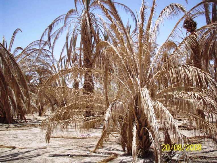
4 Consequences of over-pumping 1. GW salinization due to seawater intrusion 2. Higher pumping costs 3. Inter-generational externalities: changes in GW stock and quality

5 Oman s location Saudi Arabia UAE

6 The Batinah Coastal Plain Al Suwayq Muscat

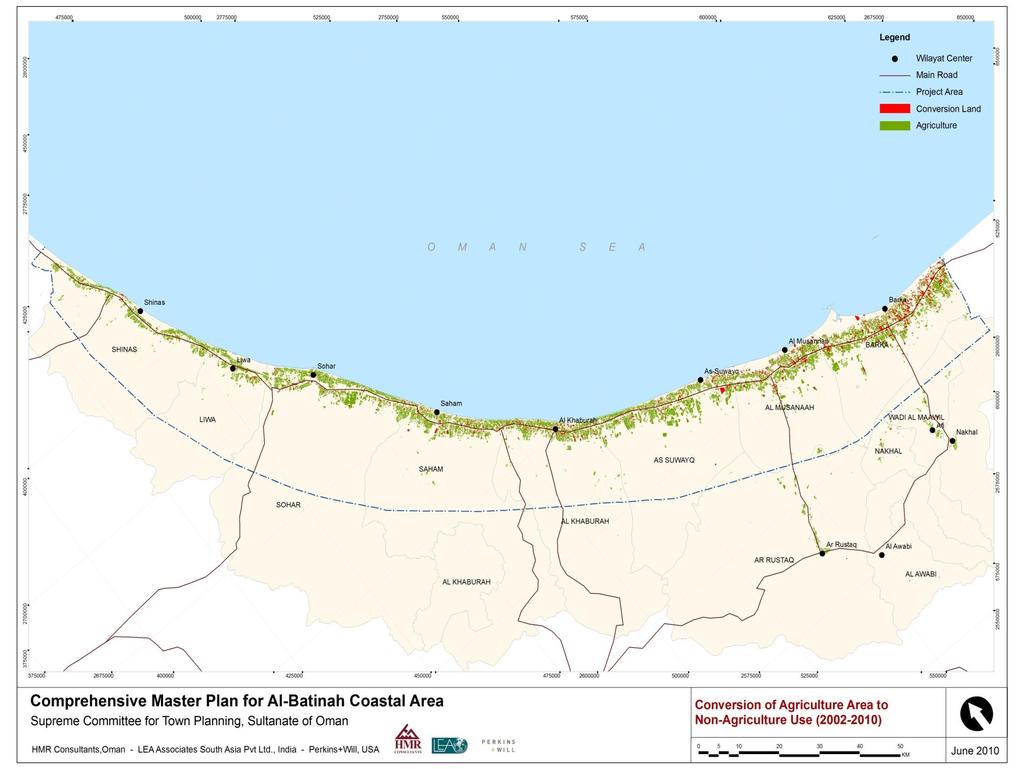
7

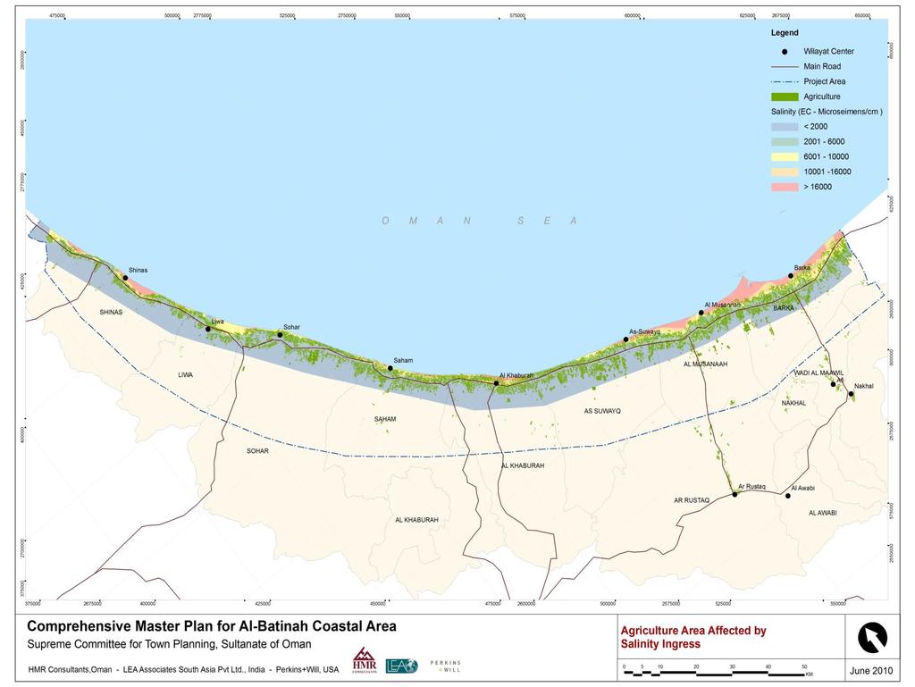
8 Observed Salinity km km km 2010 salinity observations (Al Barwani & Helmi 2006)

9 3 decades of efforts to address GW over-pumping and seawater intrusion Main measures adopted by the government since the 1990 s: a vast subsidy program of irrigation modernization a freeze on drilling new wells delimitation of several no-drill zones a crop substitution program re-use of treated wastewater and construction of recharge dams But no major success to stop the salinization of the aquifers or water level drawdown

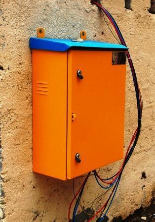
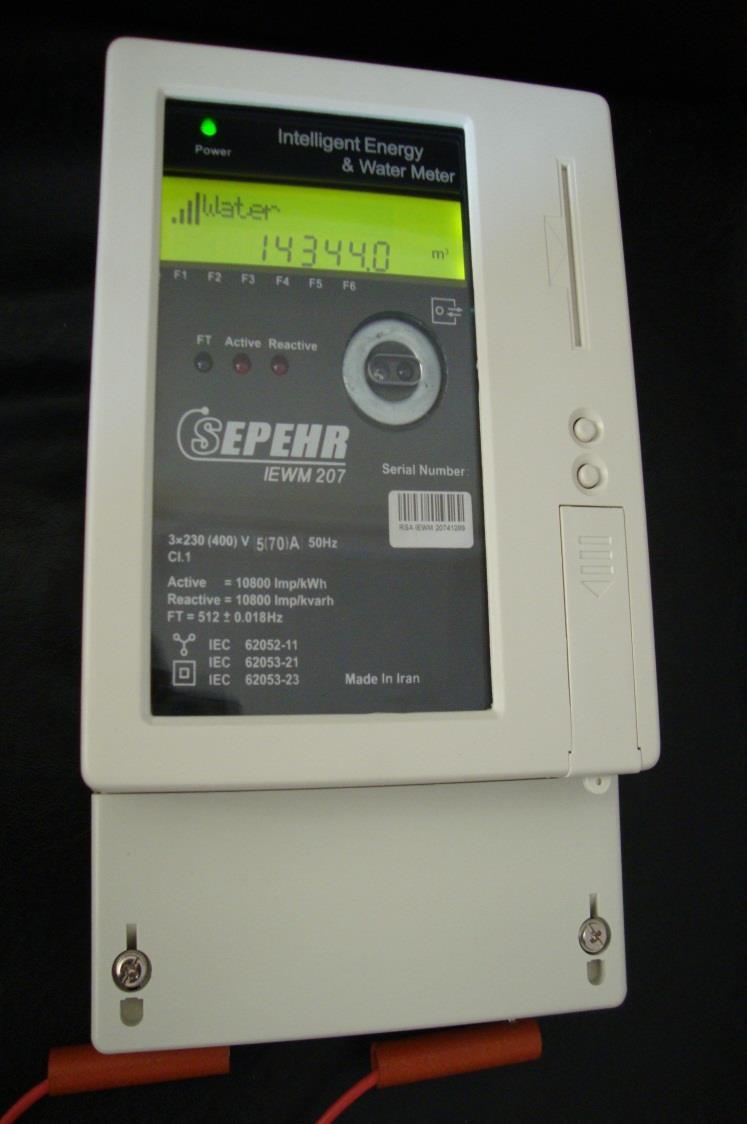
10 In 1995 a regulation laid the ground for GW quotas Early studies suggested that: cost of traditional flow metering was prohibitive and that cheating is easy majority of Omani farmers have been found to be open to quotas, provided that: groundwater remains free of charge the quota covers the crops water requirement the quota is enforced without favoritism To overcome the major practical challenges of metering, smart electricity-water meters have been equipped with modems to facilitate GW use control and monitoring without creating a financial burden for the farmers and allowing for cheating detection 40 Farms were equipped since June 2013

11

12 Wireless Smart Irrigation System Developed Designing the appropriate quotas (soil type, crops ) Subjective decisions about when and how much to irrigate causing inefficiency Keeping cropped area while reducing pumping? Date Palm Irrigation frequency Bubbler/Drip system Once a Week 6% Surface/Flood system Twice a Week 47% 17% After two days regularly 6% After one day regularly 6% Daily 35% 83% Total 100% 100

13 Role of SI water on pumping and productivity? Wireless Automated SI System developed based on a network of moisture sensors, temperature sensors and electro-valves distributed at farm level. Tested in Lab and in Univ. Farm Cost: $3,600/ha. 1/5 th of commercial cost Upgraded existing Drip/Sprinkler systems 15 Farms equipped since august farms with fert-igation system Objectives: 1. How much groundwater could be saved? 2. Labour saving 3. Productivity improvement 4. Feasibility, technical difficulties & adoption by farmers

14 Method A hydro-economic model that couples an aquifer MODFLOW- SEAWAT model and a dynamic profit maximization model using GAMS Long-term simulation-optimization Optimization model features: Profit, crops, land and salinity are considered at farm-level in the model Salinity is included in model via a Bayesian Inference Expectation Can be run for different management institutions (noncooperative, cooperative, regulatory interventions, ) Relatively low run-time and high accuracy for a large-scale model

15 Model s size and computation A matrix with 2 Million Rows by 3.5 Million Columns and 20 Million Non-zero variables that is solved within 18 Minutes by GAMS. The SEAWAT also takes 27 Minutes to simulate the model for 60 years. The model has 82 by 43 cells in 7 layers covering two main geological formations. An alluvium formation nearly 100 meter deep and the second is called upper fares with more 500 meters depth.

16 The Salinity Modeling in GAMS Optimization occurs in a separate environment from MODFLOW, the integration between MODFLOW and Optimization happens by a Surrogate Model which parameters are updated during the iterations that provide communication between Optimization and MODFLOW This Surrogate Model is basically a linear regression model of the following form: TDS y i,j = β i,j i,j y Q i,j α i,j NR

17 Some Tested Scenarios 1. Business As Usual (BAU): current pattern and allocation of cropping continues without change (simulation) 2. Central Planner Model (CPM): Long-term optimization with perfect foresight into consequences of pumping on salinity [COOPERATIVE] 3. Agent Based Model (ABM): Annual profit optimization with ex-post partial information on salinity [NON-COOPERTIVE] 4. Exogenous Regulatory Interventions are being evaluated The 3 first scenarios are analyzed under current irrigation system and fully converted irrigation system to modern

18 Profit in Mllions $ Results Profit CPM2-Profit $ ABM2-Profit $ BAU-Profit $

19 Million Cubic Meters Water Pumping CPM2-Water Use ABM2-Water Use BAU-Water Use

20 Hectares 8500 Cropped Area , , CPM2-Total Area ABM2-Total Area 5, BAU-Total Area

21 Lessons Learned Smart GW meters allowed online daily reading at a low cost: $2/month communication cost Resisted the high summer temperature 60 C. Comparison of crop water requirement and pumping Could be scaled up Low cost Smart irrigation system in place Results will require one more year How farmers will interact with the technology? Maintenance and problem solving? Water use efficiency per crop as SI allows daily measures of water use per crop How fert-igation will affect productivity? Centrally planned model 45% less GW pumping : Sustainable Renewable Flow = 170 Mm 3 800% profit: there is room to improvement Cropped area decreased from 8,100 to a cst 6,800 Ha

22 Agent Based Model Lessons Learned Profit mimics the CPM for few years then keeps decreasing over the years: Agents have only ex-post on-farm information on salinity Water use decreases compared to CPM from year 2045 after 2045, the salinity of groundwater in ABM gets so bad that the model can no longer use the water up to the CPM volume 170 Mm 3 Sustainable renewable flow is 91 Mm 3 Cropped area goes down to only 5,200 ha by 2075

23 very high salinity high salinity moderate salinity low salinity freshwater

24 Acknowledgement and Thanks Research Council of Oman & Sultan Qaboos University for the funding of this project RSA electronics for the subsidy, provision and free installation and of the 40 smart electricity meters Co-investigators and technicians team

25

26 The Salinity Model Specifications The TDS is total dissolved solids, the beta and Alfa are two unknown factors depending on location i and j and NR is yearly natural recharge The variation of TDS is modeled by the above equation which considers: Salinity variation at one point is dependent on pumping in all points (The first term) If there is no pumping then it is expected that salinity improves (the second term) In NR the Natural Recharge to our modeled region is now 59 MCM per year The parameters of this model (Alfa and Beta) are not fixed at first, they are updated and become more accurate by iterations The Updating process is done by Bayesian Inference Method

27 The Bayesian Inference (Expectation) Model The process starts with an initial value then the parameters values are updated according to MODFLOW simulation results in each iteration, Thus more info is produced about the salinity and pumping and the parameters get updated with more data leading to higher accuracey This simple Bayesian method considers the previous iteration value of the parameter and its current estimation and make and average of them as shown below: β iter+1 i,j = iter β i,j iter + β i,j iter + 1 Iter is the iteration, Beta is the parameter and the Beta-hat is the current estimation of Beta based on current simulation of MODFLOW

28 The Bayesian Inference (Expectation) Model The BIM instead of a simple regression parameter estimation is making use of the past and new data so all information is used according to Bayes assumption that future realization is relying on past observations. R 2 is used to compare the BIM-regression and MODFLOW. Due to nonlinearity in groundwater processes R 2 = 0.7 still good for predicting a nonlinear model by linear model.