Identifying Priority Subwatersheds : A Case Study. D. Saraswat, P. Tacker and N. Pai Department of Biological and Agricultural Engineering

Transcription

1 Identifying Priority Subwatersheds : A Case Study D. Saraswat, P. Tacker and N. Pai Department of Biological and Agricultural Engineering

2 L Anguille River Watershed Case study to demonstrate process to help identify priority subwatersheds L Anguille River Watershed (LRWS) has TMDL for NPSrelated impairments Utilize the current data 12-digit Hydrologic Unit Code boundaries SSURGO data for all 75 counties Land Use/Land Cover (LULC) for 2006 NHD High resolution stream layer

3 L Anguille River Watershed Scale Effect 8-digit HUC- Area 2429 km 2 10-digit HUC Area between 306 km 2 to 783 km 2 12-digit HUC Area between 47.1 km 2 to km 2

4 Why Size of Subwatershed Matters? Geomorphologic resolution of sub watersheds does not significantly affect streamflow (CN independence) 1 increases by 4% on average (subsurface flow and transmission loss as subwatershed size ) Sediment load as subwatershed size ( MUSLE- subwatershed loading- implicit delivery ratio, f(peak runoff rate (drainage area))) Sediment routing= f(channel length, channel dimensions) Mineral N and Mineral P concentrations as subwatershed size 1 (Bingner et al., 1997 and Jha et al.,2004)

5 Presentation Outline L Anguille River Watershed (LRWS) Impairment, TMDL, sources and causes Model simulate processes Data input and sources Model setup Selection of variables?(sensitivity analysis) Calibration and validation Presentation of Prioritized watersheds Input Data Limitations Riparian buffer along L Anguille River and major creeks

6 L Anguille River Watershed (LRWS) East Central Arkansas ecoregion of Mississippi Delta USGS Hydrologic Unit Code and Arkansas Department of Environmental Quality (ADEQ) Planning Segment 5B Drains 938 mi 2 (2,429 km 2 ) Encompasses portions of Craighead, Cross, Lee, Poinsett, St. Francis, and Woodruff Brushy Creek Ditch, First Creek, Second Creek, Larkin Creek and Caney Creek- largest tributaries

7 L Anguille 2006 Land Use Total Area under row crops (70%) soybean (42.3%), rice (14.9%), cotton (6.6%), corn (3.3%), wheat (3.3%), Forest (21.2%), Pasture (2.6%), Urban and transportation (4.4%), Water (1.4%) (Source: Center for Advanced Spatial Technologies (CAST), 2006)

8 Impairment, TMDL and Sources 2008 Impairment 98 miles of the L Anguille river does not support aquatic life Excess sediment causes impairment Highest sediment load seasonal Spring (February to April) and summer (July to October) TMDL to reduce sediment 40% in spring 38% in summer Source of impairment Drainage of the lowland areas - ditching and channelization Silt loads carried into the streams from row crops

9 Policy Goals Goal Effective and efficient control of NPS pollution Approach Assess using sub-watersheds Identify sub-watersheds facing greatest threats from NPS pollution Policy Objective Prioritize subwatersheds for targeted projects using CWA section 319(h) incremental funds

10 Why Models Assist Policy Makers? Models simulate characteristics and processes of a water body through mathematical equations in a way that approximates reality Physical Chemical Biological Models reflect our understanding of watershed systems Quality is understanding dependent Need to use models responsibly Acknowledge limitations of model while using its strengths to make informed policy and project decisions

11 Comparative studies* - AGNPS, AnnAGNPS, HSPF, MIKE SHE, SWAT etc. Study criteria - represent practices and support total maximum daily load (TMDL) development. SWAT strengths Greatest number of management alternatives for modeling agricultural watersheds Global user base Why use SWAT Model? * Borah and Bera (2003, 2004) and Kalin and Hantush (2003)

12 SWAT Philosophy Physically based Readily available model inputs Comprehensive- Process interactions Simulate management Continuous time, daily time step Distributed parameters

13 How Model Mimic Watersheds? SWAT calculations based on watershed mass balance Water in = Water out The SWAT model simulates hydrology as a two-component system: 1.Land phase: processes = rainfall, evaporation, transpiration, infiltration, runoff, etc 2.Routing phase: processes = water, sediment and pollution flow in river.

14 For smallest modeling scale, SWAT models Weather Hydrology Plant growth Erosion Nutrients (N, P) Pesticides Management Land Phase Modeling (Source: Neitsch et al. 2005)

15 Nitrogen Balance (Source: Neitsch et al. 2005)

16 Phosphorus Balance (Source: Neitsch et al. 2005)

17 Pesticide Fate and Transport (Source: Neitsch et al. 2005)

18 Plant Growth Variables: Leaf area, Light interception, Biomass production, Stress simulation Processes: Water balance, Nutrient cycling, Temperature responses Differentiates: Woody and non woody species (Source: Neitsch et al. 2005)

19 Routing Phase Modeling Main Channel Water Sediment Nutrients Pesticides (Source: Neitsch et al. 2005) Reservoirs Water balance Sediment Nutrients Pesticides

20 Analytic Objectives Use most current spatial data 1 and SWAT to: Calibrate and validate SWAT model for12-digit HUC Prioritize 12-digit HUC sub-watersheds 2 based on percentile ranking developed using SWAT model output sediment yield cartographic modeling Geospatial analysis 3 for potential source assessment 1 ArcSWAT version Obj in NPS Mgt. Plan , page Obj in NPS Mgt. Plan , page 11.7

21 Spatial Data Input

22 Management Data Crop rotation Timing & Frequency of tillage Planting date Timing and rate of fertilizer application Irrigation Pesticides Harvesting date Tabular Data Input

23 Tabular Input Data- Management Data from research verification reports Tillage dates and frequencies Planting/harvesting dates Irrigation dates and amount Pesticide/Fertilizer dates and amount Example of fertilizer recommendation for rice fields for each county in 2004

24 Tabular Input Data- Point Sources Facility Name HUC_12 County Nearest City Latitude Longitude _ Hunters Glen Owners Assoc. 101 Craighead Jonesboro City of Harrisburg 104 Poinsett Harrisburg Crowley's Ridge Water Assoc. 201 Poinsett Harrisburg Vannadale-Birdeye Water Assoc. 202 Cross Cherry Valley City of Cherry Valley 203 Cross Cherry Valley Cross County High School 203 Cross Cherry Valley Polyone Corp. 401 Cross Wynne Mueller Industries, Inc 401 Cross Wynne Mueller Copper Tube Products 401 Cross Wynne City of Wynne 402 Cross Wynne Andrews Trailer Park 402 Cross Wynne Forrest City School - Caldwell 409 St. Francis Forrest Entergy - Hamilton Moses Plant 502 St. Francis Palestine City of Forrest 503 St. Francis Forrest City of Palestine 504 St. Francis Palestine City of Marriana - Pond B 508 Lee Marianna Magna Lomason Inc. 508 Lee Marianna City of Marriana - Pond A 508 Lee Marianna Point Sources located in 12 subwatersheds Average daily loadings for the following obtained water, sediment, ammonia, Carbonaceous biochemical oxygen demand dissolved oxygen and phosphorus

25 Model Input Data Source Data type Scale Data Provider Description Topography 30 m USGS Digital Elevation Model Land Use/ Land Cover (LULC) 30 m Center for Advanced Spatial Technologies (CAST) Soil 1:24000 United States Department of Agriculture Natural Resources Conservation Service (USDA NRCS) Stream network 1:24000 National Hydrography Dataset USGS (NHD USGS) 2006 LULC Soil Survey Geographic (SSURGO) database High resolution stream reaches (February, 2008) Weather 4 Stations NCDC 27 years (1981 to 2007) of daily temperature and precipitation Stream flow USGS Gage stations at Colt, AR and Palestine, AR( ) Sediment and nutrients Point source pollution Crop management information USGS and ADEQ Total suspended solids and total P ( ) 18 facilities ADEQ Yearly flow, sediment and nutrients ( ) County level UACES Fertilizer and irrigation application rates and timings; tillage, planting and harvesting information

26 Model Setup Methodology Divide the SWAT model building process into modules At each step, document decisions taken and assumptions made

27 SWAT Model Setup Note: Dotted arrow indicates iteration if avg. observed and avg. simulated values are within ±15%

28 Watershed Delineation User-defined User defined method uses a polygon type GIS layer to defined subwatershed boundaries

29 Rationale for User Defined Watershed Delineation Use the 12 digit HUC boundary Enhances reproducibility of this model Results in fairly equal areas of subwatersheds

30 Soil Input SSURGO data from NRCS is at higher spatial level than STATSGO

31 Slope Input Multiple slope categories calculated from elevation layer

32 Rationale for HRU Definition No universal guidelines available. Used Gitau et al. (2007), for same watershed 5% and 10%, respectively for landuses and soil account for the most (95% and 90%) of the subwatersheds The number of HRUs are reduced by a factor of ten compared to 0% landuse and soil scenario, (982 HRUs as opposed to 9115 HRU)- increases computational efficiency

33 Hydrologic Response Unit HRU Defined A landuse/soil/slope above a user-defined threshold within a sub-watershed assigned a unique HRU Stream flow accuracy was much greater when using multiple HRUs as opposed to dominant method 1 1 Haverkamp et al. 2002

34 Weather Data Variables: Min-Max Temp(), Rainfall (mm), Solar Radiation(MJ/m 2 ), Relative Humidity (%), Wind Speed (m/s) Stations: Jonesboro, Beedeville, Marianna, and Wynne Central SWAT database updated with gage station locations Data from NCDC preprocessed into individual dbf files for each parameter and station

35 Runoff Measurement SCS-CN method is suitable when daily rainfall data is available while Green and Ampt method is for sub-daily rainfall

36 Potential Evapotranspiration (PET) Measurement Penman-Montieth is suited for those watersheds where temp, rainfall, solar radiation, wind, and RH is available.

37 Channel Routing Variable Storage Muskingum method is based on inflow and outflow of the reach

38 Management Data Input Typical crop management operations scheduled for a rice-soybean rotation practice Year Month Day Operation Crop Fertilizer applications (N and/or P) RICE Plant/begin. growing season RICE Pesticide application RICE Irrigation operation RICE Harvest and kill RICE Plant/begin. growing season SOYB Pesticide application SOYB Irrigation operation SOYB Harvest and kill SOYB

39 Model Evaluation Protocol Five components of model evaluation: Model examination, Algorithm examination, (The first two components ensure the model simulates the necessary processes and verifies that appropriate numerical techniques were used and coded correctly. ) Data evaluation: availability and quality of data for model inputs and for model evaluation. Sensitivity analysis: identify those parameters having the most influence on the model estimates. Validation: if the model adequately represents the system by comparing model predictions to independent, observed data. (Source: American Society for Testing and Materials, 1984))

40 Advantages of Standard Protocol Reduce potential modeler bias Provide a road map to follow Allow other to repeat the study Improve acceptance of model results

41 Initialize Model Run SWAT has - twenty six variables for flow components, - six for sediment, and - nine for water quality, these variables can have different values- HRU Field Experiment- cost prohibitive, physical variability, interaction and scale. Initial values determined by calibration process (Eckhardt and Arnold 2001, Rouhani et al. 2007).

42 Importance of Calibration What: The iterative process of adjusting or estimating variables using known input and output Use: A robust calibration procedure should result in realistic parameter values that provide the best agreement between simulate establishes the model s ability to represent watershed processes. d and observed values. (Source: American Society for Testing and Materials, 1984))

43 Flow Calibration

44 Sediment Calibration

45 Sensitivity Analysis for Variables Determination The relative influence of input variables on predicting total flow, sediment, and TP yield was ascertained. A total of 41 different input variables relating to flow, sediments, and TP yield were selected for the analysis. Latin Hypercube (LH, McKay et al. 1979, McKay 1988) sampling method combined with One-factor-At-a-Time (OAT, Morris 1991) The starting point for each parameter was chosen using LH sampling technique. The numbers of model executions: 420 The input parameters were ranked based on the relative magnitude of effect they had on the respective output variable.

46 Performance Acceptance Criteria The model performance for streamflow, sediment, and TP were evaluated as follows: R are considered acceptable 1 E = 1.0 indicates a perfect prediction, while negative values indicate that the predictions are less reliable than if one had used the sample mean instead. Performance Rating E PBIAS (%) Streamflow Sediment TP Very good 0.75 E 1.00 PBIAS ±10 PBIAS ±15 PBIAS ±25 Good 0.65 E 0.75 ±10 PBIAS ±15 ±15 PBIAS ±30 ±25 PBIAS ±40 Satisfactory 0.50 E 0.65 ±10 PBIAS ±25 ±30 PBIAS ±55 ±40 PBIAS ±70 Unsatisfactory E 0.50 PBIAS ±25 PBIAS ±55 PBIAS ±70 1 Santhi et al., 2001

47 Model Output Assessment Subwatershed HRU Reach SWAT output written to a database at three levels Subwatershed (sub) Reach (rch) HRU (hru) Measured data available for subbasin # 18 (USGS gage at Colt) Data from each table extracted for subbasin # 18 and compared with relevant measured data

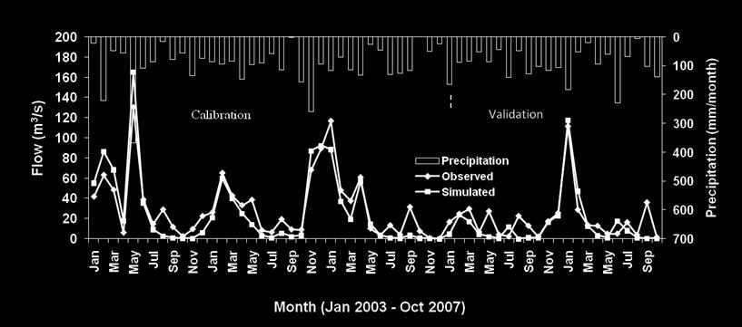
48 Streamflow Simulation

49 Sediment Loading Simulation Calibration Validation

50 Total Phosphorus Simulation Calibration Validation

51 Model Performance Assessment Results from Colt USGS Station Evaluation Criteria (measure) Total Flow Sediment Yield TP Yield Calibrated Validated Calibrated Validated Calibrated Validated R (1) 0.71 (1) E 0.67(1) 0.51 (1) -0.04(4) (1) (4) (4) PBIAS 6 (1) -8.19(1) 24.64(2) (1) 9.14 (1) -41(3) Measure: 1-Very Good, 2-Good, 3-Satisfactory, 4-Unsatisfactory, Moriasi et al. (2007)

52 Identification of Priority Watersheds- Percentile Percentile ranking was calculated based on monthly sediment and TP yield predicted by the SWAT model Importance: Calculate the relative standing of a sub watershed compared to others Decision Criteria: The sub-watersheds that produced a percentile of 80% and above were then selected and color coded to display critical watersheds For e.g., a sediment yield percentile of 80% for a particular subwatershed would imply that 80% of sub-watersheds produced sediment yields lesser than this sub-watershed

53 Percentile Ranking Calculation Steps : 1.Arrange the subwatershed number and SWAT simulated data (e.g. mean sediments) in two columns 7 2. Sort the table from low to high based on mean sediment 24% of subwatersheds have sediment loading lesser than subwatershed # 9 3.Calculate the number of data values that fall below a particular number and divide by 30 (total number of subwatersheds) For e.g. 24 = 7 / 30

54 Priority Subwatersheds- Percentile Basis Area: approx.12.% Sediment contribution: approx. 34% Area: approx. 6% TP contribution: approx. 60 %

55 Identification of Priority Watersheds- Sediment Average soil loss due to erosion from croplands in Arkansas: 7.65 t ha -1 yr -1 (3.1 t ac -1 yr -1 )(NRCS, 2003) Serial Soil erosion Soil erosion range, t ha -1 yr -1 No. class 1. Slight Moderate Critical >7.66

56 Identification of Priority Watersheds- Cartographic Causes (forest cover (FC) and drainage density (DD)) and effect (water quality parameter, sediment (SD), TP) The ranges were divided into four quartiles. Scores ranging from 1 to 4 based on the ranges of each variable. 1= lowest sediment load, high forest cover, lowest drainage density and lowest TP 4= highest sediment loads, lowest forest cover, highest drainage density and highest TP Y = SD+FC+DD+TP Score range= A score of 12 and plus critical subwatersheds

57 Comparison of Priority Watersheds Subwatershed # Frequency

58 Limitations in Precipitation and Monitoring Station Data Precipitation is regarded as highest source of uncertainty in hydrologic modeling Wind loss- 2-10%, Difference between gage-based areal mean and the true areal mean Several months of sediment and water quality data was missing USGS Colt- 13 out of 58 months (sediment) USGS Colt- 31 out of 58 months (Nutrient data) Palestine ADEQ- 5 and 6 months, respectively (sediment and nutrient data)

59 Uncertainty in LULC Data Level one categories: Water- 96.8%, Urban- 92.2% Forest- 91.9%, Barren Land- 85%, Cropland %, Pasture- 84.4%, Woody/herbaceous- 71.5% Overall average map accuracy- 86.7% (Source: Gorham and Tullis, 2007)

60 Summary & Conclusions The model was calibrated for the period Jan 2003 to Dec 2005 and validated for the period Jan 2006 to Oct Annual and monthly simulated flow, sediment, and TP were satisfactorily close to the observed values. The calibrated monthly results for sediment and TP were then used to identify critical sub watersheds. Rankings served to show those sub watersheds that had high sediment and TP losses and were most likely to suffer with water quality threats. These are the probable watersheds that require closure monitoring and follow up actions

61 Geospatial Analysis for Source Identification- Riparian Buffer D. Saraswat, D. Traywick and N. Pai Department of Biological and Agricultural Engineering Riparian buffers have been recognized as important landscape features that provide Unique habitat for many wildlife species 1 Filtering capabilities for removing nutrient pollutants from agricultural runoff and urbanized (impervious) areas before they reach waterways 2 Mapping of riparian buffer vegetation has not been systematically accomplished across many watersheds 2 1(Iverson et al., 2001) 2 (Cooper et al., 1987; Correll, 1997; Lowrance et al.,1997; Weller et al., 1998)

62 Riparian Buffer- Analytic Objective The primary goal of this study was to complete an inventory of riparian buffers along L Anguille river and it s major tributaries. The central premise of the study was that existing riparian buffer cover can play an effective role in maintenance and enhancement of water quality The extent to which buffer cover exists may dictate the needs or opportunities for future conservation efforts

63 Riparian Buffer- Input Data and Issues 2006 natural color imagery Stream layer- NHD Plus, ADEQ 2006 LULC Image ADEQ NHD Plus Edited

64 Riparian Buffer- Data Issues Approx. 360 km (225 miles) of streams data was manually created ADEQ NHD Plus Edited

65 Riparian Buffer- Analysis Criteria Land Slope, % Riparian Forest Buffer, ft Filter Strip minimum widths, ft Total combined width Cropland Pastures Forestry * * * * * Note: When the filter strip is located on a soil that falls in Hydrologic group D, an additional width of 25 % should be added to the minimum width 1 Existing riparian buffers were defined as areas of either forest or grass vegetation lying within a 45 m (147.5 ft) parallel band directly adjacent to center line of Major River and Five Creeks 1 Rich Joslin, NRCS

66 Riparian Buffer Status - LRWS Condition L'Anguille River First Creek Second Creek Brushy Creek Ditch Larkin Creek Caney Creek No. of ADEQ reaches % buffer cover % buffer cover % buffer cover % buffer cover % buffer cover Average buffer cover 82% 77.20% 80.70% 55.50% 67.50% 23.60%

67 Riparian Buffer Status - Visuals

68 Riparian Buffer Status - LRWS

69 Summary & Conclusions The existing stream layers from NHD Plus and ADEQ require editing for buffer inventory analysis On overall basis, the total length under riparian buffer cover stretching 22.5 m (approx. 74 ft) on each side from the stream center line varied from 23.6% (Caney Creek) to 82% (L Anguille River) The entire length of Caney Creek had less than 50% buffer area under riparian cover and was followed by Brushy Creek (28%), Larkin Creek (15%), First Creek (13%), Second Creek (11%) and L Anguille River (6%), respectively The knowledge derived from this inventory could be used for conservation planning or placement of future buffers

70 Acknowledgments

71 THANKS Questions?