AGRICULTURE FORESTRY AND OTHER LAND USE (AFOLU)

Transcription

1 Task Force on National Greenhouse Gas Inventories AGRICULTURE FORESTRY AND OTHER LAND USE (AFOLU) Sekai Ngarize and Baasansuren Jamsranjav IPCC TFI TSU IPCC Expert Meeting to collect EFDB and Software user s feedback March 2015 Windhoek, Namibia

2 Outline Introduction IPCC Guidelines for Agriculture and land-use AFOLU 3A. Livestock 3B. Land 3C. Aggregate sources and non-co 2 emissions on land Cross-cutting issues Exercise

3 Introduction Land use change and management have a significant influence on the greenhouse gas concentrations in the atmosphere. Processes accounting for emissions and removals in the biosphere are: photosynthesis, respiration, decomposition, nitrification/de-nitrification, enteric fermentation, and combustion that are driven by the biological activity and physical processes. AFOLU represents 20-24% of net anthropogenic emissions, equivalent to 10-12GtCO 2 eq/yr (AR5 based on the 2010 GHG inventory datasets). A significant proportion of GHG emissions/removals in the AFOLU sector come from developing countries

4 Terrestrial sources/sinks of GHGs Photosynthesis Oxidation Methanogenesis Methanogenesis Oxidation Nitrification & denitrification

5 Evolution of IPCC Guidance on agriculture and land-use 1996 IPCC GLs Agriculture and Land Use and Change and Forestry (LUCF) separate sectors Only the most important activities resulting in GHG emissions/removals Implicit assumption about estimating emissions and removals only over lands subject to human intervention Only accounted for aboveground biomass and soil C pools GPG & GPG-LULUCF Agriculture and Land Use, Land-use Change and Forestry (LULUCF) separate sectors Provides good practice and uncertainty management guidance Now includes all land use emissions/ removals split into six land-use categories from all pools Explicit Use of managed land as a proxy for anthropogenic emissions/removals 2006 IPCC Guidelines Agriculture and Land Use and Change and Forestry (LUCF) combined into a single sector Agriculture, Forestry and Other Land Use (AFOLU) Same approach as GPG-LULUCF Retained use of managed land Inclusion and consolidation of several previously optional categories Refinement of methods and improved defaults

6 Evolution of IPCC Guidance on Agriculture and LUCF/LULUCF LUCF Land Use Change and Forestry 1996 Revised IPCC Guidelines LULUCF Land Use, Land-use Change and Forestry GPG for LULUCF 2003 AFOLU Agriculture, Forestry and Other Land Use, 2006 IPCC Guidelines 5A Changes in Woody Biomass stocks 5B Forest & Grassland Conversion 5C Abandonment of Managed Lands 5D CO2 Emissions & Removals from Soils Forest Land Cropland Grassland Wetlands Settlements Other Land 3B1 Forest Land 3B2 Cropland 3B3 Grassland 3B4 Wetlands 3B5 Settlements 3B6 Other Land 3B Land 5E Other 3D1 Harvested Wood Products Harvested Wood Products Harvested Wood Products From Above Agriculture Land Use Change and Forestry 1996 Revised IPCC Guidelines 4A Enteric Fermentation 4B Manure management 4C Rice Cultivation 4D.Agricultural Soils 4E Prescribed Burning of Savannas 4F Burning of Agricultural Residues 4G Other Agriculture GPG and Uncertainty Management GPG 2000 Enteric Fermentation Manure Management Rice Cultivation Agricultural Soils Prescribed Burning of Savannas Burning of Agricultural Residues Other 3A1 Enteric Fermentation 3A2 Manure management 3C2 Liming 3C7 Rice Cultivation 3C4 Direct N2O from Managed Soils 3C5 Indirect N 2 O from Managed Soils 3C1 Emissions from Biomass Burning 3C3 Urea Application 3C6 Indirect N 2 O from Manure Management 3C8 Other 3A Livestock 3C Aggregate sources and non-co2 emissions from land

7 Agriculture Forestry and Other Land Use (AFOLU) AFOLU 3A. Livestock 3B. Land 3C. Aggregate Sources and Non- CO 2 Emissions on Land

8 3A. LIVESTOCK

9 3A. Livestock emissions 3A. Livestock 3.A.1Enteric Fermentation 3.A.2 Manure Management CH 4 N 2 O CH 4

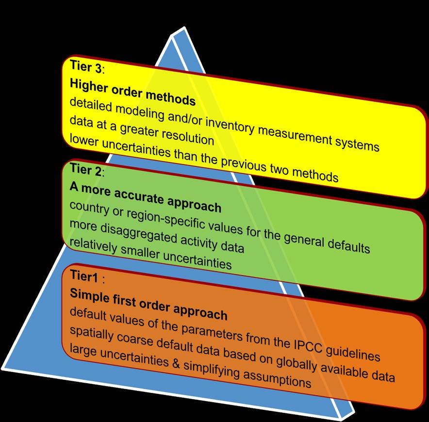
10 Three methodological Tiers

11 Livestock population and feed characterization It could be necessary to use different methodological tiers for different source categories for the same livestock types. It is a good practice to identify the appropriate method for estimating emissions for each source category, and then base the livestock information (characterisation) on the most detailed requirements identified for each livestock species. Characterization may undergo iteration based on the needs assessed during the emissions estimation process. Basic Characterization Enhanced Characterization Used for Tier 1 methods Livestock species and categories Annual population Dairy cows and milk production Used for Tier 2/3 methods Definitions for livestock subcategories Livestock population by subcategory Feed intake estimates

12 Steps to livestock characterization Identify livestock species that contribute to more than one source category Typically: cattle, buffalo, sheep, goats, swine, horses, camels, mules/asses, and poultry Review the emission estimation method (tier) for each relevant source category (EF & MM) Existing inventory or Tier 1 methods Identify the most detailed characterisation required for each livestock species Basic characterization sufficient for Tier 1 methods for both EF & MM but Enhanced characterization is required if Tier 2 is required for either of them.

13 Decision tree for livestock population characterisation

14

15 Gross energy Animal performance and diet data are used to estimate feed intake, which is the amount of Gross Energy (MJ/day) an animal needs for maintenance and for activities such as growth, lactation, and pregnancy. Total net energy requirement for animal performance and feed digestibility data are used to estimate the Gross Energy (GE). The feed intake in kg day -1 should be calculated by converting from GE in energy units to dry matter intake (DMI), by dividing GE by the energy density of the feed.

16 Feed intake estimates Tier 2 emissions estimates require feed intakes for a representative animal in each subcategory. Feed intake is typically measured in terms of gross energy (e.g., mega joules (MJ) per day) or dry matter (e.g., kilograms (kg) per day). Dry matter is the amount of feed consumed (kg) after it has been corrected for the water content in the complete diet. For all estimates of feed intake, good practice is to: Collect data to describe the animal s typical diet and performance in each subcategory; Estimate feed intake from the animal performance and diet data for each subcategory.

17 Net Energy for lactation (NEl) Net Energy for work (NEwork) Net Energy for pregnancy(nep) Net Energy for activity (NEa) Net Energy for growth (NEg) Net Energy for maintenance (NEm) Net Energy for animal performance Net energy for wool (NEwool)

18 Decision Tree for livestock categories 1. To be repeated for each livestock species and gas 2. Significant livestock species account for 25-30% or more of emissions from the source category

19 Enteric Fermentation: Tier 1 method Where: Emissions = methane emissions from Enteric Fermentation, Gg CH 4 yr -1 EF(T) = emission factor for the defined livestock population, kg CH 4 head -1 yr -1 N(T) = the number of head of livestock species / category T in the country T = species/category of livestock Where: Total CH 4 Enteric = total methane emissions from Enteric Fermentation, Gg CH 4 yr -1 Ei = is the emissions for the ith livestock categories and subcategories

20 Enteric Fermentation: Tier 2 Method Where: EF = emission factor, kg Gg CH 4 yr -1 GE = gross energy intake, MJ head -1 day -1 Ym = methane conversion factor, per cent of gross energy in feed converted to methane. The factor (MJ/kg CH 4 ) is the energy content of methane

21 Choice of emission factors Tier 1 method requires default EFs for the livestock subcategories according to the basic characterization scheme. Tier 2 methods require country-specific EFs estimated for each animal category based on the gross energy intake estimated using the detailed data on animal feed and performance and methane conversion factor for the category.

22 Choice of activity data Tier 1 method requires collection of livestock population data according to basic characterization. Tier 2 method requires animal population data according to single livestock enhanced characterisation depending upon the most disaggregated data requirements between enteric fermentation and manure management categories.

23 Enteric fermentation: Calculation steps for all Tiers Step 1: Divide the livestock population subgroups and characterize each subgroup preferably using annual averages (production cycles and seasonal influences on population numbers. Step 2: Estimate emission factors for each subgroup in kg CH 4 /animal/yr Step 3: Multiply the subgroup emission factors by the subgroup populations to estimate subgroup emission, and sum across the subgroups to estimate total emission.

24 Manure Management (CH 4 ) CH 4 is produced during the storage and treatment of manure, and from manure deposited on pasture. Most favorable conditions for CH 4 production are when large numbers of animals are managed in a confined area (e.g., dairy farms, beef feedlots, and swine and poultry farms), and where manure is disposed of in liquid-based systems. The main factors affecting CH 4 emissions are the amount of manure produced and the portion of the manure that decomposes anaerobically that are influenced by storage conditions (liquid/solid), retention times and temperature.

25 Manure Management (CH 4 ) (2) Where: CH 4Manure = CH 4 emissions from manure management, for a defined population, Gg CH 4 yr -1 EF(T) = emission factor for the defined livestock population, kg CH 4 head -1 yr -1 N(T) = the number of head of livestock species/category T in the country T = species/category of livestock

26 Choice of emission factors Tier 1 Default methane emission factors for manure management by livestock category or subcategory are used. Default emission factors represent the range in manure volatile solids content and in manure management practices used in each region. Tier 2 The Tier 2 method relies on two primary types of inputs that affect the calculation of methane emission factors from manure: manure characteristics and MMS characteristics.

27 Choice of emission factors (2) Manure characteristics includes: the amount of volatile solids (VS) produced in the manure VS can be estimated based on feed intake and digestibility, which are the variables also used to develop the Tier 2 enteric fermentation emission factors. the maximum amount of methane able to be produced from that manure (Bo) Bo varies by animal species and feed regimen and is a theoretical methane yield based on the amount of VS in the manure. Manure management system characteristics includes: the types of systems used to manage manure and a system-specific methane conversion factor (MCF) that reflects the portion of Bo that is achieved. Regional assessments of MMS are used to estimate the portion of the manure handled with each.

28 Choice of emission factors (3) Where: EF(T) = annual CH 4 emission factor for livestock category T, kg CH 4 animal -1 yr -1 VS(T) = daily volatile solid excreted for livestock category T, kg dry matter animal -1 day = basis for calculating annual VS production, days yr -1 Bo(T) = maximum methane producing capacity for manure produced by livestock category T, m 3 CH 4 kg -1 of VS excreted 0.67 = conversion factor of m 3 CH 4 to kilograms CH 4 MCF(S,k) = methane conversion factors for each manure management system S by climate region k, % MS(T,S,k) = fraction of livestock category T's manure handled using manure management system S in climate region k, dimensionless

29 Choice of emission factors (4) For Tier 2 method while some default values have been provided in the IPCC Guidelines, country-specific values of parameters Bo, VS and MCF should be used as far as possible as the default values may not encompass the potentially wide variations in these values according to national circumstances.

30 Choice of activity data Tier 1 method requires collection of livestock population data according to basic characterization. Tier 2 method requires two main types of activity data: animal population data single livestock enhanced characterisation depending upon the most disaggregated data requirements between enteric fermentation and manure management should be adopted. regional population breakdown according to for each major climatic zone along with the average annual temperature to select the EFs MMS usage data portion of manure managed in each MMS for each representative animal species from published literature, national surveys etc.

31 Manure Management (CH 4 ): calculation steps for all Tiers Step 1: Divide the livestock population subgroups and characterize each subgroup preferably using annual averages considering production cycles and seasonal influences on population numbers Step 2: Estimate emission factors for each subgroup in kg CH 4 /animal/yr Step 3: Multiply the subgroup emission factors by the subgroup populations to estimate subgroup emission, and sum across the subgroups to estimate total emission

32 Manure Management (N 2 O) Direct N 2 O emissions occur via combined nitrification and denitrification of nitrogen contained in the manure. The emission of N 2 O from manure during storage and treatment depends on the nitrogen and carbon content of manure, duration of the storage, type of treatment, acidity and moisture content. Indirect emissions result from volatile nitrogen losses that occur primarily in the forms of ammonia and NOx. The fraction of excreted organic nitrogen that is mineralized to ammonia nitrogen during manure collection and storage depends primarily on time, and to a lesser degree temperature.

33 Direct N 2 O from Manure Management Direct N 2 O emissions from manure management is given by Where: N 2 O D(mm ) = Direct N 2 O emissions from Manure Management in the country, kg N 2 O yr -1 N (T) = number of animals/category T in the country N ex(t) = annual average N excretion/head of species/category T, kg N animal -1 yr -1 MS (T,S) = fraction of total annual N excretion for each livestock species/category T handled in MMS, S in the country, dimensionless EF 3(S) = EF for direct N 2 O emissions from MMS, S in the country, kg N 2 O-N/kg N in MMS, S S = manure management system T = species/category of livestock 44/28 = conversion of (N 2 O-N)(mm) emissions to N 2 O(mm) emissions

34 Choice of emission factors Tier 1 Annual nitrogen excretion for each livestock category defined by the livestock population characterisation. Country-specific values or from other countries with livestock with similar characteristics IPCC defaults of N excretion rates (2006 IPCC Guidelines) could be used with typical animal mass (TAM) values Default emission factors from the IPCC Guidelines

35 Choice of emission factors (2) Tier 2 Annual nitrogen excretion for each livestock category defined by the livestock population characterisation based on total annual N intake and total annual N retention data of animals. Country-specific emission factors that that reflect the actual duration of storage and type of treatment of animal manure in each system

36 Choice of activity data Tier 1 Animal population data according to basic characterization. Default or country specific manure management system usage data Tier 2 Animal population data according to single enhanced characterization. Country-specific manure management system usage data from national statistics or independent survey

37 Step 5: For each manure management system type S, multiply its (EF 3(S) ) by the total amount of nitrogen managed (from all livestock species/categories) in that system, to estimate N 2 O emissions from that MMS. Then sum over all MMS. Calculation steps for all Tiers Step 1: Divide the livestock population subgroups and characterize each subgroup preferably using annual averages considering production cycles and seasonal influences on population numbers. Step 2: Use default values or develop the annual average nitrogen excretion rate per head (Nex(T)) for each defined livestock species/category T. Step 3: Use default values or determine the fraction of total annual nitrogen excretion for each livestock species/category T that is managed in each manure management system S (MS (T,S) ). Step 4: Use default values or develop N 2 O emission factors for each manure management system S (EF 3(S) ).

38 Uncertainty assessment There are large uncertainties associated with the default emission factors ( 50% to +100%). The uncertainty of Tier 2 EFs method will depend on the accuracy of the livestock characterisation (e.g., homogeneity of livestock categories), and their correspondence with national circumstances Accurate and well-designed emission measurements from well characterised types of manure and manure management systems can help reduce these uncertainties further. Activity data uncertainty is associated with the livestock population, manure management system usage data.

39 Completeness Livestock emission estimates should cover all the major animal categories managed in the country. For animals occurring in the country for which default data are not available and for which no guidelines are provided, the emissions estimate should be developed using the same general principles. A complete inventory should include all systems of manure management for all livestock species/categories; at a minimum Tier 1 estimates should be provided for all major livestock categories.

40 Time-series consistency Developing a consistent time series requires collection of an internally consistent time series of livestock population statistics using techniques to ensure it. To ensure time-series consistency, EFs and parameters (e.g., methane conversion factors) used to estimate emissions must reflect the change in management practices and/or the implementation of GHG mitigation measures.

41 QA/QC It is good practice to implement general quality control checks, and expert review of the emission estimates. Additional quality control checks and quality assurance procedures may also be applicable, particularly for higher tier methods e.g., Checking population data between national and international datasets (such as FAO and national agricultural statistics databases); Reviewing livestock data collection methods, in particular checking that livestock subspecies data were collected and aggregated correctly with consideration for the duration of production cycles; Reviewing EFs, parameters and activity data (e.g., MCF, MMS usage data etc.) to ensure they reflect changes in management practices and mitigation measures; Comparison of CS factors with IPCC defaults and other countries data

42 3B. LAND

43 Outline - FOLU IPCC Guidelines and use of managed land as a proxy Land use and management categories Carbon pools definitions Key IPCC principles for estimating emissions/removals Tier definitions and emission factors (EF) Decision trees Approaches to land representation and activity data (AD) Data requirements for FOLU Methodological approaches used in the estimation of emissions/removals in FOLU sector Steps in preparing inventory estimates Cross-cutting issues Exercise

44 The use of managed land as a proxy in estimating land-based emissions and removals (E/R) Factors governing E/R can be both natural and anthropogenic and can be difficult to distinguish between causal factors Inventory methods have to be operational, practical and globally applicable while being scientifically sound IPCC Guidelines have taken the approach of defining anthropogenic greenhouse gas emissions by sources and removals by sinks as all those occurring on managed land Managed land is land where human interventions and practices have been applied to perform production, ecological or social functions Managed land has to be nationally defined and classified transparently and consistently over time GHG emissions/removals need not be reported for unmanaged land

45 Six land-use categories Stock changes of C pools are estimated and reported for the six top-level land-use categories Forest Land Cropland Other land Grassland Settlements Wetland Subdivide according to national circumstances

46 IPCC Guidance on DOM and Soil C Carbon Pools Living biomass Dead Organic Matter Soil C Above ground biomass - All living biomass above the soil incl. stem, stump, branches, bark, seeds & foliage Below ground biomass -All living biomass of live roots, often excl. fine roots of less than (suggested) 2 mm dia. Dead wood -All non-living woody biomass not litter either standing, lying on the ground, or in the soil; -Incl. surface wood, dead roots, stumps larger than dia. used by country to distinguish from litter (e.g., 10 cm). Litter -All non living biomass of dia. < chosen by the country (e.g., 10 cm) lying dead above soil; - Incl. litter, fumic and humic layers & live fine roots > dia. used to distinguish below ground biomass (e.g., 2 mm). organic C in mineral and organic soils (including peat) to a specified depth chosen by country (default depth 30 cm for Tier 1 & 2 methods) incl. live fine roots if cannot be distinguished empirically

47 Land-use subcategories and carbon pools Each land-use category is further subdivided into land remaining in that category (e.g., FL-FL) and land converted from one category to another (e.g., FL-CL) for estimation of C stock changes. The total CO2 emissions/removals from C stock changes for each LU category is the sum of those from these two subcategories. 3B. Land FL CL GL WL SL OL FL-FL L-FL Biomass DOM Soils

48 Total estimates for GHG are made up of subdivisions of land use categories Land remaining in the same land use category Land converted from one category to another Total emissions from land use category

49 Key IPCC principles for estimating E/R The simplest methodological approach consists of combining information on the extent of human activity ( called activity data - AD) with coefficients that quantify emissions/removals per unit activity (AF)

50 Three methodological Tiers

51 Methodological choice- use of decision trees 1.To be repeated for each subcategory, pool and gas 2. Significant pools account for 25-30% or more of emissions/removals from the source category

52 Three approaches for Land Representation

53 Approach 1 53

54 Approach 2 54

55 Approach 3: Spatially Explicit 55

56 Ex. # 1: LU matrix: Can you fill in the missing values? Initial Final FL CL GL WL SE OL Final Area FL ?? CL GL 3 7?? WL SE OL Initial 66 44?? 20?? 5 215

57 And the answer is Initial Final FL CL GL WL SE OL Final Area FL CL GL WL SE OL Initial

58 Two basic inputs in calculating GHG inventories Activities Approaches for estimating change in area of land categories Emission Factors Tier 1: IPCC default factors Total area per category Net Changes only (Approach 1) Total area per category Estimate land conversions rates (Approach 2) Spatially explicit tracking of land conversions over time (Approach 3) GHG inventory estimates for each land category Tier 2: Country Specific data for key factors Tier 3: Modelling plus repeated measurements of key stocks through time

59 FOLU Data requirements: Activity Data, e.g., Forest land Chap 4, 2006 GL, Vol 4 i) Area of forest land remaining forest land Disaggregation according to climatic region, vegetation type, species, management, age e.t.c., ii) Area of other land category converted to forest land Disaggregation as above iii) Forest areas affected by disturbances iv) Forest area undergoing transition from one state to another v) Area of forest burnt vii) Total afforested land derived from cropland/grassland vii) Area of land converted to forest land through Natural regeneration Establishment of plantations

60 FOLU Data requirements: Activity data: Forest Land 2006 GL, Vol 4. Activity data Tier 1 Tier 2 Tier 3 - Data from national sources such - Data largely from as the Ministry of national sources such as Environment/Forests/Natural the Ministry of Resources Environment etc. - If national source unavailable, - The data on area should use international data sources such be disaggregated as FAO and TBFRA according to different - Data is normally at national plantation/forest types at aggregated level for major an appropriate scale plantation/forest categories - Verify, validate and update national and international data sources Area of forest/ plantations Harvest categories or types of wood (e.g., saw logs & veneer logs, pulpwood, & other industrial roundwood) - Data not likely to be available - Data not likely to be available - If available, national aggregate biomass harvest data to be used - Data from national remote sensing or satellite assessment sources - Data available at fine grid scales for different plantation/forest types - Geo-referenced forest area data to be used - Quantities of biomass harvested from different plantation / forest categories to be obtained and used

61 FOLU Data requirements: Activity Data: Forest Land contd. Activity data Tier 1 Tier 2 Tier 3 Commercial harvest (quantity of different harvest categories mentioned above) - National level aggregate commercial harvest statistics to be used Traditional fuelwood use Other wood use - FAO provides data in the form of roundwood - The roundwood data to be converted to aboveground (whole tree) biomass using biomass expansion ratio - Verify, validate and update the data source - FAO provides data on fuelwood and charcoal use - Verify, validate and update the data source - National level fuelwood consumption data from national sources, at aggregate level to be used - Country-specific commercial harvest data from different forest categories at resolution corresponding to Tier 3 forest/plantation categories to be used - Country-specific fuelwood extraction data for Tier 3 forest / plantation categories to be used Same approach as adopted for commercial harvest or traditional fuelwood use

62 FOLU Data requirements: Emission/Removal Factors - Forest land The key emission/removal factors include: annual biomass growth rate, carbon fraction of dry matter, biomass expansion ratio Biomass Expansion Ratios (BERs) as given in IPCC 2006 GL are required to convert commercial roundwood harvested biomass (in m 3 ) to total above-ground biomass (in tonnes) AGB:BGB ratio is required to estimate BGB using data on AGB - the conversion ratio (R), according to 2006 GL. Combining tiers Inventory experts could adopt different tiers for different emission factors AGB- Above Ground Biomass BGB- Below Ground Biomass

63 FOLU Data requirements: Emission/Removal Factors - Forest Land Emission/removal factor Annual biomass growth rate Carbon fraction of dry matter Biomass expansion ratio (BER) Tier 1 Tier 2 Tier 3 - Default values of average annual biomass growth rate to be used for each forest / plantation category from global databases - Verify, validate and update international data sources - Use country-specific data available for as many forest/plantation categories - Use default data if country-specific data is not available for a given forest/plantation category - Use default data - Use default data, if forest species-specific data are not available - Use default BER to convert commercial harvest data to total aboveground biomass removed in commercial harvest - BER requires conversion from m 3 to tons and expansion ratio to convert commercial harvest data to total biomass removed - Inventory experts encouraged to develop country-specific BERs for different plantation / forest categories - Default values to be used in the absence of national data - Use annual increment data from detailed periodic forest inventory/monitoring system - Species-specific allometric biomass functions could also be used - Use forest speciesspecific carbon fraction data obtained from laboratory estimations - Estimate BER values at species level - BERs for biomass increment, growing stock and harvest differ for a given species or a stand, requiring separate estimation

64 FOLU Data requirements: Activity Data- Cropland Activity data Area converted annually Average area converted (10-year average) Tier 1 Tier 2 Tier 3 - Gross area converted at the national level can be obtained from national sources such as the Ministry of Environment / Forests/Natural Resources - If national source unavailable, international data sources on deforestation such as the FAO and TBFRA - Normally, average annual rates of conversion are extrapolated to the inventory year - Forest/grassland area converted according to different types, available at the national level from government /ministry sources to be used - The data on area should be disaggregated according to different forest / grassland types at an appropriate scale - If direct annual estimates not available, use average annual rates of conversion - Disaggregated according to forest/grassland types and geo-referenced data from periodic satellite/remote sensing assessments could be used - Countries can use direct estimates of spatially disaggregated areas converted annually

65 FOLU Data requirements: Emission Factors- Cropland Emission factor Tier 1 Tier 2 Tier 3 Aboveground biomass before and after conversion - Use default coefficients to estimate carbon stock change in biomass, resulting from land use conversions - Default assumption is that all biomass is cleared during conversion, leading to zero biomass after conversion - Country-specific estimates of biomass stocks before and after conversion could be generated nationally - Biomass data from national forest inventory studies in different forest/grassland categories subjected to conversion - Biomass could be estimated using species-specific allometric equations - Geo-referenced biomass change data at finer spatial scales

66 FOLU Data requirements: Emission Factors - Cropland Fraction of biomass burnt on-site and off-site Fraction of biomass oxidised Carbon fraction of biomass Fraction of biomass left to decay - Use default values - Country-specific fraction of biomass burnt on-site and off-site to be generated nationally - Apportion fraction of biomass carbon loss due to on-site and off-site burning from field measurements - Use default data - Field measurements of biomass fraction burnt on-site and offsite in different forest/grassland categories subjected to conversion - Use default data, if no measurements are available - Laboratory estimation of carbon fraction for different species - Field measurements of biomass left to decay in different forest/grassland categories subjected to conversion

67 Methodological approaches used in estimation of E/R in FOLU sector- C cycle of FOLU showing flows into and out of carbon pools Living Biomass Above- Ground Biomass Harvested Wood Products Dead Wood Countries can choose to account for HWP pool Dead Organic Matter Below- Ground Biomass Litter Increase - Growth Transfers between Pools Discrete Events Fires etc Continuous Processes e.g. decay Soil Organic Matter

68 A simple first order approach in the IPCC Guidelines The IPCC Guidelines make two assumptions: A) C flux = C stocks B) Change in carbon stocks can be estimated from land use/change and management at various points in time, their impacts on carbon stocks and the biological response to them. (IPCC 2006 GL page1.6, section 1.2.1, para 3)

69 CO 2 Emissions from C stock changes on land Annual carbon stock changes as sum for all land use categories : Equation 2.1 (2006 GL, pg 2.6) ΔC LAND = ΔC FL + ΔC CL + ΔC GL + ΔC WL + ΔC SL + ΔC OL Annual C stock changes for a land-use category- sum of each stratum within category: Equation 2.2 (2006 GL, pg 2.7) ΔC LU = Σ ΔC LU i Annual carbon stock changes for a stratum of a land-use category- sum of all carbon pools: Equation 2.3 (2006 GL, pg 2.7) ΔC LUi = ΔC AB + ΔC BB + ΔC DW + ΔC LI + ΔC SO

70 Estimating C stock changes 1 2 C uptake through Growth Carbon Stock in year 1 Carbon Stock in Year 2 Disturbances Land Use type Harvest Difference between carbon stocks (Stock- Difference Method) Sum of gains and losses (Gain-Loss Method)

71 Stock-Difference Method Stock-Difference Method can be used where carbon stocks in relevant pools are measured at two points in time to assess carbon stock changes C = (C 2 C 1 )/(t 2 -t 1 ) Where: ΔC = annual carbon stock change in the pool, tonnes C yr -1 C 1 = carbon stock in the pool at time t 1, tonnes C C 2 = carbon stock in the pool at time t 2, tonnes C Equation 2.5 page 2.10, Vol 4, 2006GL

72 Gain-Loss Method Gains-Loss Method involves tracking inputs and outputs from a C pools: e.g., gains from growth (increase of biomass) and transfer of carbon from another pool (e.g., transfer of carbon from the live biomass carbon pool to the dead organic matter pool due to harvest or natural disturbances) and loss due to harvest and mortality. C = C G - C L ΔC = annual carbon stock change in the pool, tonnes C yr -1 ΔC G = annual gain of carbon, tonnes C yr -1 ΔC L = annual loss of carbon, tonnes C yr -1 Equation 2.4, page 2.9, Vol 4, 2006 GL

73 Biomass: Land Remaining in a Land-use Category Carbon stock change in biomass on Forest Land is likely to be an important sub-category due to substantial fluxes arising from management and harvest, natural disturbances, natural mortality and forest regrowth. Changes in C stocks in biomass pool can be estimated using either Stock-Change or Gain-Loss method. The Gain-Loss Method requires the biomass carbon loss to be subtracted from the biomass carbon gain. Gain-Loss Method is the basis of Tier 1 method, for which default values for calculation of increment and losses are provided in the IPCC Guidelines.

74 Annual increase in biomass carbon stocks (Gain- Loss Method), ΔC G (Land remaining in same land use category) ΔC G = Σ i, j (A i,j G TOTALi,j CF i,j ) Where: ΔC G = annual increase in biomass carbon stocks due to biomass growth in land remaining in the same land-use category by vegetation type and climatic zone, tonnes C yr -1 A = area of land remaining in the same land-use category, ha G TOTAL = mean annual biomass growth, tonnes d. m. ha -1 yr -1 i = ecological zone (i = 1 to n) j = climate domain (j = 1 to m) CF = carbon fraction of dry matter, tonne C (tonne d.m.) -1 Equation 2.9 page, 2.15, Vol 4, 2006GL

75 Average annual increment in biomass (G TOTAL ): Tier 1 G TOTAL = Σ{G W (1+ R)} Where: G TOTAL = average annual biomass growth above and belowground, tonnes d. m. ha -1 yr -1 G W = average annual above-ground biomass growth for a specific woody vegetation type, tonnes d. m. ha -1 yr -1 R = ratio of below-ground biomass to above-ground biomass for a specific vegetation type, in tonne d.m. below-ground biomass (tonne d.m. above-ground biomass) -1 ( Equation page, 2.15, Vol 4, 2006GL).

76 Average annual increment in biomass (G TOTAL ): Tier 2 &3 G TOTAL = Σ{I V BCEF I (1+ R)} I V = average net annual increment for specific vegetation type, m 3 ha -1 yr -1 BCEF I = biomass conversion and expansion factor for conversion of net annual increment in volume (including bark) to above-ground biomass growth for specific vegetation type, tonnes above-ground biomass growth (m 3 net annual increment) -1 ( Equation page 2.15, Vol 4, 2006GL).

77 Biomass carbon stocks losses (Gain-Loss Method), ΔC L ΔC L = L wood removals + L fuelwood + L disturbance Where: ΔC L = annual decrease in carbon stocks due to biomass loss in land remaining in the same land-use category, tonnes C yr -1 L wood-removals = annual carbon loss due to wood removals, tonnes C yr -1 L fuelwood = annual biomass carbon loss due to fuelwood removals, tonnes C yr -1 L disturbance = annual biomass carbon losses due to disturbances, tonnes C yr -1 (Equation 2.11, Vol 4, Page 2.16, 2006 GL)

78 Ex. # 2: Can you find the biomass C pool loss/gain? Growth = 200,000 tonnes C yr-1 Loss due to Harvest = 500 tonnes C yr-1 Natural disturbance losses= 2000 tonnes C yr-1 Fuelwood removals = 300 tonnes C yr-1

79 And the answer is ΔC G = 200,000 tonnes C yr-1 ΔC L = L wood removals + L fuelwood + L disturbance = = 2800 tonnes C yr-1 ΔC biomass = ΔC G ΔC L = 200, = tonnes C yr-1

80 Stock Change Method C = (C 2 C 1 )/(t 2 -t 1 ) C= Σ i j C A i j V i j BCEF S R i j CF i j ) C = total carbon in biomass for time t 1 to t 2 [i = ecological zone i (i = 1 to n) j = climate domain j (j = 1 to m)] A = area of land remaining in the same land-use category, ha (see note below) V = merchantable growing stock volume, m 3 ha -1 R = ratio of below-ground biomass to above-ground biomass, tonne d.m. below-ground biomass (tonne d.m. above-ground biomass) -1 CF = carbon fraction of dry matter, tonne C (tonne d.m.) -1 BCEF S = biomass conversion and expansion factor Equation 2.8 a and b, page 2.12, Vol 4, 2006GL - ( land remaining in same land use category)

81 Biomass: Land Converted to Other Land-Use Category ( tier 2 and 3) ΔC B = ΔC G + ΔC CONVERSION ΔC L Where: ΔC B = annual change in carbon stocks in biomass on land converted to other land-use category, in tonnes C yr -1 ΔC G = annual increase in carbon stocks in biomass due to growth on land converted to another land-use category, in tonnes C yr -1 ΔC CONVERSION = initial change in carbon stocks in biomass on land converted to other land-use category, in tonnes C yr -1 ΔC L = annual decrease in biomass carbon stocks due to losses from harvesting, fuel wood gathering and disturbances on land converted to other land-use category, in tonnes C yr -1 (Equation.2.15, page 2.20, Vol 4, 2006GL)

82 Initial change in biomass carbon stocks in Land Converted to Other Land-Use Category * ΔC CONVERSION = Σ i (B AFTER B BEFORE ) ΔA TO OTHERS i CF Where: ΔC CONVERSION = initial change in biomass carbon stocks on land converted to another land category, tonnes C yr -1 B AFTERi = biomass stocks on land type i immediately after conversion, t d.m.ha -1 B BEFOREi = biomass stocks on land type i before conversion, t d.m. ha -1 ΔA TO_OTHERSi = area of land use i converted to another land-use category in a certain year, ha yr-1 CF = carbon fraction of dry matter, tonne C (t d.m.) -1 i = type of land use converted to another land-use category (Equation 2.16, Page 2.20, Vol 4, 2006 GL)

83 Change in C stocks in DOM: Land Remaining in the Same Land Use The Tier 1 assumption for both dead wood and litter pools for all land-use categories is that their stocks are not changing over time if the land remains within the same land-use category. Tier 2 methods for estimation of carbon stock changes in DOM pools calculate the changes in dead wood and litter carbon pools by either Gain-Loss Method or Stock-Difference Method (GPG LULUCF provides guidance on DOM only for FL) These estimates require either detailed inventories that include repeated measurements of dead wood and litter pools, or models that simulate dead wood and litter dynamics.

84 Gain-Loss Method C DOM = [A (DOM in DOM out )] CF A = area of managed land,ha DOM in = average annual transfer into DW/litter pool (due to mortality, slash due to harvest and natural disturbance),t d.m./ha/yr DOM out = average annual transfer out of DW/litter pool, t d.m./ha/yr CF = carbon fraction of dry matter, tc/(t d.m.) (Equation 2.18, page 2.23, Vol 4, 2006 GL)

85 Stock-Difference Method C DOM = [A (DOM t2 DOM t1 )/T] CF A = area of managed land, ha DOM t1 = DW/litter stocks at time t 1 for managed land, t d.m/ha DOM t2 = DW/litter stocks at time t 2 for managed land, t d.m/ha T= (t 2 -t 1 ) = time period between the two estimates of DOM, yrs. CF = carbon fraction of dry matter, t C/(t d.m.) (Equation 2.19, Page 2.23 Vol 4, 2006 GL)

86 Change in C stocks in DOM: Land Converted to Other Land-use The Tier 1 assumption is that DOM pools in non-forest land categories after the conversion are zero, i.e., they contain no carbon. The Tier 1 assumption for land converted from forest to another land-use category is that all DOM carbon losses occur in the year of land-use conversion. For land converted to Forest Land litter and dead wood carbon pools starting from zero carbon in those pools. DOM carbon gains on land converted to forest occur linearly, starting from zero, over a transition period (default assumption is 20 years)

87 Changes in soil C stocks C ΔCSoils soils = ΔC = ΔCMineral Mineral L LOrganic Organic + ΔC + ΔCInorganic Inorganic Where: ΔC Soils = annual change in carbon stocks in soils, t C yr -1 ΔC Mineral = annual change in organic carbon stocks in mineral soils, t C yr -1 L Organic = annual loss of carbon from drained organic soils, t C yr -1 ΔC Inorganic = annual change in inorganic carbon stocks from soils, t C yr -1 (assumed to be 0 unless using a Tier 3 approach) Equation 2.24, page 2.29, Vol 4, 2006GL

88 Mineral soils Soil organic matter in soils is in a state of dynamic balance between inputs (litterfall and its decay/incorporation into the soil) and outputs (organic matter decay through respiration) of organic C. Human actions and other disturbances alter the carbon dynamics. IPCC default method assumes: Over time, soil organic C reaches a spatially-averaged, stable value specific to the soil, climate, land-use and management practices Soil organic C stock changes during the transition to a new equilibrium SOC occurs in a linear fashion The change is computed based on C stock after the management change relative to the carbon stock in a reference condition (i.e., native vegetation that is not degraded or improved)

89 Mineral soils (2) ΔC Mineral = (SOC 0 SOC (0-T) )/D (or T) SOC = (SOC REF F ND/LU F MG F I A) T = Number of years between inventories (inventory time period), years (to be substituted for D if T > D; not done in GPG-LULUCF) D= Time dependence of stock change factors (default = 20), years SOC REF = Reference C stock for a climate-soil combination, tc/ha F ND/LU, F MG, F I = Stock change factors for natural disturbance (or land use if it is not forest), management and organic matter input (GPG-LULUCF had an adjustment factor for the forest type and none for the input regime), dimensionless A = Area of the stratum of forest/land use (with a common climate and soil type), ha. Equation 2.25, Page 2.30, Vol 4, 2006GL

90 Organic Soils Organic soils have organic matter accumulated over time under anaerobic conditions. C dynamics of organic soils are closely linked to hydrologic conditions and C stored in organic soils readily decomposes in aerobic conditions following soil drainage. Loss rates of organic C vary according to climate type, drainage depth, type of organic substrate and temperature.

91 Organic Soils (2) ΔC FFOrganic = A Drained EF Drainage Where: ΔC FFOrganic = CO 2 emissions from drained organic soils, t C/yr A drained = Area of drained organic soils, ha EF Drainage =EF for CO 2 from drained organic soils, t C/ha/yr Equation 2.26, page 2.35, Vol 4, 2006GL

92 Cross Cutting issues- Uncertainty Assessment Broad sources of uncertainty are: Uncertainty in land-use and management activity and environmental data (land area estimates, fraction of land area burnt etc.) Uncertainty in the stock change/emission factors for Tier 1 or 2 approaches (carbon increase and loss, carbon stocks, and expansion factor terms) Uncertainty in model structure/parameter error for Tier 3 modelbased approaches, or measurement error/sampling variability associated with a measurement-based inventories Uncertainty can be reduced by: using higher tier methods; more representative parameter values; and AD at higher resolution.

93 Cross Cutting issues- Completeness To ensure completeness it is good practice to include all land categories, C pools and non-co 2 emissions occurring in a country. If there are omissions, it is a good practice to collect additional activity data and related emission factors and other parameters for the next inventory particularly if the category/pool is a key category. It is a good practice to document and explain reasons for all omissions.

94 Cross Cutting issues- Time-series Consistency It is good practice to ensure time-series consistency by using the same sources of data and methods across the time series. It is a good practice to recalculate emissions/removals in case there are changes in the sources of data (e.g., improved data from national forest inventories) and methods using time-series consistent methods. Some ways of ensuring time series consistency in LULUCF are: keeping track of the land transitions through a Land Use Change Matrix; Keeping track of C stocks in land-use categories before and after transitions; and Using a common definition of climate and soil types for all land-use categories.

95 Cross Cutting issues- QA/QC It is good practice to perform quality control checks through Quality Assurance (QA) and Quality Control (QC) procedures, and expert review of the emission estimation procedures. QA/QC procedures should be clearly documented for each land-use subcategory (e.g., FL-FL and L-FL etc.).

96 Set priorities for future inventories and revise KCA for future Divide all land into managed and unmanaged lands Develop a national land classification system for six LU classes Document and archive all information Report emissions/ removals in reporting tables Steps in a LULUCF Inventory Preparation Compile data on LU/LUC for each land category Estimate CO2 emissions/remov als and non- CO2 emissions at apt. Tier (KCA) S Sum CO2 emissions and removals and non- CO2 emissions for each land use and stratum Estimate uncertainties Re-estimate if higher tier recommended by KCA

97 Summary- Key messages Land use and management have significant impact on GHG E/R AFOLU E/R significant in most developing countries 2006 IPCC Guidelines refer to sources and sinks associated with GHG emissions/removals from human activities on managed land The flux of CO2 to/from atmosphere is assumed to be equal to changes in carbon stocks in existing biomass and soils Changes in carbon stocks can be estimated by establishing rates of change in land use and practices that bring about change in land use Estimating carbon stocks in land-use categories: That remain in same land use category That have been converted to another category

98 Summary - Key messages The IPCC identifies 5 carbon pools for each land use category, carbon stock changes and E/R are estimated for each of the carbon pools Use of Tier structure and land representation Choice of methods for estimation of GHG for FOLU sector Select method of estimation (equations), based on tier level selected, quantify emissions/removals for each land-use category, carbon pool The total CO2 emissions/removals from C stock changes for each LU category is the sum of those from the two subcategories Cross-cutting issues

99 Back- up slides

100 C Pools: some general observations Land remaining Land categories Tier 1 method FL- all C pools except biomass and (drained organic) soils assumed constant CL- Only DOM assumed constant (only perennial biomass considered) GL/WL/SE all pools except (drained organic ) soils assumed constant OL All C pools assumed constant. Default parameters for other C pools Gain-Loss method for all C pools except mineral soils.

101 C Pools: some general observations (2) Land remaining Land categories: Tier 2 method: No C pool is assumed constant (except for OL) Country-specific parameters with more disaggregated AD Stock-Difference method Land converted categories: Tier 1 method: No C pools is assumed constant. L-FL: DOM C stocks before conversion assumed zero L-CL/GL/SE: Biomass and DOM C stocks following conversion assumed zero; mineral soil C moves to a new equilibrium in 20 years. L-WL: Biomass C stocks following conversion assumed zero for L- Flooded Land Default parameters with AD at coarser resolution

102 C Pools: some general observations (3) Land converted categories: Tier 2 method: No C pools is assumed constant. C stocks before and following conversion can be non-zero. Country-specific parameters and more disaggregated AD. Tier 3 method: nationally specific complex methods involving modeling and/or measurements

103 Time to equilibrium in carbon pools For lands that enter the land converted category, lands stay in that category for 20 years After 20 years, land in the land converted category is removed from the land converted category and added to the Land remaining category 20 years the IPCC default for the time it takes carbon pools to reach equilibrium after land-use conversion

104 Example FL-FL CL-CL No conversion CL-FL A B A B GL-GL S-S FL-FL C D E 2000 No conversion C D E 2025 No conversion No conversion FL-CL CL-CL???? A B A B GL-CL S-S FL-FL?????? C D E C D E

105 Example FL-FL CL-CL No conversion CL-FL A B A B GL-CL S-S FL-FL C D E 2000 FL-CL CL-CL A B GL-CL S-S FL-FL C D E No conversion CL-CL C D E 2025 A No conversion CL-FL No conversion CL-CL S-S FL-FL B C D E

106 Example stratification with supporting data for Tier 1 emissions estimation methods Factor Climate (see Annex 3A.5) Soil (see Annex 3A.5) Biomass (Ecological Zone) (see Figure 4.1, in Chapter 4) Strata (examples) Boreal Cold temperate dry Warm temperate Tropical wet High activity clay Sandy Organic Tropical rainforest Tropical dry forest Management Practices (more than 1 may be applied to any land area) Subtropical humid forest Subtropical desert Temperate steppe Intensive tillage/no-till Long term cultivated Liming High/Medium/Low input cropping Improved Grassland

107 Wetlands Wetlands include any land that is covered or saturated by water for all or part of the year, and that does not fall into the Forest Land, Cropland, or Grassland categories. Guidance is restricted to Managed Wetlands where the water table is artificially changed (e.g., drained or raised) or wetlands created through human activity (i.e., damming a river) 2006 IPCC Guidelines and GPG LULUCF provide guidance on two wetlands types: Peatlands cleared and drained for production of peat for energy, horticultural and other uses (Peatlands) Reservoirs or impoundments, for energy production, irrigation, navigation, or recreation (Floded lands)

108 2013 Supplement to the 2006 IPCC Guidelines for National Greenhouse Gas Inventories: Wetlands (Wetlands Supplement) -- Need for Additional Guidance on Wetlands When the TFI produced the 2006 IPCC Guidelines it was only possible to provide guidance on a few wetland types: organic soils (mainly drained peatlands), peatlands managed for peat extraction, and limited guidance on flooded lands Since then scientific knowledge has increased and the IPCC has decided it is now time to cover these missing wetlands types In addition, the UNFCCC has decided to include Wetlands Drainage and Rewetting as a new elected activity in the second commitment period of the Kyoto Protocol

109 The 2013 Wetlands supplement The 2013 Wetlands Supplement to the 2006 IPCC Guidelines for National Greenhouse Gas Inventories: Wetlands (Wetland Supplement) extends the content for the 2006 IPCC Guidelines by filling in the gaps in coverage and providing updated information reflecting scientific advances, including updating emission factors. It covers in land organic soils and wetlands on mineral soils, coastal wetlands including mangrove forests, tidal marshes and seagrass meadows and constructed wetlands for waste water treatment The coverage of the 2006 IPCC Guidelines on wetlands was restricted to peatlands drained and managed for peat extraction, conversion to flooded lands, and limited guidance for drained organic soils.

110 Harvested wood products (HWP) Harvested wood products includes all wood material (incl. bark) that leaves harvest sites. Slash and other material left at harvest sites is regarded as DOM in the associated chapters of the IPCC guidelines, and is NOT considered as HWP. HWP constitutes a reservoir and the time carbon is held in products will vary depending on the products and its uses, For example - fuelwood and mill residue is burnt in the year of harvest, types of papers may have a use life of less than 5 years, sawn timber panels in building could be decades or over 100yrs

111 Harvested wood products (HWP) Guidance on Approaches to estimation The 2006 Guidelines provide several approaches for reporting the storage of carbon in HWP and subsequent release into the atmosphere The guidance focuses on some of the variables needed for particular approaches and shows how they can be estimated from default data or more detailed country specific data The guidance also assumes that the amount of woody material in use declines following a first order decay Provides default tier 1 methods and higher tiers Alternative approaches to estimate and report the contribution of HWP to annual AFOLU CO 2 E/R differ in allocation of HWP contribution between producing and consuming countries

112 Harvested wood products (HWP) IPCC generic set of annual variables used to estimate contribution of HWP to AFOLU In order to make estimates of the HWP contribution for the various approaches, guidance provides a generic set of annual variables that can be used to make estimates These HWP variables are listed on page 12.6 and Table12.1, Vol 4, 2006 GL Using estimates of these variables, the HWP contribution can be estimated for any of the proposed approaches. Guidelines provide guidance on when it is consistent with good practice to report a HWP Contribution value of zero when contribution is considered insignificant Insignificant means that the annual change in carbon in HWP stocks, is less than the size of any key category.

113 HWP- IPCC Approaches and estimation methods Approaches describe how emissions are allocated to countries depending on production, imports and exports of HWP thus it is the country where wood is harvested or country where wood is used that should account for the HWP- (Chapter 12, 2006 GL) Estimation methods in contrast are how the emissions and the HWP carbon stocks are estimated from national data and statistics There are 4 approaches outlined in the 2006GL which differ in how emissions from HWP are allocated to different countries depending on imports and exports: Stock Change Approach - (Include emissions from all wood consumed in the country (including imports) Production Approach (Include emissions from all wood produced in the country (including exports) Atmospheric Flow Approach - estimates fluxes of carbon to and from the atmosphere for HWP residing within the national boundaries. All HWP residing within the national boundaries are considered, including imported wood Simple Decay Approach - estimates fluxes of carbon to and from the atmosphere from domestically harvested woods rather than stock changes, similar to the production approach.

114 Estimation of Emissions/removals HWP- IPCC Default Method The IPCC tier 1 method for HWP is a flux method with a life time analysis Based on perception that HWP stocks are not changing, i.e., the annual carbon inflow and outflow for the HWP reservoir are assumed to be equal Therefore the IPCC default assumption is that inputs to the HWP reservoir equals outputs ( IPCC,2006) If more wood is stored than oxidised in a given year, HWP will act as sink and removals of CO2 is reported. If the consumption of wood decreases to a level below what is oxidised, HWP will act as a source and emissions are reported. Activity data on production, imports and exports are required with estimates on the lifetime of different products. (AD are from FAO)

115 IPCC default assumption - considers only stock changes in forests, that stock changes in HWP=0

116 3C. AGGREGATE SOURCES AND NON-CO2 EMISSIONS ON LAND

117 Emissions from Biomass Burning Liming Urea Application 3C. Aggregate Sources and Non-CO 2 Emissions on Land Direct /Indirect N 2 O Emissions from Managed Soils Indirect N 2 O Emissions from Manure Management Rice Cultivations

118 Non-CO 2 Emissions The Non-CO 2 emissions rate is generally determined by an emission factor for a specific gas (e.g., CH 4, N 2 O) and source category and an area (e.g., for soil or area burnt) that defines the emission Emission = A EF Where: Emission = non-co 2 emissions, tonnes of the non-co 2 gas A = activity data relating to the emission source (can be area, or mass unit, depending on the source type) EF = emission factor for a specific gas and source category, tonnes per unit of a source

119 Non-CO 2 emissions from biomass burning Emissions from fire include not only CO 2, but also other GHGs, or precursors, due to incomplete combustion of the fuel, including carbon monoxide (CO), methane (CH 4 ), non-methane volatile organic compounds (NMVOC) and nitrogen (e.g., N 2 O, NO x. ) species. Non-CO 2 greenhouse gas emissions are estimated for all land use categories.

120 Non-CO 2 emissions from biomass burning (2) Lfire = A MB Cf Gef 10 3 Where: L fire = amount of greenhouse gas emissions from fire, tonnes of each GHG e.g., CH 4, N 2 O, etc. A = area burnt, ha M B = mass of fuel available for combustion, tonnes ha -1. This includes biomass, ground litter and dead wood. When Tier 1 methods are used then litter and dead wood pools are assumed zero, except where there is a land-use change. C f = combustion factor, dimensionless G ef = emission factor, g (kg dry matter burnt) -1

121 Liming & Urea application (CO 2 ) CO 2 emissions from the bicarbonates released from lime or urea application to soil CO 2 C Emission = = M.EF lime /urea Where, M= annual amount of lime/urea applied (tyr -1 ) EF = emission factor(t CO 2 -C/tonne of lime or urea)

122 Direct N 2 O emissions from managed soils Nitrous oxide is produced naturally in soils through the processes of nitrification and denitrification. The emissions of N 2 O due to anthropogenic N inputs occur through both a direct pathway (i.e. directly from the soils to which the N is added), and through two indirect pathways (i.e. through volatilisation as NH3 and NOx and subsequent redeposition, and through leaching and runoff)

123 Direct N 2 O emissions from managed soils (2) Where: N 2 O Direct N = annual direct N 2 O N emissions produced from agricultural soils, kg N 2 O N yr -1 N 2 O N Ninputs = annual direct N2O N emissions from N inputs to agricultural soils, kg N2O N yr -1 N 2 O N OS = annual direct N 2 O N emissions from agricultural organic soils, kg N 2 O N yr -1 N 2 O N PRP = annual direct N 2 O N emissions from urine and dung inputs to grazed soils, kg N2O N yr -1 F SN = annual amount of synthetic fertiliser N applied to agricultural soils, kg N yr -1 F ON = annual amount of animal manure, compost, sewage sludge and other organic N additions applied to agricultural soils, kg N yr -1 F CR = annual amount of N in crop residues (above-ground and below-ground), including N- fixing crops, and from forage/pasture renewal, returned to soils, kg N yr -1

124 F SOM = annual amount of N in mineral soils that is mineralised, in association with loss of soil C from soil organic matter as a result of changes to land use or management, kg N yr -1 F OS = annual area of managed/drained agricultural organic soils, ha (Note: the subscripts CG, Temp, Trop, NR and NP refer to Cropland and Grassland, Temperate, Tropical, Nutrient Rich, and Nutrient Poor, respectively) F PRP = annual amount of urine and dung N deposited by grazing animals on pasture, range and paddock, kg N yr -1 ( Note: the subscripts CPP and SO refer to Cattle, Poultry and Pigs, and Sheep and Other animals, respectively) EF 1 = emission factor for N2O emissions from N inputs, kg N 2 O N (kg N input )-1 (Table 11.1) EF 1FR is the emission factor for N2O emissions from N inputs to flooded rice, kg N 2 O N (kg N input )-1 (Table 11.1) 5 EF 2 = emission factor for N2O emissions from drained/managed organic soils, kg N 2 O N ha -1 yr -1 ; (Note: the subscripts CG, Temp, Trop, NR and NP refer to Cropland and Grassland, Temperate, Tropical, Nutrient Rich, and Nutrient Poor, respectively) EF 3PRP = emission factor for N 2 O emissions from urine and dung N deposited on pasture, range and paddock by grazing animals, kg N2O N (kg N input)-1; ( (Note: the subscripts CPP and SO refer to Cattle, Poultry and Pigs, and Sheep and Other animals, respectively)

125 Indirect N 2 O emissions from managed soils In addition to the direct emissions of N 2 O from managed soils that occur through a direct pathway (i.e., directly from the soils to which N is applied), emissions of N 2 O also take place through two indirect pathways: volatilisation of N as NH 3 and oxides of N (NOx), and the redeposition as NH 4 + and NO 3 onto soils and the surface of lakes and other waters; leaching and runoff from land of N.

126 Volatilisation (N 2 O) Where: N2O (ATD) N = annual amount of N 2 O N produced from atmospheric deposition of N volatilised from soils, kg N2O N yr -1 F SN = annual amount of synthetic fertiliser N applied to soils, kg N yr -1 Frac GASF = fraction of synthetic fertiliser N that volatilises as NH 3 and NOx, kg N volatilised (kg of N applied )-1 F ON = annual amount of managed animal manure, compost, sewage sludge and other organic N additions applied to soils, kg N yr -1 F PRP = annual amount of urine and dung N deposited by grazing animals on pasture, range and paddock, kg N yr -1 Frac GASM = fraction of applied organic N fertiliser materials (F ON ) and of urine and dung N deposited by grazing animals (F PRP ) that volatilises as NH3 and NOx, kg N volatilised (kg of N applied or deposited) - 1 EF 4 = emission factor for N2O emissions from atmospheric deposition of N on soils and water surfaces, [kg N N2O (kg NH3 N + NOx N volatilised) -1 ]

127 Leaching/Runoff (N 2 O) Where: N2O (L) N = annual amount of N 2 O N produced from leaching and runoff of N additions to agricultural soils in regions where leaching/runoff occurs, kg N 2 O N yr -1 F SN = annual amount of synthetic fertiliser N applied to soils in regions where leaching/runoff occurs, kg N yr -1 F ON = annual amount of managed animal manure, compost, sewage sludge and other organic N additions applied to soils in regions where leaching/runoff occurs, kg N yr -1 F PRP = annual amount of urine and dung N deposited by grazing animals in regions where leaching/runoff occurs, kg N yr -1 F CR = amount of N in crop residues (above- and below-ground), including N-fixing crops, and from forage/pasture renewal, returned to soils annually in regions where leaching/runoff occurs, kg N yr -1 F SOM = annual amount of N mineralised in mineral soils associated with loss of soil C from soil organic matter as a result of changes to land use or management in regions where leaching/runoff occurs, kg N yr -1 Frac LEACH-(H) = fraction of all N added to/mineralised in soils in regions where leaching/runoff occurs that is lost through leaching and runoff, kg N (kg of N additions) -1 EF 5 = emission factor for N2O emissions from N leaching and runoff, kg N 2 O N (kg N leached and runoff )-1

128 Leaching/Runoff (N 2 O) (2) Where: N 2 O (ATD ) N = annual amount of N 2 O N produced from atmospheric deposition of N volatilised from Agricultturalsoils, kg N 2 O N yr -1 F SNi = annual amount of synthetic fertiliser N applied to soils under different conditions i, kg N yr -1 Frac GASFi = fraction of synthetic fertiliser N that volatilises as NH 3 and NOx under different conditions i, kg N volatilised (kg of N applied) -1 F ON = annual amount of managed animal manure, compost, sewage sludge and other organic N additions applied to soils, kg N yr -1 F PRP = annual amount of urine and dung N deposited by grazing animals on pasture, range and paddock, kg N yr -1 Frac GASM = fraction of applied organic N fertiliser materials (F ON ) and of urine and dung N deposited by grazing animals (F PRP ) that volatilises as NH 3 and NOx, kg N volatilised (kg of N applied or deposited) -1 EF 4 = emission factor for N 2 O emissions from atmospheric deposition of N on soils and water surfaces, [kg N N2O (kg NH 3 N + NOx N volatilised )-1 ]

129 CH 4 emissions from rice Anaerobic decomposition of organic material in flooded rice fields produces methane (CH 4 ), which escapes to the atmosphere primarily by transport through the rice plants. The annual amount emitted is dependent on rice cultivar, number and duration of crops grown, soil type and temperature, water management practices, and the use of fertilisers and other organic and inorganic amendments

130 CH 4 emissions from rice (2) CH4 emissions from rice cultivation are given by: Where: CH 4 Rice = annual methane emissions from rice cultivation, Gg CH 4 yr -1 EFijk = a daily emission factor for i, j, and k conditions, kg CH4 ha -1 day -1 tijk = cultivation period of rice for i, j, and k conditions, day Aijk = annual harvested area of rice for i, j, and k conditions, ha yr -1 i, j, and k = represent different ecosystems, water regimes, type and amount of organic amendments, and other conditions under which CH4 emissions from rice may vary

131 CH 4 emissions from rice (3) Where: EFi = adjusted daily emission factor for a particular harvested area EFc = baseline emission factor for continuously flooded fields without organic amendments SFw = scaling factor to account for the differences in water regime during the cultivation period SFp = scaling factor to account for the differences in water regime in the preseason before the cultivation period SFo = scaling factor should vary for both type and amount of organic amendment applied SFs,r = scaling factor for soil type, rice cultivar, etc., if available

132 Uncertainty assessment The main sources for uncertainty for AFOLU sector are: Climate variability, and variability within units that are assumed to be homogenous, such as spatial variability in a field or soil unit. Non representativeness of EFs and parameters (incl. accuracy of the livestock characterisation), and their correspondence with national circumstances Accuracy and reliability of activity data In general use of higher tier methods with data corresponding more closely with the national circumstances will help reduce uncertainty.

133 Completeness To ensure completeness it is good practice to include: all the major livestock categories and MMS in the country all land categories, C pools and non-co 2 emissions occurring in a country If there are omissions, it is a good practice to collect additional activity data and related emission factors and other parameters for the next inventory particularly if the category/pool is a key category. It is a good practice to document and explain reasons for all omissions.

134 Time-series consistency It is good practice to ensure time-series consistency by using the same sources of data and methods across the time series. It is a good practice to recalculate emissions/removals in case there are changes in the sources of data (e.g., improved data from forest inventories) and methods using time-series consistent methods. Some ways of ensuring time series consistency in LULUCF are: collection of an internally consistent time series of livestock population keeping track of the land transitions through a Land-use Change Matrix Using a common definition of climate and soil types for all land-use categories EFs and parameters (e.g., methane conversion factors) used to estimate emissions must reflect the change in management practices

135 QA/QC It is good practice to perform quality control checks through Quality Assurance (QA) and Quality Control (QC) procedures, and expert review of the emission estimation procedures. Tier 1 QC procedures are routine and consistent checks to: ensure data integrity, correctness and completeness; identify and address errors and omissions; and to document and archive inventory material and record all QC activities. It is a good practice to employ additional category-specific Tier 2 QC checks especially for higher tier methods. QA/QC procedures should be clearly documented for each land-use subcategory (e.g., FL-FL and L-FL etc.).

136 Reporting and Documentation The national inventories of anthropogenic emissions and removals from LULUCF sector should be reported according to the relevant reporting guidelines in the form of reporting tables accompanied by an inventory report. An inventory report should clearly explain the assumptions and methodologies used to facilitate replication and assessment of the inventory by users and third parties including: basis for methodological choice, emission factors, activity data and other estimation parameters, including appropriate references and documentation of expert judgements, QA/QC plan, verification, recalculations and uncertainty assessment as well as other qualitative information in sectoral volumes.

137 Task Force on National Greenhouse Gas Inventories Thank you!! Any Questions? Guidelines in all UN languages can be downloaded from: