Numerical simulation of biomass fast pyrolysis in fluidized bed and auger reactors

Transcription

1 Graduate Theses and Dissertations Iowa State University Capstones, Theses and Dissertations 2014 Numerical simulation of biomass fast pyrolysis in fluidized bed and auger reactors Soroush Aramideh Iowa State University Follow this and additional works at: Part of the Mechanical Engineering Commons Recommended Citation Aramideh, Soroush, "Numerical simulation of biomass fast pyrolysis in fluidized bed and auger reactors" (2014). Graduate Theses and Dissertations This Thesis is brought to you for free and open access by the Iowa State University Capstones, Theses and Dissertations at Iowa State University Digital Repository. It has been accepted for inclusion in Graduate Theses and Dissertations by an authorized administrator of Iowa State University Digital Repository. For more information, please contact

2 Numerical simulation of biomass fast pyrolysis in fluidized bed and auger reactors by Soroush Aramideh A thesis submitted to the graduate faculty in partial fulfillment of the requirements for the degree of MASTER OF SCIENCE Major: Mechanical Engineering Program of Study Committee: Song-Charng Kong, Co-major Professor Robert C. Brown, Co-major Professor Jonathan Regele Iowa State University Ames, Iowa 2014 Copyright c Soroush Aramideh, All rights reserved.

3 ii DEDICATION I would like to dedicate this thesis to my family who have supported me throughout my life and education. My lovely parents, Hossein and Hayedeh whose endless love has always been a great motivation for me. My little sister, Sepideh whom I love so much and is very special to me.

4 iii TABLE OF CONTENTS LIST OF TABLES vi LIST OF FIGURES viii ACKNOWLEDGEMENTS ABSTRACT xii xiii CHAPTER 1. INTRODUCTION Background Biomass Energy Conversion Processes Biochemical Thermochemical Objectives CHAPTER 2. LITERATURE REVIEW Fast Pyrolysis Technologies Bubbling fluidized bed Circulating fluidized bed Rotating cone reactor Vacuum reactor Ablative reactor Auger reactor Computational Modeling of Biomass Fast Pyrolysis

5 iv CHAPTER 3. METHODOLOGY Introduction Governing Equations Kinetic theory of granular flows Numerical Method Finite Volume discretization OpenFOAM Biomass Fast Pyrolysis Modeling Multi-fluid model Chemical reactions and kinetics Solution procedure Treating rotating objects CHAPTER 4. RESULTS AND DISCUSSION Bubbling Fluidized Bed Reactor Reslts for cellulose pyrolysis Results for red oak pyrolysis Zero-dimensional analysis Auger Reactor Results for red oak pyrolysis Effects of reactor temperature Effects of inert gas flow rate Effects of biomass feed rate Effects of vapor outlet position Effects of thermal pre-treatment Effects of reactor diameter

6 v CHAPTER 5. CONCLUSIONS Research Conclusions Future Work BIBLIOGRAPHY

7 vi LIST OF TABLES Table 1.1 Global renewable energy projection by 2040 [89] Table 1.2 Typical product yields (dry wood basis) obtained by different modes of pyrolysis of wood [21] Table 2.1 Viscosity as a function of solid biomass concentration used for flow characterization by [14] Table 3.1 Reaction kinetics for biomass pyrolysis in the modified Broido- Shafizadeh scheme [80] Table 4.1 Biomass composition by mass fraction (wt.%) [128] Table 4.2 Physical properties of each species in solid and gas phases [124]. 60 Table 4.3 Numerical schemes for discretizing transport equations Table 4.4 Comparison of product yields between simulation and experiment [128] for pure cellulose fast pyrolysis. Operating conditions are T reactor = 773 K, ṁ biomass = 0.1 kg/h, N 2 superficial velocity = 0.36 m/s Table 4.5 Comparison of product yields between simulation and experiment [128] for red oak fast pyrolysis. Operating conditions are T reactor = 800 K, ṁ biomass = 0.1 kg/h, N 2 superficial velocity = 0.36 m/s. 68

8 vii Table 4.6 Comparison of product yields among zero-dimensional and 2-D modeling and experiment [128] for pure cellulose fast pyrolysis. Operating conditions are T reactor = 773 K, ṁ biomass = 0.1 kg/h, N 2 superficial velocity = 0.36 m/s Table 4.7 Comparison of product yields among experiment, zero-d, 2-D, and 3-D modeling [122] for red oak fast pyrolysis. Operating conditions are T reactor = 773 K, ṁ biomass = 2.22 kg/h, N 2 superficial velocity = 0.55 m/s Table 4.8 Operating conditions for the single-auger reactor simulation Table 4.9 Single-auger reactor configuration simulated in this study Table 4.10 Comparison of product yields (wt.%) between simulation and experiment for red oak fast pyrolysis in the single-auger reactor Table 4.11 Comparison of the predicted product yields (wt.%) in single-auger reactors for two cases. Case 1: biomass feed rate is 2.5 kg/h and reactor diameter is 4 cm. Case 2: biomass feed rate is 2.5 kg/h and reactor diameter is 10 cm. The other reactor geometrical properties and operating conditions are the same for two cases and are presented in Table 4.9 and Table 4.8, respectively

9 viii LIST OF FIGURES Figure 1.1 Schematic illustration of the three main biomass thermochemical conversion pathways [108] Figure 1.2 Schematic illustration of fast pyrolysis process [108] Figure 2.1 Bubbling fluidized bed reactor schematic [26] Figure 2.2 Circulating fluidized bed reactor schematic [26] Figure 2.3 Rotating cone reactor schematic Figure 2.4 Vacuum pyrolysis reactor schematic [78] Figure 2.5 Ablative reactor configurations Figure 2.6 Auger reactor schematic [26] Figure 2.7 Schematic representation of the twin-screw reactor used in BTL2 [95] Figure 2.8 Product yields of pine wood fast pyrolysis [111] Figure 3.1 Classification of multi-phase flow regimes Figure 3.2 Classification of flow regimes in fluidized bed reactors Figure 3.3 The concept of the averaging procedure Figure 3.4 Spatial and temporal discretizations [87] Figure 3.5 Control volume [87] Figure 3.6 Schematic of non-orthogonal grids and definition of S and d vectors [57]

10 ix Figure 3.7 Schematic of the minimum correction approach for non-orthogonal grids [57] Figure 3.8 OpenFOAM structure [87] Figure 3.9 Code structure Figure 3.10 Reaction steps in the modified Broido-Shafizadeh mechanism for biomass fast pyrolysis [80] Figure 3.11 Flowchart of the algorithm for modeling biomass fast pyrolysis.. 49 Figure 3.12 Multiple zones in treating rotating objects with RRF [47] Figure 3.13 Inertial and rotating reference frames Figure 4.1 The schematic of the bubbling fluidized bed used in the experiment [124] Figure 4.2 Geometrical information of the bubbling fluidized bed reactor used for pure cellulose fast pyrolysis [128] Figure 4.3 Instantaneous volume fraction of sand. Operating conditions are T reactor = 300 K, ṁ biomass = 0.1 kg/h, N 2 superficial velocity = 0.36 m/s. Chemical reactions are not activated Figure 4.4 Instantaneous volume fraction of biomass. Operating conditions are T reactor = 300 K, ṁ biomass = 0.1 kg/h, N 2 superficial velocity = 0.36 m/s. Chemical reactions are not activated Figure 4.5 Temporal evolution of the predicted solid biomass outflux at the rector exit. Biomass is pure cellulose. Operating conditions are T reactor = 773 K, ṁ biomass = 0.1 kg/h, N 2 superficial velocity = 0.36 m/s Figure 4.6 Temperature fields at statistically steady-state t = 100 s. Biomass is pure cellulose. Operating conditions are T reactor = 773 K, ṁ biomass = 0.1 kg/h, N 2 superficial velocity = 0.36 m/s

11 x Figure 4.7 Product mass fractions at statistically steady-state t = 100 s. Biomass is pure cellulose. Operating conditions are T reactor = 773 K, ṁ biomass = 0.1 kg/h, N 2 superficial velocity = 0.36 m/s.. 66 Figure 4.8 Schematic of the bubbling fluidized bed reactor for red oak fast pyrolysis Figure 4.9 Temporal evolution of pyrolysis product mass fraction. Pyrolysis temperature is 773 K and biomass is pure cellulose Figure 4.10 Temporal evolution of pyrolysis product mass fraction. Pyrolysis temperature is 773 K and biomass is red oak Figure 4.11 The schematic of a single-auger reactor with heated walls [41].. 72 Figure 4.12 Geometrical information of the auger (all the dimensions are in cm). Dimensions are obtained from the experimental setup [26]. 73 Figure 4.13 Computational mesh of the single-auger reactor generated by the snappyhexmesh utility Figure 4.14 The schematic of the numerical setup for biomass fast pyrolysis in a single-auger reactor Figure 4.15 Temporal evolution of the predicted solid biomass outflux at the reactor exit. Operation conditions are T reactor = 848 K, ṁ biomass = 0.5 kg/h, N 2 flow rate = 1.25 SLPM Figure 4.16 Product yields history. Operation conditions are T reactor = 848 K, ṁ biomass = 0.5 kg/h, N 2 flow rate = 1.25 SLPM Figure 4.17 Predicted temperature fields at statistically steady-state t = 20 s. Operation conditions are T reactor = 848 K, ṁ biomass = 0.5 kg/h, N 2 flow rate = 1.25 SLPM Figure 4.18 Predicted biomass mass fraction at different times and at statistically steady-state t = 20 s. Operation conditions are T reactor = 848 K, ṁ biomass = 0.5 kg/h, N 2 flow rate = 1.25 SLPM

12 xi Figure 4.19 Predicted biochar mass fraction at different times and at statistically steady-state t = 20 s. Operation conditions are T reactor = 848 K, ṁ biomass = 0.5 kg/h, N 2 flow rate = 1.25 SLPM Figure 4.20 Predicted syngas mass fraction at different times and at statistically steady-state t = 20 s. Operation conditions are T reactor = 848 K, ṁ biomass = 0.5 kg/h, N 2 flow rate = 1.25 SLPM Figure 4.21 Predicted tar mass fraction at different times and at statistically steady-state t = 20 s. Operation conditions are T reactor = 848 K, ṁ biomass = 0.5 kg/h, N 2 flow rate = 1.25 SLPM Figure 4.22 Variation of product yields with respect to the reactor wall temperature. Operation conditions are ṁ biomass = 0.5 kg/h, N 2 flow rate = 1.25 SLPM. Reactor geometrical parameters are presented in Table Figure 4.23 Variation of product yields with respect to the nitrogen flow rate. Operation conditions are T reactor = 848 K, ṁ biomass = 0.5 kg/h. Reactor geometrical parameters are presented in Table Figure 4.24 Variation of product yields with respect to the biomass feed rate. Operation conditions are T reactor = 848 K, N 2 flow rate = 1.25 SLPM. Reactor geometrical parameters are presented in Table Figure 4.25 Variation of product yields with respect to the choice of vapor outlet. Operation conditions are T reactor = 848 K, ṁ biomass = 0.5 kg/h, N 2 flow rate = 1.25 SLPM. Reactor geometrical parameters are presented in Table Figure 4.26 Variation of product yields with respect to the biomass pre-treatment temperature. Operation conditions are T reactor = 848 K, ṁ biomass = 0.5 kg/h, N 2 flow rate = 1.25 SLPM. Reactor geometrical parameters are presented in Table

13 xii ACKNOWLEDGEMENTS First and foremost, I want to thank Dr. Song-Charng Kong for his great efforts, patience, support, and help during my master s program at Iowa State University. I would also like to thank Dr. Robert C. Brown for giving me the opportunity to work on this project and his support throughout this work. I want to thank Dr. Jonathan Regele for devoting his valuable time to serve as my committee member. Dr. Qinqang Xiong is also acknowledged as part of this work was completed under his direction. I would additionally like to thank Dr. Alberto Passalacqua for his great help with OpenFOAM. I would like to thank my colleagues at Iowa State University, particularly, members of Dr. Kong s and Dr. Brown s research group for their help and moral support. Finally, I would like to thank my parents and my sister, from the bottom of my heart, for their endless love and encouragement. I am truly and deeply indebted to them for all the sacrifices they have made for me throughout my life.

14 xiii ABSTRACT Seeking a clean alternative energy resource is inevitable because of the limited fossil fuel energy resources and greenhouse gas emissions issue. Recently, advances in chemical and fuel processing technologies allow us to convert biomass to energy products with high energy density and value. Fast pyrolysis process is among the promising technologies for converting biomass to bio-oil and combustible gases and has gained substantial attention due to its ability to produce high yields of bio-oil, a valuable liquid which can be further upgraded to transportation fuels. Nonetheless, many obstacles need to be overcome in order to utilize biomass fast pyrolysis effectively and economically. For example, moving to large-scale operations is an important step to lower the capital cost of such processes. However, a detailed understanding of the complex thermo-physical phenomena happening inside the fast pyrolysis reactors is needed for designing and optimizing the process at large scales. In this work, biomass fast pyrolysis is studied in various reactor geometries using a comprehensive numerical framework developed in this study. In this framework, a combination of a flow solver and chemical reaction solver is employed to describe pyrolysis of biomass. A multi-fluid model is used to describe the multiphase hydrodynamics of fast pyrolysis and the kinetic theory of granular flows is used to account for the solid phases. Then, a global pyrolysis reaction mechanism is coupled with the multi-fluid model to build a comprehensive CFD model capable of predicting time-dependent properties of chemically reacting multi-phase flows in pyrolysis process. A time-splitting technique is also employed to couple the flow solver and reaction kinetics. This numerical model is first tested on a bubbling fluidized bed pyrolyzer and validated using experimental data

15 xiv from literature. Simulation results for pure cellulose and red oak pyrolysis in bubbling fluidized bed reactors show good level of agreement with experimental values. Moreover, zero-dimensional modeling of biomass fast pyrolysis is carried out by estimating the vapor residence time in the bubbling fluidized bed reactor simulated in this study. Later, a single-auger reactor is studied using the present CFD model and results are validated using experimental data obtained from the auger reactor experiment at Iowa State University. Finally, the effects of operating conditions on the product yields are investigated in a single-auger reactor. Operating variables including reactor temperature, nitrogen flow rate, biomass feed rate, biomass pre-treatment temperature, reactor length and reactor diameter are varied and their effects are characterized. Numerical results show that extremely high reactor temperatures ( 550 C) favor syngas formation and decrease tar and unreacted biomass yields. While increasing nitrogen flow rate and shorter reactor lengths produced favorable results. Similar to experimental data, numerical simulations also show that using thermally pre-treated biomass results in higher yields of syngas and lower unreacted biomass and tar yields. Simulations indicate that the auger reactor configuration is very sensitive to biomass feed rate, resulting in high yields of unreacted biomass when high biomass feed rates are applied. To address this issue, a single-auger reactor with larger diameter compared to the standard auger is simulated and resulted in substantially lower unreacted biomass yield.

16 1 CHAPTER 1. INTRODUCTION 1.1 Background Due to the rapidly growing energy demand, declining fossil fuel resources and environmental challenges such as greenhouse gas (GHG) emissions mainly caused by consumption of fossil fuels, it is necessary to produce alternative fuels based on renewable sources to reduce GHG emissions and diversify the energy resources. According to the U.S. Energy Information Administration the total world energy consumption in 2010 was 524 quadrillion ( ) Btu and it will increase by 56 percent by In the meantime petroleum and liquid fuels will remain the main source of energy. Based on the EIA predictions, the total use of liquid fuels 1 will rise from 87 million barrels per day in 2010 to 97 million barrels per day in 2020 and to 115 million barrels per day in Therefore, producing biofuels to reduce fossil fuel consumption and mitigate GHG emissions is inevitable. The strong driver for developing biofuels are legislative and political acts. For example, as required by U.S. Energy Independence and Security Act of 2007 required, utilization of biofuel in transportation fuels must increase from 9 billion gallons in 2008 to 36 billion gallons in 2022 [2]. Another example is that the European Union is committed to reducing its overall emissions to at least 20% below 1990 levels and targets 10% of transportation fuels to be derived from renewable energy resources by 2020 [86]. Policies such as these establish mandatory national targets and reinforce the interest in 1 Includes both renewable and nonrenewable liquid fuels as well as conventional and unconventional supplies.

17 2 promoting energy from renewable resources. In essence, renewable energy can address the following concerns: Energy security. Economic growth, both in developed and developing countries. Greenhouse gas emissions and climate change. Renewable energy resources will play a crucial role in future world s energy. As indicated in Table 1.1, 13.6% of total world s energy consumption came from renewable energy resources in 2010 and is projected to rise to 23.6% in 2020 and to 47.7% in Among all of the renewable resources, biomass is seen as a promising renewable alternative to fossil fuels and can provide the major part of projected renewable provisions of the future. In fact, biomass already plays a crucial role in local electricity generation, heating, and production of liquid transportation fuels. It is a versatile source of energy and can be used in combined heat and power plants to produce heat and power as well. Table 1.1: Global renewable energy projection by 2040 [89] Total consumption (million tons oil equivalent) 10,038 10,549 11,425 12,352 13,310 Biomass Large hydro Geothermal Small hydro Wind Solar thermal Photovoltaic Solar thermal electricity Marine (tidal/wave/ocean) Total RES 1, , , Renewable energy source contribution (%)

18 3 1.2 Biomass Energy Conversion Processes Biomass is the oldest fuel known to humans and could be considered another form of solar energy stored in plants through photosynthesis. Biomass has clear advantages over petroleum-based fuels such as sustainability and carbon neutrality. Carbon neutrality means that carbon dioxide in the atmosphere absorbed by plant is released again into the atmosphere upon combustion of the biofuel. However, dispersed biomass resources, high moisture content, poor energy density, wide range of size and shapes, and low bulk energy density of biomass lead to higher non-competitive cost. These issues motivate researchers to seek a solution to generate energy from biomass in a cost-effective way. There are many pathways to convert biomass to more valuable energy products and these pathways can be classified to two main platforms: biochemical and thermochemical Biochemical Biochemical conversion of biomass uses enzymes or chemical agents to convert biomass into gaseous or liquid fuels. This process typically occurs at atmospheric pressure and temperatures ranging from ambient to 70 C. Anaerobic digestion and fermentation are among the most popular biochemical technologies which are used to produce methane gas and alcohol fuels, respectively. Biochemical conversion of biomass is beyond the scope of this study and will not be discussed further Thermochemical Thermochemical conversion of biomass involves the use of heat to decompose biomass into fuels and can be divided into two main fundamental processes, pyrolysis and gasification as shown in Figure 1.1. Thermochemical processing of biomass occurs at temperatures at least several hundred degrees Celsius above ambient temperature. Thus, thermochemical processes occur rapidly with or without the presence of catalysts.

19 4 Figure 1.1: Schematic illustration of the three main biomass thermochemical conversion pathways [108] Gasification Gasification is a complex process aimed at maximizing the gaseous product yield (syngas). Through gasification, solid material is converted to combustible gaseous products which can be cleaned up and used as a fuel for engines or upgraded to liquid fuels. Gasification uses heat that leads to concurrent thermal decomposition and chemical reactions. Gasification starts by thermal decomposition and then followed by partial oxidation or reforming the fuel with gasification agents such as air, steam, or oxygen. Composition and quality of the end-product depends on feedstock composition, operating condition, gasification reactor, and presence or lack of catalysts. In gasification, noncatalytic processes occur at elevated temperatures as high as 1300 C while the presence of catalysts can substantially reduce the operating temperature. The major challenge in gasification is the formation of tar from higher molecular weight volatiles. Tar is a fouling challenge as well as a source of environmental pollutant [110] Slow pyrolysis Slow pyrolysis (conventional pyrolysis) has been used for thousands of years and is a thermal decomposition of biomass in the absence of oxygen or much less oxygen than

20 5 is required for combustion [27, 82]. Slow pyrolysis usually takes place at temperatures around 500 C with lower heat transfer rates compared to fast pyrolysis. Vapor residence time varies between 5 min to 30 min [82] which results in biochar as the principal product of slow pyrolysis. Biochar can be used as a fuel. In the last decade, biochar has been used as a soil amendment to increase the soil organic matter as well as a carbon sequestration material to store the atmospheric carbon. Biochar yield depends on feedstock composition, heating rate, biomass particle size, residence time, and pyrolysis temperature. The required heat for the process can also be provided directly by combustion of biomass, released vapors, or indirectly through the reactor wall Fast pyrolysis Fast pyrolysis of biomass is gaining increasing interest in recent years as a promising thermochemical conversion technology [8, 79]. Fast pyrolysis is a rapid decomposition of organic material in the absence of oxygen. The fast pyrolysis process converts biomass into gas (syngas), liquid (bio-oil), and solid (biochar). Typical biomass fast pyrolysis occurs at temperatures around 500 C followed by rapid cooling of volatile products. Upon heating, biomass is devolatilized and then pyrolysis reactions take place and hydrocarbon species are thermally cracked. It is worth noting that four essential features of fast pyrolysis are [26]: High heat transfer rate. Short vapor residence time. Rapid separation and quenching (rapid cooling) of reaction products. Controlled pyrolysis reaction temperature. The primary goal of biomass fast pyrolysis is to convert of as mush as possible biomass energy to liquid products. As shown in Table 1.2, high liquid yields as high as 75% can

21 6 be achieved at moderate temperatures ( C) with short residence times (0.5-2 s). Thus, heat and mass transfer become critically important in the design and operation of biomass fast pyrolysis reactors. Bio-oil can be upgraded further to transportation Table 1.2: Typical product yields (dry wood basis) obtained by different modes of pyrolysis of wood [21]. Liquid (%) Char (%) Gas (%) Fast pyrolysis Moderate temperature, short residence time particularly vapour Slow pyrolysis Low temperature, long residence time Gasification High temperature, long residence time fuels [106]. To summarize, fast pyrolysis has several merits as follow [65, 106]: High liquid yield which lowers transportation and storage costs. Short residence times and greater reactor throughput leading to lower capital cost. Simplicity, feedstock flexibility, and potential for scale-up. Therefore, fast pyrolysis is seen as a viable thermochemical pathway to generate bio-oil and has attracted substantial attention over past few decades. A schematic illustration of fast pyrolysis process is shown in Figure 1.2. Figure 1.2: Schematic illustration of fast pyrolysis process [108]. There are other thermochemical processes which have not been discussed here such as combustion and direct liquefaction. Moreover, there is another type of platform for

22 7 biomass conversion which combines the biochemical and thermochemical platforms into hybrid processes. A complete review of these technologies can be found in the literature [28, 29]. 1.3 Objectives The rapid development of computer technology and immense power of supercomputers have provided unprecedented ability to use numerical methods and computer simulations to advance our understanding of complex physical phenomena. In recent decades, computer simulations in conjunction with experimental and theoretical research has played a vital role in optimizing reactors in chemical industries. In particular, computational fluid dynamics (CFD) has a strong ability to describe the hydrodynamics of complex flows inside reactors. Thus, CFD has been intensively used to describe complex flows, including biomass thermochemical conversion processes in recent decades. In this context, the main objective of this study is to develop an open-source computational framework for simulating biomass fast pyrolysis. The computer code will be validated by comparing the predicted product yields with the experimental data. Both fluidized-bed and auger reactors will be simulated in this study.

23 8 CHAPTER 2. LITERATURE REVIEW 2.1 Fast Pyrolysis Technologies Energy from biomass has been exploited by humans for hundreds of years. However, fast pyrolysis technologies has emerged less than 30 years ago [106]. While slow pyrolysis aims to produce mainly char, fast pyrolysis processes are designed to maximize the biooil yield. Both processes convert biomass to end-products that are more economical to transport and store. Char and gaseous products of biomass fast pyrolysis could also be used as a fuel to generate required heat to dry the biomass feedstock. Very high heat transfer rate is a crucial characteristic of the fast pyrolysis process. This requirement could be easily met in small laboratory-scale reactors where vapor residence time could be as low as a few tenth of a second. However, high heat transfer rates might be an issue in industrial-scale reactors leading to higher vapor residence times between s, which can affect the composition of the bio-oil. Therefore, many factors have to taken into account in designing and operating the biomass fast pyrolysis reactors to produce high-quality bio-oil. Many reactor designs have been introduced such as the bubbling fluidized bed reactor [19, 54], circulating fluidized bed reactor [84, 113], ablative reactor [64], vacuum reactor [49], cyclone reactor, vortex reactor, rotating cone reactor [115], and auger reactor [55, 67]. There are several other types of reactors available for biomass fast pyrolysis. Some of them have not been scaled up and used for commercial purposes due to their low bio-oil yield, low heat transfer rates and mixing, or design complexities. Reviews of various technologies can be found in the literature [22 24, 82].

24 Bubbling fluidized bed Bubbling fluidized bed (BFB) reactors have been widely used in petroleum and chemical industries. These systems have been intensively studied and tested [24]. For biomass energy application, the principle of bubbling fluidized bed reactor is presented in Figure 2.1. In a fluidized bed reactor, fine particles of biomass (2-3 mm) are introduced to the vertical reactor vessel through a mechanical system. Inert gas is injected vertically upward to fluidize the sand and increase the convective heat transfer. Heat can be provided to the bed (i.e. hot gas circulating around the reactor vessel) or by hot inert gas injected from the bottom of the reactor. In many systems, biochar is used as a fuel to supply the necessary heat to the pyrolysis reactor. Alternatively, BFB may be only composed of biomass particles (without any inert media such as sand) and all the heat can be transferred to the biomass particles through hot inert gas. However, in most systems there is an inert media to enhance the heat transfer rate to allow for higher system throughput. Currently, BFB reactors are the most popular design for biomass fast pyrolysis and gasification. To achieve short residence times (0.5-2 s) necessary for fast pyrolysis processes, large flows of inert gas and a shallow bed depth are used [65]. Pyrolysis products, including bio-oil, gas, and biochar are carried out of the system by inert gas due to their lower density than the fluidizing media. In fact, BFB reactors are considered self-cleaning. The major challenge of BFB reactors is heat transfer to the fluid bed due to thermal resistances. While sand-to-biomass heat transfer could be as high as 500 W/(m 2 K), heat transfer to fluid bed is much lower. This could be a major limitation in scaling up bubbling fluidized bed reactors.

25 10 Figure 2.1: Bubbling fluidized bed reactor schematic [26] Circulating fluidized bed Circulating fluidized bed (CFB) reactors are similar to bubbling fluidized bed reactors in operating principle. Similar to BFB, biomass is screwed into the first reactor where pyrolysis occurs. In circulating fluidized beds, However, compared to bubbling fluidized beds where inert media (i.e. sand) remains in the reactor, the gas flow rate is intentionally set high to carry all the particles out of the reactor. Then inert media is separated by gas cyclones, re-heated, and then returned to the pyrolyzer. CFB reactors have a combustion chamber which is used to re-heat the bed material and return it to the bottom of the pyrolyzer. Most modern CFB reactors combust char to provide the required heat to the bed media. One configuration of circulating fluidized bed reactors is presented in Figure 2.2. CFB technology is well understood. However, several challenges such as erosion of the reactor internals and the complexity of the operation need improvement. There is also a great possibility of ash buildup in the pyrolyzer through circulating process [65].

26 11 Figure 2.2: Circulating fluidized bed reactor schematic [26] Rotating cone reactor The rotating cone reactor is developed for the purpose of intensive mixing between biomass and a heat carrier such as sand. Rather than injecting inert gas, rotating cone mechanically mixes biomass with the heat carrier and minimizes the required amount of gas. However, hot gas may also be used to boost the heat transfer and mixing. Rotating cone reactors require fine biomass particles (1-5 mm) and need no or little carrier gas and therefore the reactor could be compact. As shown in Figure 2.3a, there is a separate fluidized bed combustor where char is burned to heat the sand and then hot sand is returned to the rotating cone. In this reactor, high heat transfer rates and short residence times can be achieved. Details of this concept are shown in Figure 2.3b.

27 12 (a) Rotating cone reactor schematic [26]. (b) Rotating cone [78]. Figure 2.3: Rotating cone reactor schematic Vacuum reactor Vacuum pyrolysis occurs under low pressures between 2-20 kpa. As shown in Figure 2.4, biomass particles are injected from the top of the vacuum reactor and slowly move downward on heated plates. Biomass is slowly heated to the temperatures higher than that of slow pyrolysis and vapors are taken out of the reactor using a vacuum pump. Molten salt has been used in some commercialized models to indirectly heat the biomass particles. The principal advantage of the vacuum reactor is that there is no need to grind the biomass and thus coarse particles up to 20 mm can be used in vacuum reactors. The vacuum pyrolysis reactor can also work in different modes to produce different principal products such as biochar when it operates at temperatures lower than 350 C or bio-oil when it operates at temperatures greater than 450 C.

28 13 Figure 2.4: Vacuum pyrolysis reactor schematic [78] Ablative reactor Ablative pyrolysis process is based on the direct contact of biomass with a hot surface. This is totally different than other approaches in which biomass is pyrolyzed through contact with hot gas or sand. The principal merit of this approach is the possibility of using large biomass particles. This reactor has also no need to carrier gas. One configuration of ablative pyrolyzers is shown in Figure 2.5a in which high pressure is applied while biomass slides over the hot surface. One type of ablative reactors uses cyclones and thus requires high gas velocities to force biomass against the hot wall as shown in Figure 2.5b. In the latter reactor type, very short residence times hinder high degree of conversion. In practice, the ablative reactor has several disadvantages. First, mechanical complexity and moving parts at high temperature complicate the scale up. Second, ablative reactors suffer from high thermal energy loss and low heat transfer rates to the hot surfaces. Third, ablative pyrolysis has limitations in utilizing biomass particles with variety of shapes and densities.

29 14 (a) Ablative reactor concept [26]. (b) Schematic of the vortex reactor [97]. Figure 2.5: Ablative reactor configurations Auger reactor Similar to ablative or rotating cone reactors, auger reactors mechanically mix the biomass and high thermal conductivity heat carriers by screws (or augers). The heat carrier is heated before it is injected to the reactor. Biomass and heat carrier are fed from the top of the reactor and mix together as the auger drives the biomass and heat carrier through the reactor vessel as shown in Figure 2.6. In the reactor, good mixing and heat transfer rates are achieved. Vapors are collected from the top of the reactor and solids, including ash, char, and sand, are collected at the outlet. The heat carrier can be removed from other solid particles using a solid separator and re-heated in a combustion chamber. In principle, auger reactors have the same merits to the rotating cone reactors. Auger reactors are easy to design and fabricate and there is no need to use inert carrier gas. However, lower bio-oil yield compared to other reactor types, plugging risk, moving parts in hot zone, and heat transfer at large scales are major drawbacks of this concept. Screw conveyors with different shapes and geometries have been intensively used in industry for continuous conveying and handling of bulk solids because of their simplicity [32, 44]. Despite the screw conveyor s simple design, mechanics of conveying and mixing are found to be complex. Characterizing the solid flow pattern and performance of screw

30 15 Figure 2.6: Auger reactor schematic [26]. conveyors have been extensively studied experimentally[10, 12, 77, 99, 114, 131], numerically [31, 45, 88, 100, 102], and theoretically [36, 98, 132]. Roberts and Willis [99] used dimensional analysis to predict the volumetric performance of screw conveyors. Bates [12] studied different screws and materials to characterize the flow pattern, and Marinelli [77] optimized the screw design according to hopper geometry. Among theoretical works, Yu and Arnold [132] and Dai and Grace [36] developed models to predict required torque for biomass screw feeding. Roberts [98] proposed a model to predict volumetric performance of screw feeding and studied effects of vortex motion. Besides theoretical studies, computational techniques have also been used to study granular flows. In fact, in most of computational studies, Discrete Element Method (DEM) is employed. Sarkar and Wassgren [100] reported effects of fill level and particle-particle collisions in a continuous blender using DEM. Siraj [104] also used DEM to characterize the effects of three different blade shapes on mixing performance of monodisperse particles. Other numerical

31 16 techniques such as LBM (Lattice Boltzman Method) has been used by Buick and Cosgrove [31] for determining the mixing performance of single screw extrudes. In most of these studies, particle diameter is assumed to be relatively large ( 2mm). However, In many applications such as biomass fast pyrolysis and charcoal production, solid particle size is relatively small ( 1mm) [25]. The auger reactor has been used to process and mechanically mix materials for a long time. Auger reactors were first used for coal processing. The first study on utilizing auger for this purpose dates back to 1927 when Laucks [63] operated a simple auger reactor for coal processing. Later, a dual-auger reactor was studied for coal desulfurization via mild pyrolysis by Lin et al. [71]. Besides coal processing, auger reactors have also been used for biomass fast pyrolysis and torrefaction [25, 34, 53, 68, 69, 93, 94, 112, 118, ]. Despite the application of auger reactors for biomass thermochemical processing, detailed investigations of the effects of operating conditions and reactor geometries on the mixing and product yields are still lacking. The first known study on auger reactors with application to biomass fast pyrolysis was done by Lakshmanan et al. [61]. In this study no heat carrier was used and biomass was fed to the reactor at the rate of 200 g/h and pyrolysis temperature of 340 C to 500 C. In 2006, Raffelt et al. [95] described a concept for using cereal straw with high ash content to produce syngas as shown in Figure 2.7. The screws in this concept are 1.5 m long with inner and outer diameters of 20 and 40 mm, respectively. Hot sand is used to enhance the fluidization and heat transfer with the mass ratio of 20:1 (sand to biomass). Garcia-Perez et al. [48] utilized a single-auger reactor to produce pine-chip-derived bio-oils via slow pyrolysis. In this study, an auger reactor consisted of a 100 mm diameter tube placed in a furnace is fed at a feed rate of 1.5 kg/h. The auger rotates slowly around 2.2 rpm, corresponding to solid residence time of 5.9 min. Mohan et al. [81] investigated the potential of biochar by-product as a means for removing the toxic metals from water. Chars from different types of feedstocks were obtained using an auger-fed reactor at

32 17 Figure 2.7: Schematic representation of the twin-screw reactor used in BTL2 [95]. 400 C and 450 C. The reactor is comprised of four separate zones such as pre-heat and pyrolysis sections. The reactor is externally heated and features a single screw with a diameter of 3 inch. El-barbary et al. [42] characterized the effects of pre-treatment of feedstocks prior to fast pyrolysis on physical and chemical properties of final products. In this study, pine wood is pre-treated and pyrolyzed in a stainless steel auger reactor at 450 C. Thangalazhy-Gopakumar et al. [111] studied the effects of temperature on product yields and physicochemical properties of bio-oil. In this study an auger reactor with no heat carrier is used to pyrolyze pine at four different temperatures. They concluded that the bio-oil yield is maximum around pyrolysis temperature of 450 C as shown in Figure 2.8. Kim et al. [59] examined the potential of biochar derived from lignocellulosic biomass for carbon sequestration and to use as a soil amendment. They pyrolyzed pine in a single-auger reactor at three different temperatures up to 800 C. Pyrolysis zone was heated externally using a electrical resistance furnace system. Biomass was fed to the system at 5 kg/h and rotational speed was set to 60 rpm corresponding to residence time of 30 s. Brown and Brown [25] demonstrated a twin-screw reactor using steel shots as the heat carrier to pyrolyze the biomass particles. They conducted a number of experiments varying several parameters such as auger speed, heat carrier

33 18 temperature, and sweep gas flow rate and reported product yields accordingly. Finally, Response Surface Methodology was employed to determine optimal operating conditions for maximum bio-oil output. Similarly, Sirijanusorn et al. [105] investigated a twin-screw reactor to find optimal operating conditions to maximize the bio-oil yield. In this study, a counter-rotating twin-screw reactor with sand as the heat transfer medium was used to pyrolyze cassava rhizome. Pyrolysis temperatures around 550 C and biomass particle size of mm were found to increase the bio-oil yield to 50 wt.%. Figure 2.8: Product yields of pine wood fast pyrolysis [111]. As discussed in Section 2.1.6, there exists a wide variety of operating conditions and reactor configurations for screw reactors, namely auger speed, biomass feed rate, inert gas feed rate, presence or lack of heat carrier, biomass pre-treatment temperature, biomass composition, and reactor geometry. As opposed to experimental approach, theoretical techniques are generally limited to simple designs and cannot be applied to complex geometries such as auger reactors [36, 132]. In fact, complexities of multiphase hydrodynamics, non-linear, and non-equilibrium nature of the biomass fast pyrolysis process have constrained the effectiveness of experimental and theoretical approaches to obtain a detailed insight into the dense particle flows such as those encountered in biomass fast pyrolysis [119].

34 Computational Modeling of Biomass Fast Pyrolysis Many researchers have investigated the biomass fast pyrolysis process experimentally for different types of feedstocks, reactor designs, operating conditions, and biomass particle shapes [74]. Complexities of the biomass reaction kinetics have caused many studies to focus on this area and thus there is an abundant literature on biomass fast pyrolysis and its reaction kinetics [18, 38, 123]. A recent comprehensive review of devolatilization schemes of biomass particles is carried out by Di Blasi [37]. However, the investigation of biomass fast pyrolysis using experiment is generally expensive and time-consuming as it requires designing, constructing, and operating fast pyrolysis reactors. Moreover, due to the formation of tar and other products during the fast pyrolysis, understanding all the aspects of such process is not possible. As opposed to the experimental approach, simulations can provide more detailed insight into the various aspects of thermochemical conversion processes of biomass which cannot be revealed by experiments. In recent years, due to the significant improvements in computational power and computer technology, numerical modeling of biomass fast pyrolysis has gained increasing attention. In fact, accurate numerical simulations have the ability to predict transport phenomena in complex thermal-fluid systems in which experimental approaches may fall short. However, modeling of biomass fast pyrolysis requires a detailed knowledge of reaction kinetics and accurate transport phenomena description of multiphase hydrodynamics of such a complex process. Numerical modeling of biomass fast pyrolysis could be classified into the two categories namely, particle-scale models and reactor-scale models. Understanding the fast pyrolysis at the particle level is crucial for describing such processes in reactor-scales and thus findings from these studies could be further integrated into reactor models. Single-particle models are in fact transport models which couple the reaction kinetics with mathematical description of the heat and mass transfer during particle conversion [16, 130]. The focus of such studies is mainly on characterizing the

35 20 heat and mass transfer inside the single biomass particle [56]. The shape and size of biomass particles have been the subject of numerous studies since they are considered as the main factor controlling the pyrolysis and chemical reaction kinetics [130]. Bryden and Hagge [30] examined a biomass particle exposed to high temperature and characterized the effects of the moisture content on biomass fast pyrolysis and char shrinkage. Gera et al. [50] proposed a combustion model for biomass particle with large aspect ratios. In this study, temperature distribution inside the biomass particle is investigated and several particle shapes are examined (i.e. cylinder, spherical, etc.). A model for predicting the temperature inside the biomass particles is proposed. These studies have provided extensive information about biomass pyrolysis and advanced our understanding of the thermochemical conversion process at particle-scale through their simplicity and easiness in verification against experimental data [33, 60, 120]. Moreover, results from these studies have led to more comprehensive and accurate reaction kinetics for different types of biomass feedstocks, shapes, and pyrolysis conditions. However, single-particle models are not applicable to reactor environment where interactions of gas and solid particles become crucial. Although extensive studies have been done for developing single particle models, a proper and comprehensive integration of chemical reaction kinetics with CFD models for reactor environment is rare in literature [58]. Generally, computational fluid dynamics (CFD) and thermodynamic equilibrium models are among the two major methodologies for reactor-scale modeling of biomass fast pyrolysis. The latter approach has been used in some studies [1, 9]. Baggio et al. [9] modeled biomass conversion process using a thermodynamic chemical equilibrium approach which simplifies the problem to a minimizing problem. The principle of this approach is to find a final composition which results in the minimum total Gibbs free energy. Baratieri et al. [11] employed a two-phase thermodynamic equilibrium model to predict the performance of thermochemical conversion processes (i.e. fast pyrolysis and gasification). The main limitation of this approach, however, is the assumption of

36 21 equilibrium which usually requires a long time to achieve. Despite the above limitations, thermodynamic equilibrium models can successfully estimate the maximum theoretical performance of these processes. More details about this approach could be found in [11]. Unfortunately, equilibrium models cannot reveal any information about flow and species concentration inside reactors. Computational fluid dynamics (CFD) has proven to be an effective tool for simulating complex flows and chemical processes during biomass fast pyrolysis. Therefore, CFD has been intensively used in modeling of biomass fast pyrolysis ranging from particle-scale [7, 74] to lab-scale reactor [20] studies. For example, Wagenaar et al. [116] studied biomass fast pyrolysis in the rotating cone reactor through integration of a flow model into the reaction kinetics for wood fast pyrolysis. The flow model in this study is achieved through experiments at cold flow condition. Many computational studies are focused on biomass fast pyrolysis in commonly-used reactors such as bubbling fluidized beds [4, 17]. Among them, some studies use hybrid methods (Lagrangian-Eulerian) to describe the multiphase hydrodynamics inside the reactor. In this approach, solid phases are treated by the Lagrangian approach and continuum phases by the Eulerian approach and drag force and heat transfer between particle phases and continuum phase are modeled accordingly [92]. Papadikis et al. [91] investigated the biomass fast pyrolysis in the Entrained Flow Reactor (EFR). In this study the presence of sand is neglected and biomass particles are treated with the Lagrangian approach whereas the Eulerian approach applied for the gas phase. Besides the Lagrangian-Eulerian approach, some studies use Eulerian-Eulerian approach, an effective way of simulating large number of particles, to describe the hydrodynamics of multiphase flows inside bubbling fluidized beds [62]. Papadikis et al. [90] proposed a model for simulating biomass fast pyrolysis in bubbling fluidized beds. Hydrodynamics of the fluidized bed is described by the Euler-Euler approach and pyrolysis kinetics is incorporated into the flow solver in the form of user-defined functions. Xue et al. [129] also proposed an Euler-Euler approach for simulating biomass fast pyrolysis inside a

37 22 bubbling fluidized bed. In this study, the kinetic theory of granular flows is used to calculate the solid phase properties and a time-splitting approach is employed to couple the multiphase hydrodynamics and chemical reaction kinetics. Recently, Xiong et al. [125] developed an open-source framework based on the structure of the OpenFOAM for biomass fast pyrolysis. This framework is developed from the existing two-fluid model in the OpenFOAM CFD package and the multi-fluid model is coupled with chemical reaction kinetics. Further details about this framework is described in [124]. Most of numerical studies on biomass fast pyrolysis have been devoted to the common platforms (i.e. bubbling fluidized beds, circulating fluidized beds) and modeling of screw reactors is rare in literature. Moreover, the majority of numerical studies on screw conveyors (auger reactors) are focused on isothermal and monodisperse mixtures with large particles. While biomass or coal thermochemical conversion processes involve multiple particle classes, heat transfer, and chemical reactions [3], those studies do not account for chemical reactions and continuum phases (i.e. gas), which are critical parts of any numerical study on biomass fast pyrolysis. In such processes multiple particle classes with relatively small sizes are used, resulting in new physics and interactions between particles and screw than those studied with numerical techniques such as discrete element method (DEM) in the aforementioned studies. To address these phenomena encountered in biomass fast pyrolysis in auger reactors, a comprehensive CFD model capable of solving for complex multi-phase hydrodynamics and chemical reactions is needed. In fact, such a numerical model must account for complex interphase interactions, multiphase hydrodynamics, and chemical reactions simultaneously. To date there are only a few studies which have numerically investigated the gas-solid flows and specifically biomass fast pyrolysis inside auger reactors [14, 15, 117, 139]. Wan and Hanley [117] and Berson and Hanley [15] used a single phase porous media model with rotating reference frame to numerically simulate the acid flow through a packed bed of biomass in a vertical screw conveyor. In this approach, biomass is considered a homogeneous porous media and a

38 23 momentum sink term S is added to the standard momentum equation to account for losses caused by the presence of porous media as shown in Equation 2.1. (ρv ) + (ρv V ) = P + (ρg) + S (2.1) t For laminar and steady state flows, inertial resistance and convective acceleration are assumed to be negligible. Therefore, the pressure drop could be expressed by Darcy s law where Considering simplified Ergun Equation for laminar flows P = µ α V (2.2) P = 150µ (1 ɛ) 2 2 V ρ (1 ɛ) 3 V V (2.3) D p ɛ 3 D p ɛ 3 Comparing Equation 2.2 and Equation 2.3, permeability (α) for flow in homogeneous porous media can be expressed as α = D p 2 ɛ (1 ɛ) 2 (2.4) where D p and ɛ are the mean biomass particle diameter and void volume fraction of biomass bed, respectively. Assuming the constant ɛ, permeability can be calculated and used in Equation 2.2. Berson et al. [14] also used a similar approach to investigate the acid pre-treatment for converting biomass into sugar in an auger reactor. To predict the flow characteristics, they directly adopted fluid viscosity from experiments and empirical correlations. Viscosity for different solid volume fractions is used from Table 2.1. Although this approach is straightforward and easy to implement, in real gas-solid flows solid concentration varies in a wide range and cannot be estimated using simple models. In fact, in most gas-solid flows the distributions of all phases need to be calculated and flow properties must be determined locally to account for the heterogeneity in the flow structure. A more detailed study has done by Zhu et al. [139] in which two-fluid model is used to investigate the particle distribution in a horizontal screw decanter centrifuge.

39 24 Table 2.1: Viscosity as a function of solid biomass concentration used for flow characterization by [14]. Solids (%) Viscosity (cp) , , ,700 However, the flow is isothermal without considering chemical reactions. In processes such as coal thermochemical conversion and biomass pyrolysis, characterizing the heat transfer and chemical reactions are essential to optimize the reactor designs and operating condition. To our knowledge, there is no available study in the literature which has investigated the biomass fast pyrolysis inside auger reactors using a comprehensive CFD model to account for multi-phase hydrodynamics and chemical reactions.

40 25 CHAPTER 3. METHODOLOGY 3.1 Introduction Multiphase flows are encountered in a wide variety of engineering systems including chemical industries, power plants, and transportation systems. There are a number of multiphase flow systems for which their classification mainly depends on the physical state of phases and topology of their interfaces. Therefore, four combinations are considered: gas-solid, gas-liquid, liquid-liquid, and solid-liquid as shown in Figure 3.1. Additionally, a multiphase flow system can be considered as separated, dispersed or transitional. In this work we shall focus on dispersed gas-solid flows in fluidized bed and auger reactors. A schematic of different flow regimes in fluidized bed reactors is also shown in Figure 3.2. In this section, we describe the mathematical formulation of the models used in this study to investigate biomass fast pyrolysis in auger reactors and bubbling fluidized bed reactors operating in the bubbling fluidization regime. In principle, there are two approaches to numerically model the gas-solid systems namely, Euler-Lagrange and Euler-Euler. In an Euler-Lagrange approach every single particle is tracked and its interaction with the fluid phase needs modeling while continuous phase is described by the standard Eulerian conservation laws. In fact, the fluid phase is treated as a single phase flow with interaction terms between the fluid phase and the solid phase. The main advantage of such an approach is that phase interactions can be exactly modeled and the particle trajectory and its history can be calculated. Moreover, in systems where particles can break up or coalesce into larger particles, La-

41 26 Figure 3.1: Classification of multi-phase flow regimes. grangian models can be easily applied and implemented. However, due to the presence of millions to billions of particles in industrial-scale and even lab-scale reactors, numerical approaches that track individual particles such as direct numerical simulations [76, 126] and discrete particle simulations [107, 127] for dense particle-fluid systems are not computationally affordable. As opposed to Euler-Lagrange approaches, Euler-Euler models treat all the phases, including solid phases, as continua [6, 43]. This approach Figure 3.2: Classification of flow regimes in fluidized bed reactors.

42 27 is also known as the Two-Fluid model (TFM). The two-fluid conservation equations are derived by using a generalized form of the Navier-Stokes equations for each phase separately and applying an appropriate averaging technique (i.e. time averaging, volume averaging, ensemble averaging) as shown in Figure 3.3. Therefore, each phase has its own velocity, pressure, and temperature. In fact, the conservation equations for two-phase flows are similar to those of single-phase flows but contain additional terms as a result of averaging process which account for mass and momentum transfer between phases. One principal disadvantage of Euler-Euler models is that additional unclosed terms will appear in the conservation equations and accurate modeling of these terms is needed. Thus, the performance of models, such as the two-fluid model, heavily depends on closure models. These closure models also strongly depend on the flow regime and pattern. All in all, Eulerian approaches such as TFM are generally more efficient than Lagrangian approaches and are applicable to a wide range of flow regimes. For these reasons, TFM is chosen for the purpose of this work. Figure 3.3: The concept of the averaging procedure. 3.2 Governing Equations The two-fluid model conservation equations are derived by applying averaging procedure (i.e. ensemble averaging) to both phases. It is necessary to be able to distinguish between different phases. Therefore, it is assumed that phases are separated by an

43 28 infinitesimally thin interface. First, the indicator function is defined as 1 if point (x, t) is in the phase φ I φ (x, t) = 0 otherwise (3.1) The phase volume fraction, α φ, is described as α φ = I φ (x, t) (3.2) By definition, it follows that α φ = 1 (3.3) φ φ denotes the phase we are referring to. Further, for any fluid property, Q (x, t), the conditional average of Q is defined by I φ Q = α φ Q φ (3.4) In order to derive the averaged conservation equations for two-phase flows, the conservation equations for each phase are first conditioned through multiplying the local conversations by the indicator function. For example consider the mass conservation equation Conditioning the continuity equation gives ρ g t + (ρ gu g ) = 0 (3.5) I φ ρ g t + I φ (ρ g U g ) = 0 (3.6) The same procedure is applied to the local momentum equation. Ensemble averaging is then applied to the conditioned conservation equations. For a complete review of averaging procedures, refer to Drew and Passman [40]. Finally the conditionally averaged two-phase flow equations read Gas phase Conservation of mass (α g ρ g ) t + (α g ρ g U g ) = 0 (3.7)

44 29 Conservation of momentum (α g ρ g U g ) t + (α g ρ g U g U g ) = α g p g + (α g τ g ) + α g ρ g g β (U g U s ) (3.8) Conservation of energy (α g ρ g h g ) t + (α g ρ g h g U g ) = q g + Q g (3.9) Solid phase Conservation of mass Conservation of momentum (α s ρ s U s ) t (α s ρ s ) t + (α s ρ s U s ) = 0 (3.10) + (α s ρ s U s U s ) = α s p s + (α s τ s ) + α s ρ s g + β (U g U s ) (3.11) Conservation of energy (α s ρ s h s ) t + (α s ρ s h s U s ) = q s + Q s (3.12) where τ is the stress tensor and β (U g U s ) is the average gas-solid interphase momentum transfer term Kinetic theory of granular flows The two-fluid model can be applied to solve two-phase flows as described above. However, in Eulerian-Eulerian description of gas-solid flows, as a consequence of averaging local instantaneous conservation equations, the concept of volume fraction along with some unknown terms are produced, and thus closure models are required. In gas-solid flows, two methods are proposed for obtaining these closure models. The first is to use empirical correlations and the second is to use the kinetic theory of granular flows (KTFG). The second method in fact originates from the kinetic theory of dense gases

45 30 developed by Chapman and Cowling [35]. The kinetic theories of granular flows have been used since the 1960s to model rapid granular flows [75]. In gas-solid flows, due to the high number of particles discontinuities can be smoothed out. Therefore, particle phase can be also expressed as a continuum phase due to the high concentration of particles [6, 51]. Thus, extensive research has been carried out on the derivation of constitutive equations for binary and multi-component mixtures using kinetic theory of granular flows by Gidaspow [51], Sinclair and Jackson [103], and Ding and Gidaspow [39] to adopt KTGF for two-fluid models and to describe the solid phase in gas-solid flows. In recent decades, this methodology has been successfully integrated with two-fluid models and is widely used in gas-solid multiphase flows due to its computational feasibility [13, 83, 85, 133, 135]. In KTGF, solid phase properties are described as a function of the granular temperature, Θ. Granular temperature is in fact a measure of the particle velocity fluctuations defined by Θ s = 1 3 U 2 s U s = U s U s mean (3.13) Granular temperature of the solid phase is obtained by solving the granular temperature transport equation expressed as [ ] 3 (αs ρ s θ s ) + (α s ρ s U s θ s ) = ( p s I + τ s ) : U s + (κ s θ s ) γ s + φ gsm + φ sml 2 t (3.14) where κ s is the conductivity of granular temperature, φ gsm and φ sml are exchange terms accounting for the transfer of granular energy between the gas phase and solid phase m and solid phases m and l, respectively. γ s is the dissipation rate due to inelastic particle collisions. The main assumption of KTGF is a binary collision which is a valid assumption in dilute systems where the particle contact time is relatively small compared to its mean-free time [134]. However, this assumption is not valid in dense systems and thus the particle

46 31 phase cannot be described completely by KTGF. In such systems, the granular flow is mainly dominated by frictional stresses including frictional shear stress and frictional normal stress. To account for the behavior of particle phase in dense systems, the solid frictional stress term is also added to the solid stress tensor. Details of the KTGF equations and their integration with the two-fluid model will be discussed in the next sections. 3.3 Numerical Method As described in Section 3.2, fluid dynamics could be exactly described by Navier- Stokes equations, the set of partial differential equations. However, the analytic solution of these equations is not available unless for simple cases. To predict the fluid flow in many practical cases of interest, numerical simulation can be an appropriate approach. In order to solve the conservation equations, a suitable discretization method is first applied which gives an approximation of the Navier-Stokes equations and flow variables at discrete points in time and space. Among the discretization methods, finite volume method (FVM), finite difference method (FDM), and finite element method (FEM) are most popular. In the following section, we will briefly describe the fundamentals of FVM Finite Volume discretization In FVM, the problem of interest is solved by means of discretization. The purpose of discretization is to convert the conservation equations into a system of algebraic equations which can be solved by computers. First, the domain is divided into small control volumes (CV) where conservation equations are solved (spatial discretization). For transient problems, time domain is also divided into a number of time steps (temporal discretization). Finally, governing equations are discretized, resulting in a system of algebraic equations. It is worth noting that FVM is based on the integral form of

47 32 governing equations. In this approach, surface and volume integrals are approximated and values from cell centers are interpolated to cell faces. This approach results in quantities defined at every CV and a set of algebraic equations which are solved for the whole domain. For transient problems, the solution is obtained by marching in time. Therefore, it is necessary that the time domain is broken into a finite number of time steps. Discretization of a solution domain is shown in Figure 3.4. Discretization of the solution domain creates a computational mesh with finite number of control volumes where variables are stored and discretized governing equations are solved. A typical cell volume is shown in Figure 3.5. The surface vector S is also constructed in a way that its magnitude is equal to the face area and is normal to the corresponding cell face. In FVM, cell topology is not important and could be a general polyhedral. This gives the FVM a great freedom in dealing with complex geometries which are usually encountered in practical cases. Figure 3.4: Spatial and temporal discretizations [87]. For each CV, cell center is mathematically described as (x x p ) dv = 0 (3.15) V p Another issue is to select a proper location to store variables. Generally, there are two approaches namely, collocated and staggered. In collocated grid arrangement, all the variables are stored in the cell center whereas on staggered grids scalar variables

48 33 Figure 3.5: Control volume [87]. (pressure, temperature, etc.) are stored at the center centers and velocities at the cell faces. Staggered data arrangement is a simple way of avoiding the odd-even decoupling between pressure and velocity. However, dealing with such grids is difficult since different variables are stored at different locations. Thus, the collocated variable arrangement is preferred since it uses the same control volume for all the variables. This gives a great advantage in dealing with complex domains and boundaries with slope discontinuities. As mentioned earlier, the ultimate purpose of discretization is to convert governing equations to a set of algebraic equations. Solving such a system of equations results in an approximate solution of the initial governing equations at a specific time and location in space. Here, we demonstrate of how this procedure works. We encourage interested readers to read more about such procedures in [5, 46]. Consider a standard transport equation for quantity φ as (ρφ) + (ρuφ) } t {{}}{{} convection term time derivative = (Γ φ) }{{} diffusion term + S φ (φ) }{{} source term (3.16) where ρ, U, Γ, and S φ are density, velocity, diffusivity, and source term, respectively. In FVM, the first step is to integrate the governing equation over the control volume and time as [ t+ t ] (ρφ) dv + (ρuφ)dv dt = t V p t V p t+ t t [ ] (Γ φ)dv + S φ (φ)dv dt V p V p (3.17)

49 34 Except for time derivatives, other spatial derivatives can be converted to integrals over the surface encompassing the control volume. Employing Gauss s theorem gives φ dv = ds φ (3.18) V S where could be any tensor product (i.e. φ, φ, φ) Here we demonstrate briefly how spatial derivatives are converted to surface integrals and linearized Time derivative Assuming linear variation of φ with time, time derivatives could be discretized as V (ρφ) t dv ρn φ n ρ n 1 φ n 1 V (3.19) t This scheme is unconditionally stable and is first order accurate in time Gradient The gradient terms can be approximated by several methods. In this study, the standard Gauss linear scheme is applied as φ dv = dsφ V S f Sφ f (3.20) where φ f denotes face value of variable φ. Face values could be evaluated through different schemes (i.e. central differencing, upwind differencing). In fact, interpolation of cell-centered values to the face values is a fundamental aspect of FVM which profoundly affects the solution accuracy. Choosing an appropriate interpolation scheme is a critical task as higher order schemes could be unbounded ones. Therefore, many interpolation schemes have been developed to avoid these issues [46].

50 Convection Convection terms are evaluated in the same way as gradient terms. Therefore, applying Gauss theorem gives (ρuφ) dv = ds (ρu ) f φf V S f S (ρu) f φ f = f F φ f (3.21) where F = S (ρu) f and is the mass flux corresponding to face f. Subscript f denotes values on the cell face interpolated from cell center to cell face Diffusion Discretization of diffusion terms is similar to that of convection terms. Again, Gauss theorem gives V (Γ φ) dv = ds (Γ φ) S f Γ f (S f φ) (3.22) where f φ is the face gradient of φ. This value could be easily evaluated for orthogonal grids using the following expression, S f φ = S φ N φ P d where vectors d and S are defined according to Figure 3.6. (3.23) It is worth noting that for orthogonal grids these two vectors are parallel and thus no additional treatment is needed. However, in case of non-orthogonality, vector S is divided into two parts namely, and K where S = + K. Thus, S f φ is evaluated as S f φ = ( φ) f + K ( φ) f (3.24) In the above equation the first term is orthogonal contribution and the second term is non-orthogonal correction. There are several possibilities for decomposing the vector S. For example, minimum correction approach is shown in Figure 3.7. Please refer to [57] for more details about decomposition methods and calculation of face gradients.

51 36 Figure 3.6: Schematic of non-orthogonal grids and definition of S and d vectors [57]. Figure 3.7: Schematic of the minimum correction approach for non-orthogonal grids [57] Source term It is recommended to treat source terms as implicitly as possible. Thus, source terms are first linearized as S φ (φ) = S U + S P φ (3.25) and then the volume integral could be evaluated as S φ (φ) = S U V + S P V φ (3.26) V Temporal discretization Discretization of time derivatives and spatial terms have been discussed in the previous sections. Re-writing Equation 3.16 using discretized terms results in the semi-

52 37 discretized form of Equation 3.16 which reads [ t+ t ρ n φ n ρ n 1 φ n 1 V + ] F φ f = t t f t t+ t [ ] Γ f (S f φ) + S U V + S P V φ f (3.27) Now we need to discretize time integrals as showed in Equation There are several discretization methods for time integrals (i.e. Euler implicit/explicit, Crank-Nicholson, etc). For example, Crank-Nicholson discretization method reads t+ t t φ (t) dt = 1 2 ( φ n + φ n 1) t (3.28) Variation of φ, face values, and gradients within a time step are neglected and their values are considered constant during each time step. However, these values still need to be evaluated. Using Euler implicit method in which values are obtained from the current time step gives ρ n φ n ρ n 1 φ n 1 V + t f F φ n f = f Γ f (S f φ n ) + S U V + S P V φ n (3.29) Re-arranging Equation 3.29 gives an algebraic equation as a P φ n P + N a N φ n N = R P (3.30) Equation 3.30 shows that value of φ n P depends on values of φ in neighboring cells (showed with subscript N). Therefore, we can build a system of linear equations for the whole domain as [A] [φ] = [R] (3.31) where [A] contains coefficients, [φ] contains values of φ for all the control volumes, and [R] contains source values. Solving this system of equations results in new values for φ at the next new time level OpenFOAM OpenFOAM (Open-source Field Operation And Manipulation) is an open-source CFD package which has been developed recently [87]. OpenFOAM is an efficient C++

53 38 library for solving continuum mechanics problems ranging from laminar flows to chemically reactive turbulent flows. The principal advantage of OpenFOAM is its open-source nature which means the user can modify and improve the source code and its available solvers. Moreover, it is an efficient object-oriented toolkit written in C++, providing the user with a great ability to implement new models and solvers based on the existing codes. OpenFOAM uses FVM and collocated data arrangement which has been discussed in previous sections. This enables OpenFOAM to treat complex geometries easily and apply boundary conditions with minimal efforts. Figure 3.8 shows the structure of the OpenFOAM. Similar to other CFD packages, it consists of three main sections namely, pre-processing, processing, and post-processing. Figure 3.8: OpenFOAM structure [87]. In addition to the aforementioned merits of the OpenFOAM, users can implement governing equations with syntax extremely similar to mathematical ones. For example, consider the following equation (ρu) t Equation 3.32 is implemented into the OpenFOAM as: s o l v e ( fvm : : ddt ( rho, U) + fvm : : div ( phi, U) + (Uφ) (µ U) = p (3.32)

54 39 fvm : : l a p l a c i a n (mu, U) == f v c : : grad ( p ) ) Details of the OpenFOAM CFD package could be find in [87]. 3.4 Biomass Fast Pyrolysis Modeling Biomass thermochemical conversion processes, (e.g. fast pyrolysis and gasification) are complex phenomena as they involve multi-phase flows and chemical reactions. Therefore, to achieve a comprehensive model for biomass fast pyrolysis, a multi-phase CFD model coupled with an accurate pyrolysis model is essential. As mentioned in Section 3.1, multi-fluid models possess a strong ability to model gas-solid flows in reactors ranging from lab-scale to industrial-scale. Thus, a combination of a MFM and a chemical solver is the most suitable approach to simulate biomass fast pyrolysis. A schematic of such a comprehensive CFD model is depicted in Figure 3.9. In Section 3.4.1, modeling of multiphase gas-solid flows using MFM is described in detail. We illustrate how multi-fluid model is adapted to simulate multi-phase hydrodynamics of a typical biomass fast pyrolysis reactor. To address the second part of this comprehensive numerical framework, chemical reaction kinetics, Section describes the reaction kinetics used in this study for modeling chemical reactions of the biomass particles. In Section the integration of chemical kinetic model into the multi-phase CFD model is described in detail. Finally, the solution procedure for multi-phase CFD model and reaction kinetics is presented Multi-fluid model Multiphase hydrodynamics of biomass fast pyrolysis process is described by MFM which has been extended from the two-fluid model described in Section 3.2. In this approach, all the phases are treated as continua where each phase can have arbitrary

55 40 Drag force sub-models Heat transfer sub-models Energy equations for phase temperature Momentum equations for pressure and phase velocity KTFG submodels Species equations for species mass fraction MFM solver for PDE equations Continuity equations for phase volume fraction Reaction types Reaction types Reactions in gas phase Chemical solver for ODE equations Reactions in solid phase Species thermophysical properties Species thermophysical properties Figure 3.9: Code structure. number of species. In a typical biomass fast pyrolysis process, there is one gas phase and a number of solid phases depending on the reactor type. For example, in bubbling fluidized bed reactors there are three different phases, one inert gas such as nitrogen and two solid phases namely, biomass and fluidizing media (i.e. sand or limestone). The kinetic theory of granular flows (KTGF) is used to derive constitutive equations for solid phases. In this section we describe governing equations and mathematical formulations for each phase. Gas phase Conservation of mass (α g ρ g ) t + (α g ρ g U g ) = M R gsm (3.33) where subscript g denotes gas phase and α, ρ, and U are volume fraction, density, and velocity, respectively. Moreover, R gsm is the source term accounting for the interphase m=1 chemical reactions taking place between the gas and solid phases.

56 41 Conservation of momentum (α g ρ g U g ) t M M + (α g ρ g U g U g ) = α g p g + (τ g )+α g ρ g g+ β gsm (U sm U g )+ m=1 m=1 Ψ gsm (3.34) where β gsm is the momentum exchange coefficient between gas and mth solid phase and Ψ gsm is the momentum exchange due to the chemical reactions. Gas stress tensor, τ g, in Newtonian form reads τ g = 2α g µ g D g + α g λ g tr (D g ) I (3.35) where µ g, λ g, I, and D g are the dynamic viscosity, bulk viscosity, identity and gas strain tensors, respectively. In this study, only the effects of gas-solid drag force is included in β gsm as other effects such as virtual mass force and lift force could be considered negligible. β gsm is calculated by several models suggested by Gidaspow [51], Syamlal et al. [109], and Lu et al. [72]. These models are implemented into the framework developed in this study as Gidaspow drag model [51] 3 4 C Dm β gsm = 150 α sm (1 α g ) µ g α g d 2 sm Syamlal-O Brien drag model [109] ρ g α g α sm U g U sm d sm α 2.65 g α g ρ g α sm U g U sm α g < d sm ( β gsm = 3 ) 2 α g α sm ρ g U g U sm Vrm Vmd 2 sm Re m V rm = 1 ( ) a 0.06Re m + (0.06Re m ) Rem (2b a) + a 2 2 a = αg αg 1.28 α g 0.85 b = αg 2.65 α g > 0.85 (3.36) (3.37)

57 42 EMMS drag model [73] β gsm = 3 α g α sm ρ g U g U sm αg d sm H Dm H Dm = a (Re m + b) c { a = ( α g ) α g < a = ( α g b = exp c = ( α g ) ( ( αg) ) a = αg exp ( ( αg) ) exp ) exp 1 ( ( αg) ) < α g < 0.61 c = ( α g ) a = ( ) 1 ( ) 1 + exp ( αg) 1 + exp ( αg) α g b = (α g ) (α g ) < α g < ( ( ) ) 2 αg c = exp { a = 1, c = 0 α g > where 1 ( ( αg) ( ) Re m Re m < 1000 C Dm = Re m 0.44 Re m 1000 Re m = ρ gd sm U g U sm µ g ) 0.61 < α g < (3.38) (3.39) The momentum exchange coefficient between gas and solid phases as a result of surface

58 43 chemical reactions, Ψ gsm, is defined as Ψ gsm = R gsm [ξu sm + (1 ξ) U g ] 0 R gsm < 0 ξ = 1 R gsm 0 (3.40) Conservation of energy (α g ρ g C pg T g ) t M M + (α g ρ g C pg T g U g ) = q g + h gsm (T sm T g )+ χ gsm + H g (3.41) where H g is heat of reaction arising from gas phase reactions. Conductive heat transfer, q g, is calculated using Fourier s law as m=1 m=1 q g = α g κ g T g (3.42) where κ is the thermal conductivity. Gas-solid heat transfer due to chemical reactions, χ gsm, is evaluated in a similar fashion to Ψ gsm. Thus, χ gsm = R gsm [ξc psm T sm + (1 ξ) C g T g ] 0 R gsm < 0 ξ = 1 R gsm 0 (3.43) In Equation 3.41, h gsm is the heat transfer coefficient between gas and solid phases and is calculated in a Similar fashion to β gsm. Several heat transfer models proposed by Ranz and Marshall [96], Gunn [52], and Li and Mason [66] are implemented into the present framework. Ranz-Marshall heat transfer model [96] Gunn heat transfer model [52] Nu m = ( 7 10α g + 5α 2 g Nu m = Re 0.5 m P r 1 3 (3.44) ) ( ) Re 0.2 m P r ( ) α g + 1.2αg 2 Re 0.7 m P r 1 3 (3.45)

59 44 Li-Mason heat transfer model [66] αg 3.5 Re 0.5 m P r 1 3 Re m < 200 Nu m = αg 3.5 Re 0.5 m P r α 3.5 g Re 0.8 m P r < Re m < α 3.5 g Re 1.8 m Re m 1500 (3.46) where Conservation of species h gsm = 6α smκ g Nu sm d 2 sm P r = C (3.47) pgµ g κ g (α g ρ g Y gk ) t + (α g ρ g Y gk U g ) = j gk + R gk (3.48) where Y gk is the mass fraction of the kth species. R gk is the source term considering all the chemical reactions contributions between the kth species and other phases. Diffusive flux of the kth species, j gk, is calculated by Fick s law as j gk = α g ρ g D gk Y gk (3.49) where D gk is the diffusion coefficient of the kth species. Solid phases Conservation of mass (α sm ρ sm ) t + (α sm ρ sm U sm ) = R sm (3.50) where R sm accounts for all the chemical reactions between the mth solid phase and other phases. Conservation of momentum (α sm ρ sm U sm ) t + (α sm ρ sm U sm U sm ) = α sm p sm + (τ sm ) + α sm ρ sm g + β gsm (U g U sm ) + M l=1,l m β slm (U sl U sm ) + Ψ sm (3.51)

60 45 where β gsm is the same coefficient in the gas phase momentum equation and β slm is the momentum exchange coefficient between the mth solid phase and lth solid phase. Similar to gas phase equations, Ψ sm is the momentum transfer due to chemical reactions between the mth solid phase and other phases. In this study, solid stress tensor, τ sm, is defined as τ sm = p sm I + 2α sm µ sm D sm + α sm λ sm tr (D sm ) I (3.52) The kinetic theory of granular flows (KTGF) is used for closure of solid phase stress tensor, τ sm. In this approach, the thermodynamic temperature is replaced by the granular temperature. Solid properties such as granular pressure (p sm ), dynamic viscosity (µ sm ), and bulk viscosity (λ sm ) are expressed as functions of granular temperature, Θ. In this study constitutive relations derived by Lun et al. [75] and Gidaspow [51] are used. The algebraic energy equation derived by Lun et al. [75] is first solved as Θ sm = K 1α sm tr (D sm ) + (K 1 α sm ) 2 tr 2 (D sm ) + 4K 4 α sm [2K 3 tr (Dsm) 2 + K 2 tr 2 (D sm )] 2α sm K 4 2 K 1 = 2 (1 + e) ρ sm g 0sm K 2 = 4 3 π d smρ sm (1 + e) α sm g 0sm 2 3 K 3 K3 = d ( smρ sm π [ ] 2 3 (3 e) (1 + e) (3e 1) α smg 0sm + 8α ) sm 5 π g 0 sm (1 + e) K 4 = 12 (1 e2 )ρ sm g 0sm d sm π (3.53) where e and d sm are the coefficient of restitution and particles diameter and ρ sm is the solid phase density. g 0sm is the radial distribution function of the mth solid phase and is defined as g 0sm = 1 α g d sm α g 2 M l=1 α sl d sl (3.54) Upon the calculation of Θ, other solid properties are calculated using KTGF. The solid

61 46 pressure of Gidaspow [51] reads p sm = 2α 2 smρ sm Θ sm g 0sm (1 + e) (3.55) And the bulk viscosity of the mth solid phase is calculated as [51] λ sm = 4 3 α2 smρ sm g 0sm d sm (1 + e) Θsm π (3.56) The dynamic viscosity of the mth solid phase according to Gidaspow [51] is µ sm = 4 5 α2 smρ sm d sm g 0sm (1 + e) Θsm π + 10ρ [ smd sm Θsm π ] 2 96 (1 + e)g 0sm 5 α smg 0sm (1 + e) (3.57) The term β slm which accounts for the momentum exchange between the solid phase m and l, is calculated as where β sml = 3 (1 + e lm ) Conservation of energy ( ) π + C flmπ 2 α 2 8 sm α sl ρ sl ρ sm (d sl + d sm ) 2 g 0slm U sl U sm g 0slm = 1 α g + 3 2π (ρ sl d 3 sl + ρ smd 3 sm) [ M l=1 α sl d sl ] d sl d sm α g2 (d sl + d sm ) (3.58) (3.59) (α sm ρ sm C psm T sm ) + (α sm ρ sm C psm T sm U sm ) = q sm +h gsm (T g T sm )+χ sm + H sm t (3.60) Conservation of species (α sm ρ sm Y smk ) t + (α sm ρ sm Y smk U sm ) = R smk (3.61) It is worth noting that in equation 3.61 the solid phase diffusion term is neglected as convection is dominant.

62 Chemical reactions and kinetics As described in Section , due to the lack of oxidizer, during the fast pyrolysis biomass is rapidly decomposed to final products namely tar, syngas, and biochar. In fact, biomass fast pyrolysis chemical kinetics is extremely complex and our current understanding of it is still far from complete. However, modeling of chemical reactions taking place during biomass fast pyrolysis could be achieved by means of global reaction mechanisms. In this study, all reactions are modeled using the first order Arrhenius kinetics as, k = Aexp ( E/RT ) (3.62) where A, E, and T are rate constant, activation energy, and temperature, respectively. A multi-component multi-step scheme proposed by Miller and Bellan [80] is used in this study. As shown in Figure 3.10, conversion of inactive biomass to active biomass is the first process. Active biomass further decomposes to tar, syngas, and biochar through two parallel reactions. According to Miller and Bellan [80], biomass is assumed to be composed of cellulose, hemicellulose, and lignin. Thus, biomass composition can be expressed as Biomass = α Cellulose + β Hemicellulose + γ Lignin (3.63) Therefore initial composition of biomass is needed to use this model. In this model, each component has its own reaction kinetics as listed in Table 3.1. Figure 3.10: Reaction steps in the modified Broido-Shafizadeh mechanism for biomass fast pyrolysis [80].

63 48 Table 3.1: Reaction kinetics for biomass pyrolysis in the modified Broido-Shafizadeh scheme [80]. Components Reaction Y A(s 1 ) E(J/mol) H(J/kg) Cellulose k 1c k 2c k 3c Hemicellulose k 1h k 2h k 3h Lignin k 1l k 2l k 3l Tar k Solution procedure The solution procedure for the multi-fluid model based on the two-fluid solver in OpenFOAM is presented in detail. Moreover, as mentioned previously, modeling biomass fast pyrolysis requires coupling of a multi-phase flow solver with chemical kinetics which is achieved by employing a time-splitting technique [121]. The main steps of the solver is presented in Figure In this scheme, at the first half of each time-step, conservation equations for multi-phase flow are solved without considering any source term arising from chemical reactions. Numerical algorithm for MFM at the first half of each timestep is as follow: (a) KTGF is solved to obtain the solid phase properties including granular pressure. All the continuity equations are then solved to obtain volume fraction of each phase. Granular pressure obtained previously is included into the continuity equation of the solid phases to prevent solid phase volume fraction from exceeding the packing limit. It is worth noting that as the sum of all the volume fractions is unity, one can only solve for the volume fraction of the solid phases (dispersed phases) and the gas phase volume fraction (continuum phase) can be easily calculated.

64 49 Initialization Iteration loop Solve KTFG Solve for all phase continuity equations Calculate interphase coefficients Solve all phase energy equations Flow solver Solve all phase mass specie equations Construct all phase velocity equations and predict intermediate fluxes Construct pressure Poisson equation Solve pressure Poisson equation and correct all phase velocities Solve pyrolysis reactions by ODE solver Update phase properties using reaction rates and heat Chemical reaction solver Next time step Figure 3.11: Flowchart of the algorithm for modeling biomass fast pyrolysis. (b) Interaction coefficients β gsm, β slm, and h gsm are calculated. (c) All the energy equations are solved to obtain the temperature field for each phase. (d) Mass species conservation equations are constructed and solved for each phase. (e) Velocity equations are solved for each phase to obtain an intermediate value for constructing the fluxes. At this point, gravity is excluded from the momentum equations and will be handled in the next step. Moreover, drag terms are treated

65 50 semi-implicitly by solving the part involving in the velocity implicitly and the other part explicitly. (f) Upon obtaining the intermediate values for velocity fields, pressure field can be obtained using the pressure equation. In this step, gravity is included in the flux reconstruction. (g) Pressure is used to update the velocity fields. As described in Part (a), after obtaining the solid properties using KTGF, solid phase continuity equations are solved as (α t smρ sm ) t + (α t smρ sm U sm ) = 0 (3.64) where superscript t and no superscript denote the current value and the value from the previous time step, respectively. Solving the momentum equations, as described in Part (e), needs special attention due to the coupling of pressure and velocity. In this study a combination of SIMPLE and PISO algorithms are used to decouple the pressure and velocity. Using this method called PIMPLE allows using larger time steps while maintaining the numerical stability and accuracy. The mathematical formulation of Parts (e) and (f) are described in the following. ( ) α g ρ g Ug t + (α ( ) g ρ g U t t gug) t = τ t g + αg ρ g g + M m=1 (α s1 ρ s1 Us1) t + (α ) ( ) s1 ρ s1 U t t s1us1 t = τ t s1 + αs1 ρ s1 g + βgs1 t 1 (α s2 ρ s2 Us2) t + (α ) ( ) s2 ρ s2 U t t s2us2 t = τ t s2 + αs2 ρ s2 g + βgs2 t 1 ( ) βgsm t 1 Usm Ug t ( ( Ug Us1) t + β t 1 s12 Us2 Us1) t ( Ug U t s2) + β t 1 s21 ( Us1 U t s2) (3.65)

66 51 Discretization of Equation 3.65 results in a linear system of equations for each velocity field as [M g ] U t g = B g [M s1 ] U t s1 = B s1 (3.66) [M s2 ] U t s2 = B s2 where [M] and B matrices contain coefficients and source terms, respectively. Equation 3.66 is further decomposed into diagonal and non-diagonal parts as [M g ] diag U t g = B g [M g ] non diag U t g [M s1 ] diag U t s1 = B s1 [M s1 ] non diag U t s1 (3.67) [M s2 ] diag U t s2 = B s2 [M s2 ] non diag U t s2 Intermediate velocity values are obtained by setting the right hand side velocities by their values from the previous time step as [H g ] = [M g ] diag Ũ g = B g [M g ] non diag U t 1 g [H s1 ] = [M s1 ] diag Ũ s1 = B s1 [M s1 ] non diag U t 1 s1 (3.68) [H s2 ] = [M s2 ] diag Ũ s2 = B s2 [M s2 ] non diag U t 1 s2 Thus Ũ g = H g [M g ] diag Ũ s1 = H s1 [M s1 ] diag (3.69) Ũ s2 = H s2 [M s2 ] diag Considering the pressure term in each momentum equation, velocity fields are expressed as Ug t = Ũ g t pt [M g ] diag Us1 t = Ũ s1 t pt [M s1 ] diag Us2 t = Ũ s2 t pt [M s2 ] diag (3.70)

67 52 Using the continuity constraint, the following expression is obtained (α g U t g + α s1 U t s1 + α s2 U t s2 ) α g dρ g = ρ g dt α s1 dρ s1 α s2 dρ s2 ρ s1 dt ρ s2 dt Combining Equations 3.70 and 3.71 gives ( ) ( ) ( )] [α g Ũg t pt + α s1 Ũs1 t pt + α s2 Ũs2 t pt [M g ] diag [M s1 ] diag [M s2 ] diag = α g dρ g ρ g dt α s1 dρ s1 α s2 dρ s2 ρ s1 dt ρ s2 dt (3.71) (3.72) Discretizing and solving Equation 3.72 results in the pressure field at the current time step. Pressure values are then used to update the velocity fields using Equation Finally, energy and mass species conservation equations are solved partially implicitly and fully implicitly, respectively. For example, for the gas phase these equations read ( ) α g ρ g C pg Tg t + (α ) g ρ g C pg T t t gu g = q t g + ( ) α g ρ g Ygk t + (α ) g ρ g Y t t gku g = 0 M m=1 ( ) h t 1 gsm Tsm Tg t (3.73) At this point, intermediate values of field variables are obtained without considering source terms arising from chemical reactions. These values are now used for chemical reaction kinetics. Field variables are updated later upon calculating the chemical reaction source terms excluded previously. Reaction rate equations are constructed in each control volume independently. According to reaction steps in Figure 3.10 for biomass fast pyrolysis, reaction rate equations are constructed as dc biomass dt dc active biomass dc tar dt dc gas dt = k 1 c biomass = k 1 c biomass (k 2 + k 3 ) c active biomass = k 2 c active biomass k 4 c tar = (1 Y ) k 3 c active biomass k 4 c tar dt dc biochar = Y k 3 c active biomass dt (3.74)

68 53 where c is the mass concentration of species and k is the reaction rate. System of Equations 3.73 is discretized fully implicitly as c t biomass ct 1 biomass = k 1 c t biomass t c t active biomass ct 1 active biomass = k 1 c t biomass (k 2 + k 3 ) c t active biomass t c t tar ctar t 1 = k 2 c t active biomass k 4 c t tar t c t gas cgas t 1 = (1 Y ) k 3 c t active biomass k 4 c t tar t c t biochar ct 1 biochar = Y k 3 c t active biomass t (3.75) Equation 3.75 constructs a linear system of ODE equations which can be solved by using a stiff ODE solver. Upon solving such a system of equations, the reaction source terms are used for updating the field variables as ρ g + = M m=1 R gsm t α g ρ sm = R sm t α sm T g + = M m=1 χ gsm + H g t α g ρ g C pg T sm + = χ sm + H sm α sm ρ sm C psm t Y gk + = R gk α g ρ g t (3.76) Y smk + = R smk α sm ρ sm t U g + = M m=1 Ψ gsm t α g ρ g Treating rotating objects There are many problems involving moving parts such as propellers, impellers, etc. Similarly, screw or auger rectors feature one or more rotating parts. In principle, rotating objects in computational domain can be treated using two techniques: rotating reference frame (RRF) and dynamic mesh. The latter approach is a more accurate method but

69 54 it is very complex and computationally intensive. The dynamic mesh technique changes the mesh at each time step, thus increasing the computational expense. Compared to the dynamic mesh approach, rotating reference frame is a more affordable method as the computational mesh is fixed and does not need to change at each time step. Therefore, the rotating reference frame approach is adopted in this study to account for rotating objects inside the computational domain. It is worth noting that this technique is not applicable to transient problems (as will be shown in Section ) Rotating frame of reference In RRF the computational domain is divided into two zones: inertial and non-inertial (or rotating), where conservation equations are solved. The main reason for solving equations of motion separately in two different zones is that an unsteady problem seen from a stationary frame becomes a steady problem when a rotating frame of reference is used. Governing equations are solved in the inertial zone without any further modifications. However, governing equations need to be re-formulated due to the rotation of the frame of reference. In fact, in rotating frames fictitious forces arise due to the rotation. Consider two frames of reference, a rotating and an inertial frame as shown in Figure Governing equations of fluid flow can be expressed as Conservation of mass Conservation of momentum ρ t + (ρ u ) = 0 (3.77) (ρ u ) t + (ρ u u ) = p + τ + F (3.78) Equations 3.77 and 3.78 are the generalized form of Navier-Stokes equations solved in the stationary zone (inertial frame of reference). Now, assume the rotating frame of reference rotates at a constant angular velocity Ω relative to the inertial frame as shown

70 55 Figure 3.12: Multiple zones in treating rotating objects with RRF [47]. in Figure Consider an arbitrary point in the computational domain in which its location is defined by the position vector r. Thus, instantaneous velocity of this point is given by Figure 3.13: Inertial and rotating reference frames. d r = Ω r (3.79) }{{} dt inertial Assuming that the origins of the two reference frames are the same, if the arbitrary point moves in the rotating frame with the velocity u rotating, Equation 3.79 becomes u inertial = u rotating + Ω r (3.80)

71 56 According to Equation 3.80, relationship between time derivatives in the two frames could be expressed for any vector as d d X = X + Ω X (3.81) }{{} dt }{{} dt inertial rotating where X is an arbitrary vector. Relationships between accelerations can also be found by applying Equation 3.81 to Equation 3.80 d u inertial = d ( u rotating + Ω ) r }{{} dt }{{} dt inertial inertial (3.82) Taking the derivatives gives a inertial = d u rotating dt } {{ } inertial + d Ω dt }{{} inertial r + Ω d r dt }{{} inertial (3.83) By definition, the last term on the right hand side of Equation 3.83 is u inertial. The second term on the right hand side is zero as the angular velocity Ω is constant. Applying Equation 3.81 to the first term on the right hand side gives a inertial = d u rotating + Ω u rotating + Ω u inertial (3.84) }{{ dt } rotating The first term on the right hand side of Equation 3.84 is acceleration in the rotating frame of reference by definition. Combining Equation 3.80 and Equation 3.84 gives Coriolis acceleration a inertial = {}}{ a rotating + 2 Ω u rotating + centripetal acceleration {}}{ Ω ( Ω r ) } {{ } fictitious accelerationt terms (3.85) As we can see, two additional acceleration terms appear due to the rotation of the reference frame. The first term on the right hand side of Equation 3.85 is the relative acceleration seen from the rotating frame, the second term is called the Coriolis acceleration, and the third term is the centripetal acceleration. Finally, we are able to

72 57 re-formulate the conservation equations using Equation Equations 3.77 and 3.78 in the rotating frame become (r = rotating) Conservation of mass Conservation of momentum (ρ u r ) t ρ t + (ρ u r ) = 0 (3.86) + (ρ ( u r u r ) = p + τ r ρ 2 Ω u r + ( Ω )) Ω r + F (3.87) where τ r means the strain tensor, D, is calculated using relative velocity, u rotaating.

73 58 CHAPTER RESULTS AND DISCUSSION Bubbling Fluidized Bed Reactor Biomass fast pyrolysis in a bubbling fluidized bed reactor is simulated using the comprehensive CFD model developed in Chapter 3. A bubbling fluidized bed reactor located at the Center for Sustainable and Environmental Technologies of Iowa State University is simulated. As shown in Figure 4.1, the reactor comprises of an auger feeder, bubbling fluidized bed reactor, dual cyclones for solid separation, and a bio-oil Figure 4.1: The schematic of the bubbling fluidized bed used in the experiment [124]. collector. In this system, biomass is fed at a rate of 100 g/h while nitrogen is continuously injected from the bottom of the reactor at a velocity of 0.36 m/s. Fluidizing media

74 59 (sand) is initially packed with the volume fraction of The average diameter for biomass particles and fluidizing media is and 520 µm, respectively. The minimum fluidization velocity is calculated using Equation 4.1. U mf = d2 s α 3 mf g (ρ s ρ g ) (4.1) 150µ g 1 α mf where α sm and d sm are the minimum gas volume fraction and the mean sand particle diameter, respectively. According to Equation 4.1, the minimum fluidization velocity is 0.14 m/s for the current reactor configuration. Thus, the nitrogen superficial velocity of 0.36 m/s is approximately 2.6 times of the minimum fluidizing velocity and therefore the nitrogen flow is able to completely fluidize the bed. According to the experimental setup, a 2-D computational domain is created with the same dimension as presented in Figure 4.2. In this experiment, the fluidized bed reactor operates in bubbling fluidization regime with m in height and m in diameter. In this configuration, the bed is initially packed to the height of m (H) and the biomass injector is located m above the bottom of the reactor. Biomass is injected at the ambient temperature, 300 K, whereas nitrogen is preheated and continuously injected at the temperature of 773 K. The bed temperature is initially set to 773 K and sidewalls are maintained constant at 773 K as well. Table 4.1: Biomass composition by mass fraction (wt.%) [128]. Feedstock Cellulose Hemicellulose Lignin Pure cellulose Red oak The no-slip boundary condition is applied to all phases at the sidewalls. At the outlet, pressure for both solid and gas phases is set to 1 bar. Numerical simulations of pure cellulose and red oak fast pyrolysis are performed for the bubbling fluidized bed reactor described earlier. Then, experimental data of this laboratory-scale fluidized bed reactor is used for validation [128]. The initial composition of these two biomass feedstocks

75 60 Figure 4.2: Geometrical information of the bubbling fluidized bed reactor used for pure cellulose fast pyrolysis [128]. are given in Table 4.1 in terms of three main components, cellulose, hemicellulose, and lignin. The complete physical properties of each species are given in Table 4.2, where Y is the formation ratio for biochar. Each main component in biomass has its own reaction kinetics and parameters. Therefore, knowledge of initial composition of biomass feedstock is essential for chemical reaction modeling of biomass pyrolysis. Table 4.2: Physical properties of each species in solid and gas phases [124]. Species Density ρ Particle diameter d s Molecular weight Heat capacity C p Dynamic viscosity µ Thermal conductivity κ (kg/m 3 ) (m) (g/mol) (J/kg k) (kg/ms) (J/ms K) Tar Gas N Cellulose Biochar Sand The simulation domain shown in Figure 4.2 is discretized into control volumes

76 61 and a time step of s is used. This spatial resolution and time stepping result in a good numerical stability and grid independent results. The numerical schemes used for discretizing time derivatives, divergence terms, gradient terms, interpolation t from cell center to cell face, and Laplacian terms are presented in Table 4.3. Table 4.3: Numerical schemes for discretizing transport equations. Term interpolation t Scheme Euler implicit Limited linear Gauss linear Linear Gauss linear corrected The capability of the present CFD model to simulate the multiphase hydrodynamics of bubbling fluidized beds (no chemical reactions) is demonstrated first. Later, the ability of this model to predict product yields of biomass fast pyrolysis is demonstrated. t = 0 s t = 20 s t = 40 s t = 60 s t = 80 s t = 100 s Figure 4.3: Instantaneous volume fraction of sand. Operating conditions are T reactor = 300 K, ṁ biomass = 0.1 kg/h, N 2 superficial velocity = 0.36 m/s. Chemical reactions are not activated. Figure 4.3 shows the instantaneous volume fraction of the fluidizing media (sand)

77 62 at six different times for the reactor configuration shown in Figure 4.2. It can be seen that the bed is initially at rest and starts to fluidize upon the injection of the inert gas (nitrogen). Bubbles are formed inside the bed dynamically with various sizes and shapes. It can be seen that bed expansion is captured and bubbles burst when they reach the bed surface. Figure 4.4 shows the injection of biomass particles from the side injector and m above the bottom of the reactor. Nitrogen imposes drag force on biomass and sand particles and mixes the biomass particles with bed media. It can be seen that a good mixing is achieved in bubbling fluidized beds essential for biomass fast pyrolysis process. t = 0 s t = 20 s t = 40 s t = 60 s t = 80 s t = 100 s Figure 4.4: Instantaneous volume fraction of biomass. Operating conditions are T reactor = 300 K, ṁ biomass = 0.1 kg/h, N 2 superficial velocity = 0.36 m/s. Chemical reactions are not activated.

78 Reslts for cellulose pyrolysis In this section, results for cellulose fast pyrolysis in the reactor shown in Figure 4.2 are presented. In order to determine the time when the simulation reaches statistically steady-state, solid biomass mass flux at the outlet is monitored. It was found that all the simulations reach statistically steady-state around t = 80 s. Thus, all the simulations were carried out for 100 s and data were acquired from the last 20 s of each simulation. All of the species are collected from the outlet between t = 80 s and t = 100 s, and final product yields are reported based on the mass fractions. For instance, tar yield is calculated as η tar = t=100 t=80 t=100 t=80 outlet (α gρ g U g Y tar ) dadt outlet [α gρ g U g (Y tar + Y gas ) + α biomass ρ biomass U biomass (Y biochar + Y unreacted biomass )] dadt (4.2) Figure 4.5 shows the temporal evolution of the solid biomass outflux (i.e. biochar and unreacted biomass). As mentioned earlier, it can be seen that simulation reaches statistically steady-state around t = 80 s. Therefore, all of the desired fields and simulation data are averaged after t = 80 s to filter out the transient behaviors. Table 4.4: Comparison of product yields between simulation and experiment [128] for pure cellulose fast pyrolysis. Operating conditions are T reactor = 773 K, ṁ biomass = 0.1 kg/h, N 2 superficial velocity = 0.36 m/s. Method Tar Biochar Syngas Unreacted biomass Simulation Experimental Table 4.4 compares product yields from the experiment and simulation. It can be seen that simulation results are in a very good agreement with experimental data from Xue et al. [128]. However, the simulation overestimates the syngas yield while tar and biochar yields are in a good agreement with experimental values. This could be due to not considering all the features of biomass pyrolysis process in the present model such as the particle diameter dispersion effect.

79 x Solid biomass outflux (kg/h) statistical averaging Time (s) Figure 4.5: Temporal evolution of the predicted solid biomass outflux at the rector exit. Biomass is pure cellulose. Operating conditions are T reactor = 773 K, ṁ biomass = 0.1 kg/h, N 2 superficial velocity = 0.36 m/s. The temperature of each phase (gas, biomass, and sand) is illustrated in Figure 4.6. It can be inferred that due to the injection of hot inert gas and the reactor walls high temperature, 773 K, the temperatures of all phases are relatively homogeneous and high. However, the small region near the biomass injector is at relatively lower temperature due to the injection of biomass at the ambient temperature (300 K). The temperature field for biomass indicates that biomass reaches the reactor temperature shortly after the injection due to very high heat transfer rates achieved in bubbling fluidized bed reactors. As a result, biomass around the injector rapidly decomposes to pyrolysis products, mainly tar, via a highly endothermic process. The product mass fraction distributions at statistically steady-state (t = 100 s) is presented in Figure 4.7. It can be seen that unreacted biomass only exists near the

80 65 Gas Biomass Sand Figure 4.6: Temperature fields at statistically steady-state t = 100 s. Biomass is pure cellulose. Operating conditions are T reactor = 773 K, ṁ biomass = 0.1 kg/h, N 2 superficial velocity = 0.36 m/s. biomass injector and cellulose particles quickly decompose to pyrolysis products. This is mainly due to the high heat transfer rates achieved in bubbling fluidized beds. Gaseous pyrolysis products (i.e. tar and syngas) are released into the gas phase while biochar (solid pyrolysis product) remains in the solid phase. According to the reaction kinetics for biomass fast pyrolysis described in Figure 3.10, tar can undergo a secondary decomposition and crack into syngas as it is carried out of the reactor via nitrogen flow. Thus, shorter residence times favor higher tar yields as tar has less opportunity to convert to syngas. Finally, all the pyrolysis products are carried out of the reactor by means of nitrogen high flow rate.

81 66 Tar Syngas Biomass Figure 4.7: Product mass fractions at statistically steady-state t = 100 s. Biomass is pure cellulose. Operating conditions are T reactor = 773 K, ṁ biomass = 0.1 kg/h, N 2 superficial velocity = 0.36 m/s Results for red oak pyrolysis Simulations were carried out to evaluate the capability of the present framework to predict product yields of red oak fast pyrolysis. A lab-scale bubbling fluidized bed reactor shown in Figure 4.8 is simulated and experimental data from [128] is used for validation. In this experiment, a bubbling fluidized bed reactor with the diameter of m and the height of 0.34 m is used for red oak fast pyrolysis. Red oak composition in terms of cellulose, hemicellulose, and lignin is given in Table 4.1. Biomass with diameter of 0.4 mm and density of 400 kg/m 3 is continuously fed to the reactor at a feed rate of 0.1 kg/h. Fluidizing gas, nitrogen, is injected from the bottom of the reactor at a superficial velocity of 0.36 m/s. Physical properties of all the species are presented in Table 4.2.

82 67 Figure 4.8: Schematic of the bubbling fluidized bed reactor for red oak fast pyrolysis. Nitrogen is preheated to 773 K whereas biomass is fed to the reactor at the ambient temperature. Moreover, sidewalls are at the fixed temperature of 800 K to the height of 8 cm providing sufficient heat for red oak pyrolysis. Table 4.5 shows product yields comparison between simulation results and experiment data for red oak fast pyrolysis. It can be seen that biochar and syngas yields show good agreement with experimental data whereas the tar yield is underestimated in the simulation. This could be attributed to phenomena not considered in the mathematical modeling of biomass fast pyrolysis such as particle shrinkage or the presence of moisture and other species in such a process. In summary, given the good agreement of the simulation results for these two types of biomass compositions with the experimental data, it can be concluded that the comprehensive model described in Chapter 3 is capable of predicting biomass fast pyrolysis product yields with a good level of accuracy.

83 68 Table 4.5: Comparison of product yields between simulation and experiment [128] for red oak fast pyrolysis. Operating conditions are T reactor = 800 K, ṁ biomass = 0.1 kg/h, N 2 superficial velocity = 0.36 m/s. Method Tar Biochar Syngas Simulation Experimental 71.7 ± ± ± Zero-dimensional analysis In this section, zero-dimensional modeling of biomass fast pyrolysis is presented. Numerical calculations for pure cellulose and red oak fast pyrolysis are performed based solely on reaction kinetics used in the present study as shown in Figure In this context, only chemical reactions are modeled without considering the hydrodynamics of fast pyrolysis reactors (e.g. bubbling fluidized beds). A system of ODEs representing fast pyrolysis reaction kinetics is solved numerically. Generally, the residence time for vapor products in biomass fast pyrolysis processes is less than 1 s [26, 65, 106]. However, in order to determine how long the reactions need to be modeled, the residence time of vapors inside the bubbling fluidized bed simulated earlier in Section 4.1 is estimated. Taking into account the average gas phase velocity and geometrical configuration of the present reactor, the residence time of pyrolysis vapors is calculated as t res = H reactor V g (4.3) H reactor and V g are the height of the reactor and averaged y-velocity component of the gas phase, respectively. Based on Equation 4.3, the vapor residence time is around 0.88 s for the reactor configuration described in Figure 4.2. This short residence time meets the general guideline for fast pyrolysis processes and guarantees high bio-oil yield. According to the bubbling fluidized bed reactor simulated in this study, a single cell initially filled with biomass and at temperature of 773 K is modeled for this purpose. Figure 4.9 shows the temporal evolution of product yields for pure cellulose fast pyrolysis.

84 69 As can be seen, biomass mass fraction, initially one, decreases rapidly and pyrolysis Product yield (%) Tar Biochar Syngas Unreacted biomass Time (s) Figure 4.9: Temporal evolution of pyrolysis product mass fraction. Pyrolysis temperature is 773 K and biomass is pure cellulose. products, mainly tar, are formed. Moreover, biomass particles decompose completely until t = 0.3 s and there is no solid chemical reaction after this point. This is attributed to the high reaction rates of pure cellulose. As can be seen, the maximum tar yield, around 90 %, occurs around t = 0.2 s. After this time, secondary gaseous reaction, in which tar cracks into syngas, causing tar yield to decrease and syngas yield to increase. It can be inferred that at t = 0.88 s, product yields match the predicted values from CFD simulations presented in Section This could be attributed to the fact that in bubbling fluidized bed reactors, where heating rate is extremely high, biomass particles quickly reach the reactor temperature and after that chemical kinetics play the major role. Thus, using zero-dimensional modeling could be helpful for predicting the final product yields. However, it will not reveal more information than the final product

85 70 yields. The comparison of product yields between experiment, 0-D modeling and 2-D modeling for pure cellulose pyrolysis is presented in Table 4.6. Table 4.6: Comparison of product yields among zero-dimensional and 2-D modeling and experiment [128] for pure cellulose fast pyrolysis. Operating conditions are T reactor = 773 K, ṁ biomass = 0.1 kg/h, N 2 superficial velocity = 0.36 m/s. Method Tar Biochar Syngas Unreacted biomass 0-D modeling D modeling Experimental Figure 4.10 illustrates the temporal evolution of product yields of red oak fast pyrolysis using 0-D simulation. Compared with pure cellulose pyrolysis, red oak pyrolysis produces more biochar and less tar. Moreover, biomass decomposes at relatively lower rates as can be seen in Figure As opposed to pure cellulose pyrolysis where biomass reacts completely until t = 0.4 s, mass fraction of biomass is relatively high (around 15 %) even at t = 1 s for red oak pyrolysis. As known from previous studies [101], red oak contains around 24 % lignin which contributes to higher yields of unreacted biomass and biochar. Table 4.7 compares product yields between experiment, 0-D, 2-D, and 3-D modeling for red oak pyrolysis. Table 4.7: Comparison of product yields among experiment, zero-d, 2-D, and 3-D modeling [122] for red oak fast pyrolysis. Operating conditions are T reactor = 773 K, ṁ biomass = 2.22 kg/h, N 2 superficial velocity = 0.55 m/s. Method Tar Biochar Syngas Unreacted biomass 0-D modeling D modeling D modeling Experimental

86 Tar Biochar Syngas Unreacted biomass Product yield (%) Time (s) Figure 4.10: Temporal evolution of pyrolysis product mass fraction. Pyrolysis temperature is 773 K and biomass is red oak. In summary, 0-D simulation can give a reasonable prediction of the final product yields but the residence time needs to be known. If there is a way to obtain the residence time of the biomass particle, 0-D simulation can be useful. Otherwise, multi-dimensional simulations are still required to provide the flow field information, distributions of species, and the final product yields. Moreover, multi-dimensional simulations are necessary to assess geometrical design and potential operating problems such as agglomeration.

87 Auger Reactor Biomass fast pyrolysis in a single-auger reactor is simulated using the comprehensive CFD model described in the previous sections. The new feature of this type of pyrolysis reactor compared to bubbling fluidized bed reactors is a rotating auger inside the reactor which is treated using the RRF technique described in Section Figure 4.11 shows a schematic of a single-auger reactor for biomass fast pyrolysis. In this reactor there exists a single screw and reactor walls are heated indirectly by means of a furnace. Nitrogen is purged to the system to push the gaseous products out of the reactor and create an oxygen-free environment required for fast pyrolysis process. Biomass is fed from the top of the reactor and conveyed all the way to the outlet. In this configuration, biomass is converted to the pyrolysis product via direct contact with the heated reactor walls. As can be seen in Figure 4.11, solid residue, biochar and unreacted biomass, are collected at the end of the reactor while gaseous products, namely tar and syngas, are collected from the top of the reactor and further cooled down via several condensers. Figure 4.11: The schematic of a single-auger reactor with heated walls [41]. A lab-scale dual-auger reactor located at Iowa State University is used for validation. However, a simplified reactor configuration is used in this study as numerical simulation of inter-meshing screws is extremely complex. Thus, a single-auger reactor as shown in

88 73 Figure 4.11, is simulated with the same dimension and operating conditions as the experiment setup [26]. Biomass and nitrogen feed rates are divided by two as the simulated reactor consists of only one auger. According to the experiment, red oak is used as the feedstock [26]. Table 4.8 summarizes the operating conditions used in the single-auger reactor simulation in this study. As can be seen, inert gas and biomass are introduced to the reactor at the ambient temperature while the walls are maintained at a constant temperature of 848 K. Table 4.8: Operating conditions for the single-auger reactor simulation. Parameter Biomass feed rate Inert gas feed rate Rotating speed Inlet inert gas temperature Inlet biomass temperature Reactor wall temperature Value 0.5 kg/h 1.25 SLPM 60 RPM 300 K 300 K 848 K In order to create the computational domain and grid, the auger surface is first created using SolidWorks. Figure 4.12 shows the geometrical properties of the auger obtained from a laboratory-scale dual-auger reactor located at Iowa State University [26]. This geometry is then used to create the 3-D computational mesh and domain in OpenFOAM. Figure 4.12: Geometrical information of the auger (all the dimensions are in cm). Dimensions are obtained from the experimental setup [26]. Figure 4.13 shows the computational mesh created for the single-auger reactor in this

89 74 study. The snappyhexmesh utility (OpenFOAM native mesh generator) is used to create the 3-D mesh. This utility reads surface geometries and refines the initial background hex mesh to the surface iteratively. The final mesh contains hexahedra (hex) and splithexahedra (split-hex) cells. Figure 4.13: Computational mesh of the single-auger reactor generated by the snappy- HexMesh utility. The reactor configuration is shown in Figure It can be seen that similar to the experimental setup, biomass is fed from the top of the reactor. Inert gas is continuously supplied and pyrolysis products are collected at the outlet. Table 4.9 summarizes the geometrical information of the single-auger reactor simulated in this study. Figure 4.14: The schematic of the numerical setup for biomass fast pyrolysis in a singleauger reactor Results for red oak pyrolysis Similar to the bubbling fluidized bed simulation in Section 4.1, the predicted solid biomass outflux at the reactor outlet is monitored to determined when the simulation reaches statistically steady-state. It was found that simulation data must be averaged

90 75 Table 4.9: Single-auger reactor configuration simulated in this study. Parameter Reactor length (L) Reactor diameter (D) Screw pitch Shaft diameter Screw length Value 16 cm 4 cm 3.17 cm 0.8 cm 14 cm after t = 15 s to avoid transient behaviors in the final results. Figure 4.15 shows the temporal evolution of the predicted solid biomass outflux for the single-auger reactor simulation Solid biomass outflux (kg/h) statistical averaging Time (s) Figure 4.15: Temporal evolution of the predicted solid biomass outflux at the reactor exit. Operation conditions are T reactor = 848 K, ṁ biomass = 0.5 kg/h, N 2 flow rate = 1.25 SLPM. As can be seen, solid biomass outflux is negligible until t = 2 s. However, solid

91 76 biomass outflux drastically increases between t = 2 s and t = 5 s. Product yields are defined as time-averaged mass percentage of tar, biochar, syngas, and unreacted biomass after t = 15 s, similar to the bubbling fluidized bed simulation. The variation of product yields with respect to time is presented in Figure It can be seen that biomass particles rapidly decompose to pyrolysis products and biomass mass fraction drops from 100% to around 12% within 6 s Tar Biochar Syngas Unreacted biomass Product yield (%) Time (s) Figure 4.16: Product yields history. Operation conditions are T reactor = 848 K, ṁ biomass = 0.5 kg/h, N 2 flow rate = 1.25 SLPM. Table 4.10 compares the simulation results with experimental data for red oak pyrolysis in the single-auger reactor. It can be seen that tar and biochar yields are underestimated whereas syngas yield is overestimated. This could be due to the effects that are not considered in the present models such as particle shrinkage and employing global reaction kinetics. Overall, simulation results show good quantitative agreement with experimental data.

92 77 Table 4.10: Comparison of product yields (wt.%) between simulation and experiment for red oak fast pyrolysis in the single-auger reactor. Method Tar Biochar Syngas Unreacted biomass Simulation Experimental Shown in Figure 4.17 are the temperature fields of the biomass and gas phases. As Gas Biomass Figure 4.17: Predicted temperature fields at statistically steady-state t = 20 s. Operation conditions are T reactor = 848 K, ṁ biomass = 0.5 kg/h, N 2 flow rate = 1.25 SLPM. can be seen, the temperature of the gas phase inside the reactor is relatively lower than that of the heated walls. More specifically, temperature is substantially lower in the first half of the reactor than the second half due to the injection of biomass and inert gas at the ambient temperature. However, because of the contact of gas with the heated walls, the gas temperature increases slowly with respect to distance from the nitrogen inlet. We can see that biomass temperature varies drastically inside the reactor, changing from 300 K near the injection zone to around 848 k near the heated walls. Moreover, the temperature of biomass increases gradually as it moves toward the end of the reactor.

93 78 It can be seen that as a result of maintaining walls at an extremely high temperature, both biomass and gas phases are at high temperatures near the heated walls where the conversion of biomass is taken place. In fact, the main mechanism for conversion of biomass to pyrolysis products in auger reactors is the direct contact of biomass particles with heated walls. While in fluidized bed reactors convection plays a major role in decomposing biomass to final products and thus the average temperature inside the reactor is much higher for fluidized beds than for auger reactors. Figure 4.18 shows the evolution of the mass fraction of the biomass with respect to time. It can be seen that biomass decomposes shortly after its injection. Biomass mass fraction decreases as it moves toward the end of the reactor since more biomass reacts and converts to pyrolysis products. t = 0.1 s t = 0.5 s t = 1 s t = 2 s t = 5 s t = 10 s t = 20 s Figure 4.18: Predicted biomass mass fraction at different times and at statistically steady-state t = 20 s. Operation conditions are T reactor = 848 K, ṁ biomass = 0.5 kg/h, N 2 flow rate = 1.25 SLPM. The variation of the mass fractions of the biochar with respect to time is presented in Figure Biochar is formed rapidly upon the direct contact of biomass with the heated walls. Biochar remains at the bottom of the reactor mainly due to its high density and is eventually conveyed to the end of the reactor by means of auger rotation.

94 79 Syngas mass fraction at different times and at statistically steady-state is shown in Figure It can be seen that the syngas mass fraction is high near the heated walls where temperature is relatively higher than the rest of the reactor. Syngas is formed partly due to the direct decomposition of biomass and also from the secondary gaseous reaction in which tar decomposes further and converts to syngas. As a result, high mass fraction of syngas exists near the heated walls and at the end of the reactor where tar starts to decompose into syngas. It is also worth noting that syngas exists mostly in the upper half of the reactor due to its lower density compared to tar. t = 0.1 s t = 0.5 s t = 1 s t = 2 s t = 5 s t = 10 s t = 20 s Figure 4.19: Predicted biochar mass fraction at different times and at statistically steadystate t = 20 s. Operation conditions are T reactor = 848 K, ṁ biomass = 0.5 kg/h, N 2 flow rate = 1.25 SLPM. Figure 4.21 shows the temporal evolution of the tar mass fraction. It can be inferred that tar is the main pyrolysis product as its mass fraction is the highest. Moreover, due to its fast reaction rates, it is formed shortly after biomass directly contacts the reactor walls. Similar to syngas, the tar mass fraction is relatively higher near the heated walls than the reset of the reactor. It can be also seen that the tar mass fraction is relatively low near the biomass injection zone where biomass undergoes pyrolysis reactions and its mass fraction is still high.

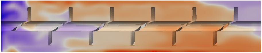
95 80 t = 0.5 s t=1s t=2s t=5s t = 10 s t = 15 s t = 20 s Figure 4.20: Predicted syngas mass fraction at different times and at statistically steadystate t = 20 s. Operation conditions are Treactor = 848 K, m biomass = 0.5 kg/h, N2 flow rate = 1.25 SLPM. t = 0.5 s t=1s t=2s t=5s t = 10 s t = 15 s t = 20 s Figure 4.21: Predicted tar mass fraction at different times and at statistically steadystate t = 20 s. Operation conditions are Treactor = 848 K, m biomass = 0.5 kg/h, N2 flow rate = 1.25 SLPM.