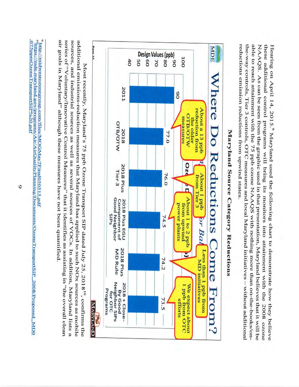
|
|
|
- Edgar Armstrong
- 5 years ago
- Views:
Transcription
1
2
3
4 EXHIBIT A
5
6
7
8
9
10
11
12

13

14
15

16
17

18
19
20

21

22
23
24
25
26

27

28

29
30
31
32
33
34 EXHIBIT B
35 Final Technical Support Document Good Neighbor Modeling Technical Support Document for 8-Hour Ozone State Implementation Plans Final Technical Support Document Prepared by: Alpine Geophysics, LLC 387 Pollard Mine Road Burnsville, NC June 2018 Project Number: TS-524
36 Final Technical Support Document Contents Page 1.0 INTRODUCTION Overview Study Background Purpose Overview of Modeling Approach Episode Selection Model Selection Base and Future Year Emissions Data Input Preparation and QA/QC Meteorology Input Preparation and QA/QC Initial and Boundary Conditions Development Air Quality Modeling Input Preparation and QA/QC Model Performance Evaluation Diagnostic Sensitivity Analyses MODEL SELECTION EPISODE SELECTION MODELING DOMAIN SELECTION Horizontal Domains Vertical Modeling Domain Data Availability Emissions Data Air Quality Meteorological Data Initial and Boundary Conditions Data MODEL INPUT PREPARATION PROCEDURES Meteorological Inputs WRF Model Science Configuration WRF Input Data Preparation Procedures WRF Model Performance Evaluation WRFCAMx/MCIP Reformatting Methodology Emission Inputs Available Emissions Inventory Datasets Development of CAMx-Ready Emission Inventories Episodic Biogenic Source Emissions 24 June Point Source Emissions Area and Non-Road Source Emissions Wildfires, Prescribed Burns, Agricultural Burns QA/QC and Emissions Merging 24 i
37 Final Technical Support Document Use of the Plume-in-Grid (PiG) Subgrid-Scale Plume Treatment Future-Year Emissions Modeling Photochemical Modeling Inputs CAMx Science Configuration and Input Configuration MODEL PERFORMANCE EVALUATION Model Performace Evaluation Overview of EPA Model Performance Evaluation Recommendations MPE Results FUTURE YEAR MODELING Future Year to be Simulated Future Year Growth and Controls Future Year Baseline Air Quality Simulations Identification of Future Nonattainment and Maintenance Receptors OZONE CONTRIBUTION MODELING Ozone contribution modeling Results SELECTED SIP REVISION APPROACHES Reliance upon alternative, equally credible, modeling data North American International Anthropogenic Contribution Relief from Additional Percentage of Boundary Conditions Alternate Significance Threshold Proportional Control by Contribution ( Red Lines ) Adressing Maintenance with 10 Year Emission Projection REFERENCES 44 June 2018 ii
38 Final Technical Support Document TABLES Table 1-1. EPA-identified eastern U.S. nonattainment and maintenance monitors. 8 Table 4-1. WRF and CAMx layers and their approximate height above ground level. 18 Table 4-2. Overview of routine ambient data monitoring networks. 20 Table 7-1. Alpine 4km Modeling-identified nonattainment monitors in the 4km domains. 30 Table 7-2. Alpine 4km Modeling-identified maintenance monitors in the 4km domains. 30 Table 7-3. Alpine 4km modeling-identified attainment monitors in the 4km domains previously identified by EPA as nonattainment or maintenance. 31 Table 8-1. Significant contribution (ppb) from region-specific anthropogenic emissions to 4km determined nonattainment monitor. 35 Table 8-2. Significant contribution (ppb) from region-specific anthropogenic emissions to 4km determined maintenance monitors. 35 Table 9-1. Alternate modeling results comparison for New York and Connecticut monitors. 37 Table 9-2. Harford, MD monitor ( ) design values for 2011 base case and two 2023 projection year scenarios with and without Canadian and Mexican contribution. 38 Table 9-3. International Contribution to Select Nonattainment Monitors and Anticipated Average Ozone Design Values (ppb) with Reasonable Proportion of Boundary Condition Relief. 39 Table 9-4. EPA 12km OSAT/APCA contributions to Texas nonattainment and maintenance monitors. 40 Table 9-5. Proportional contribution and reductions associated with significantly contributing upwind states to Harford, MD ( ) monitor in 4km modeling domain. 41 Table 9-6. Proportional contribution and reductions associated with significantly contributing upwind states to Brazoria, TX ( ) monitor in 12km modeling domain. 41 Table 9-7. Emission trend of annual anthropogenic NOx emissions (tons) for 1% linked states to Harford, MD monitor. 43 June 2018 iii
39 Final Technical Support Document FIGURES Figure 4-1. Map of 12km CAMx modeling domains. Source: EPA NAAQS NODA. 16 Figure 4-2. Maps of 4km CAMx modeling domains. Lake Michigan (left) and Mid- Atlantic (right). 17 Figure 5-1. Map of WRF domains. 22 Figure 8-1. OSAT regions for Mid-Atlantic 4km source contribution modeling. 33 June 2018 iv
40 1.0 INTRODUCTION Final Technical Support Document 1.1 OVERVIEW Sections 110(a)(1) and (2) of the Clean Air Act (CAA) require all states to adopt and submit to the U. S. Environmental Protection Agency (EPA) any revisions to their infrastructure State Implementation Plans (SIP) which provide for the implementation, maintenance and enforcement of a new or revised national ambient air quality standard (NAAQS). CAA section 110(a)(2)(D)(i)(I) requires each state to prohibit emissions that will significantly contribute to nonattainment of a NAAQS, or interfere with maintenance of a NAAQS, in a downwind state. The EPA revised the ozone NAAQS in March 2008 and completed the designation process to identify nonattainment areas in July Under this revision, the 8-hour ozone NAAQS form is the three year average of the fourth highest daily maximum 8-hour ozone concentrations with a threshold not to be exceeded of ppm (75 ppb). On October 1, 2015, EPA promulgated a revision to the ozone NAAQS, lowering the level of both the primary and secondary standards to 70 parts per billion (ppb) (80 FR 65292). Pursuant to CAA section 110(a), good neighbor SIPs are, therefore, due by October 1, This promulgated revision changed the threshold as to not exceed a value of ppm (70 ppb). This document serves to provide a technical support document for 4km air quality modeling and results recently conducted by Alpine Geophysics, LLC (Alpine) under contract to the Midwest Ozone Group (MOG) for purposes of individual state review and preparation of 8-hour ozone modeling analysis in support of revisions of the 2008 and hour ozone Good Neighbor State Implementation Plans (GNS). This document describes the overall modeling activities performed and results developed in order for a state to demonstrate whether they significantly contribute to nonattainment or interfere with maintenance of the 2008 or 2015 ozone NAAQS in a neighboring state. Our initial modeling effort was developed using EPA s national 12km modeling domain (12US2) and further refined with two 4km modeling domains over a Mid-Atlantic region and Lake Michigan. A comprehensive draft Modeling Protocol for the 12km 8-hour ozone SIP revision study was prepared and provided to EPA for comment and review. Based on EPA comments, the draft document was revised (Alpine, 2017a) to include many of the comments and recommendations submitted, most importantly, but not limited to, using EPA s 2023en modeling platform (EPA, 2017a). This 2023en modeling platform represents EPA s estimation of a projected base case that demonstrates compliance with final CSAPR update seasonal EGU NOx budgets. Our 4km modeling exercise largely utilized the same platform configuration with new meteorological data prepared for the 4km domains and 12km emissions nested to the 4km domains to support both attainment demonstration and source apportionment simulations. 1.2 STUDY BACKGROUND Section 110(a)(2)(D)(i)(I) of the CAA requires that states address the interstate transport of pollutants and ensure that emissions within the state do not contribute significantly to nonattainment in, or interfere with maintenance by, any other state. June
41 Final Technical Support Document On October 26, 2016, EPA published in the Federal Register (81 FR 74504) a final update to the Cross-State Air Pollution Rule (CSAPR) for the 2008 ozone NAAQS. In this final update, EPA outlines its four-tiered approach to addressing the interstate transport of pollution related to the ozone NAAQS, or states Good Neighbor responsibilities. EPA s approach determines which states contribute significantly to nonattainment areas or significantly interfere with air quality in maintenance areas in downwind states. EPA has determined that if a state s contribution to downwind air quality problems is below one percent of the applicable NAAQS, then it does not consider that state to be significantly contributing to the downwind area s nonattainment or maintenance concerns. EPA s approach to addressing interstate transport has been shaped by public notice and comment and refined in response to court decisions. As part of the final CSAPR update, EPA released regional air quality modeling to support the 2008 ozone NAAQS attainment date of 2017, indicating which states significantly contribute to nonattainment or maintenance area air quality problems in other states. To make these determinations, the EPA projected future ozone nonattainment and maintenance receptors, then conducted state-level ozone source apportionment modeling to determine which states contributed pollution over a pre-identified contribution threshold. A follow-up technical memorandum was issued by EPA on October 27, 2017 (Page, 2017) that provided supplemental information on interstate SIP submissions for the 2008 ozone NAAQS. In this memorandum, EPA provided future year 2023 design value calculations and source contribution results with updated modeling and included background on the four-step process interstate transport framework that the EPA uses to address the good neighbor provision for regional pollutants. This document also explains EPA s choice of 2023 as the new analytic year for the 2008 ozone NAAQS, introduced the no water approach to calculating relative response factors (RRFs) at coastal sites, and confirmed that there are no monitoring sites, outside of California, that were projected to have nonattainment or maintenance problems with respect to the 2008 ozone NAAQS of 75 ppb in Concurrent with EPA s modeling documented in the October 2017 memo, Alpine was conducting good neighbor SIP modeling for the Commonwealth of Kentucky (Alpine, 2017) using EPA s 2023en modeling platform. This analysis confirmed EPA s 3x3 grid cell findings and specifically noted that none of the problem monitors identified in EPA s final rule were predicted to be in nonattainment or have issues with maintenance in 2023 and therefore Kentucky (and by extension, any other upwind state) was not required to estimate its contribution to these monitors. On March 27, 2018, EPA released a technical memorandum (Tsirigotis, 2018) providing additional information on interstate SIP submissions for the 2015 ozone NAAQS. In this memo, EPA provided incremental results of their 12km modeling using a projection year of 2023, including updated source apportionment results, a no water grid cell RRF methodology, and a discussion of potential flexibilities in analytical approaches that an upwind state may consider in developing GNS. As discussed in greater detail in Section 1.3.3, the year of 2023 was selected as the analytic year in EPA s modeling primarily because it aligned with the anticipated June
42 Final Technical Support Document attainment year for Moderate ozone nonattainment areas and because it reflected the timeframe for implementing further emission reductions. EPA s goal in providing these new ozone air quality projections for 2023 was to assist states efforts to develop GNS for the 2015 ozone NAAQS. A number of monitors in the eastern U.S. were found to be in nonattainment of the 2015 ozone NAAQS with multiple states demonstrating contribution to projected downwind nonattainment area air quality over the one-percent threshold at EPA-identified nonattainment or maintenance monitors. These EPA-identified monitors are provided in Table 1-1 along with their current 3-yr design value for the period As EPA found that multiple state contributions to projected downwind maintenance problems at these monitors is above the one percent threshold and thus significant, additional analyses are required to identify these upwind state responsibilities under the Good Neighbor Provisions for the various ozone NAAQS. June
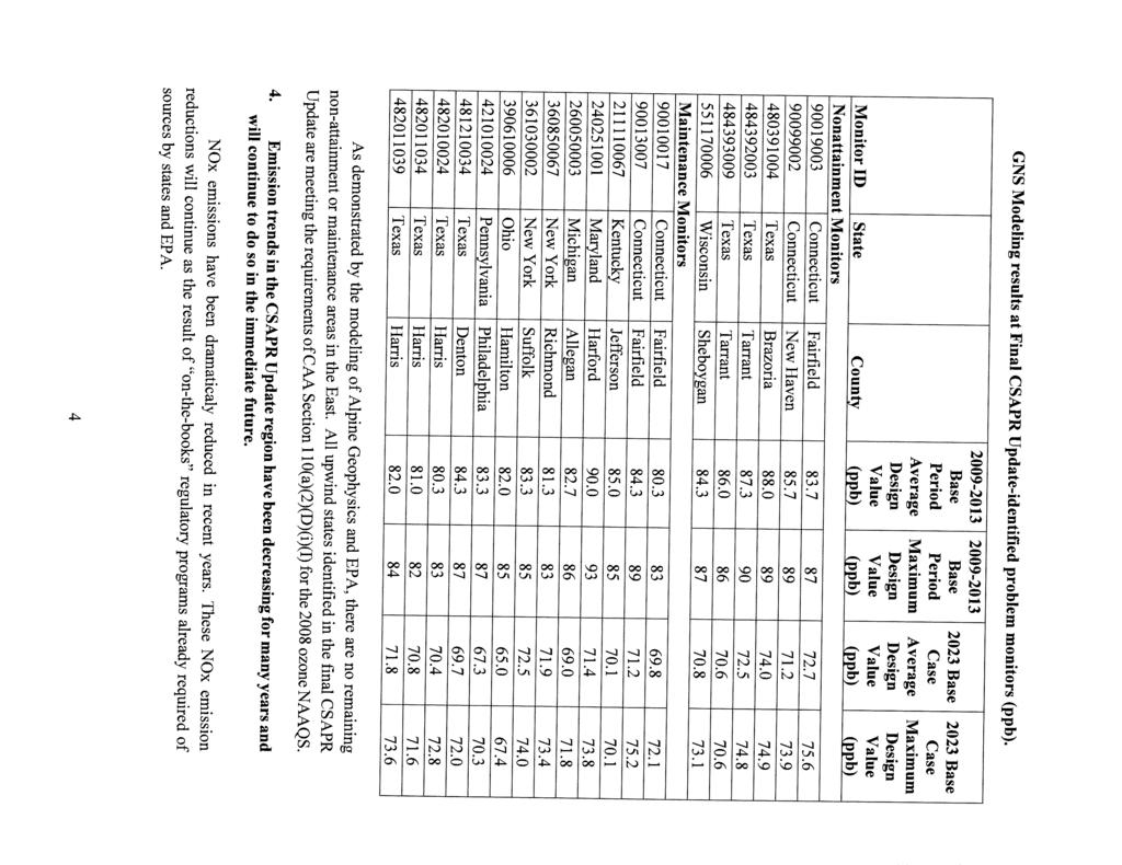
43 Final Technical Support Document Table 1-1. EPA-identified eastern U.S. nonattainment and maintenance monitors Avg Max 2023en 3x3 Avg 2023en 3x3 Max 2023en No Water Avg 2023en No Water Max Monitor State County CT Fairfield CT Fairfield CT Fairfield CT New Haven MD Harford MI Allegan MI Wayne NY Queens NY Richmond NY Suffolk TX Brazoria TX Denton TX Harris TX Harris TX Harris TX Tarrant WI Milwaukee WI Sheboygan Purpose This document primarily serves to provide the air quality modeling and source apportionment results for two 4km grid domains in support of revisions that states may make to their 2008 or hour ozone Good Neighbor State Implementation Plan (GNS). This document demonstrates that many of the eastern state receptors demonstrate modeled attainment using a finer grid 4km modeling domain (compared to 12km results). In addition, this document demonstrates the significance of international transport, that emissions activities within some states will not significantly contribute to nonattainment or interfere with maintenance of the 2008 or 2015 ozone NAAQS in a neighboring state, and that there may be options available to other states that do demonstrate significant contribution at air quality monitoring sites that qualify as nonattainment or maintenance. 1.3 OVERVIEW OF MODELING APPROACH The GNS 8-Hour ozone SIP modeling documented here includes an ozone simulation study using the 12 km grid based on EPA s 2023en modeling platform and preliminary source contribution assessment (EPA, 2016b) supplemented with two additional 4km modeling domains over the Mid-Atlantic region and Lake Michigan. June
44 Final Technical Support Document Episode Selection Episode selection is an important component of an 8-hour ozone attainment demonstration. EPA guidance recommends that 10 days be used to project 8-hour ozone Design Values at each critical monitor. The May 1 through August ozone season period was selected for the ozone SIP modeling primarily due to the following reasons: It is aligned with the 2011 NEI year, which is the latest NEI modeled in a regulatory platform. It is not an unusually low ozone year. Ambient meteorological and air quality data are available. A km CAMx modeling platform was available from the EPA that was leveraged for the GNS ozone SIP modeling. More details of the summer 2011 episode selection and justification using criteria in EPA s modeling guidance are contained in Section Model Selection Details on the rationale for model selection are provided in Section 2. The Weather Research Forecast (WRF) prognostic meteorological model was selected for the GNS ozone modeling using both the EPA 12US2 grid and two additional 4km modeling grids. Additional emission modeling was not required for the 12km simulation as the 2023en platform was provided to Alpine in pre-merged CAMx ready format. For the base and future year simulations without source apportionment, the 12km emissions were nested onto the 4km grid projections using the built in CAMx flexi-nesting capability. Flexi-nesting provides a computationally efficient framework to evenly divide the low level emissions from the 12km grid onto the nine (9) 4km grids. No flexi-nesting is necessary for elevated sources since the CAMx model injects elevated sources into the highest resolution grid for all domains. Emissions processing was completed by EPA for the 12km domain using the SMOKE emissions model for most source categories. The exceptions are that BEIS model was used for biogenic emissions and there are special processors for fires, windblown dust, lightning and sea salt emissions. The MOVES2014 on-road mobile source emissions model was used with SMOKE- MOVES to generate on-road mobile source emissions with EPA generated vehicle activity data provided in the NAAQS NODA. The CAMx photochemical grid model was also be used. The setup is based on the same WRF/SMOKE/BEIS/CAMx modeling system used in the EPA 2023en platform modeling. For the OSAT modeling, the 12km low level emissions were windowed onto the 4km domains using the standard CAMx WINDOW processor 1 as CAMx does not support flexi-nesting for source apportionment. 1 June
45 Final Technical Support Document Base and Future Year Emissions Data The 2023 future year was selected for the attainment demonstration modeling based on OAQPS Director Steven Page s October 27, 2017 memo (Page, 2017, page 4) to Regional Air Directors. In this memo, Director Page identified the two primary reasons the EPA selected 2023 for their 2008 NAAQS modeling; (1) the D.C. Circuit Court s response to North Carolina v. EPA in considering downwind attainment dates for the 2008 NAAQS, and (2) EPA s consideration of the timeframes that may be required for implementing further emission reductions as expeditiously as possible. The 2011 base case and 2023 future year emissions were based on EPA s en inventories with no adjustment. This platform has been identified by EPA as the base case for compliance with the final CSAPR update seasonal EGU NOx emission budgets Input Preparation and QA/QC Quality assurance (QA) and quality control (QC) of the emissions datasets are some of the most critical steps in performing air quality modeling studies. Because emissions processing is tedious, time consuming and involves complex manipulation of many different types of large databases, rigorous QA measures are a necessity to prevent errors in emissions processing from occurring. The GNS 8-Hour ozone modeling study utilized EPA s pre-qa/qc d emissions platform that followed a multistep emissions QA/QC approach for the 12km domain. Additional tabular and graphical review of the 4km emissions was conducted to ensure consistency with the 12km modeling results on spatial, temporal, and speciated levels Meteorology Input Preparation and QA/QC The CAMx km meteorological inputs are based on WRF meteorological modeling conducted by EPA. Details on the EPA 2011 WRF application and evaluation are provided by EPA (EPA 2014d). Additional WRF simulations were conducted to generate meteorological data fields to support the 4km modeling domains. A performance evaluation of this incremental modeling was prepared (Alpine, 2018a) and confirmed adequacy of the files for SIP attainment and contribution analyses Initial and Boundary Conditions Development Initial concentrations (IC) and Boundary Conditions (BC) are important inputs to the CAMx model. We ran 15 days of model spin-up before the first high ozone days occur in the modeling domain so the ICs are washed out of the modeling domain before the first high ozone day of the May-August 2011 modeling period. The lateral boundary and initial species concentrations are provided by a three dimensional global atmospheric chemistry model, GEOS-Chem (Yantosca, 2004) standard version with chemistry. The 4km domains were run as two-way interactive nests within the 12km simulation and therefore were provided with updated boundary conditions at each integration time step and provided up-scale feedback from the 4km domains to the 12km domain. June
46 Final Technical Support Document Air Quality Modeling Input Preparation and QA/QC Each step of the air quality modeling was subjected to QA/QC procedures. These procedures included verification of model configurations, confirmation that the correct data were used and processed correctly, and other procedures Model Performance Evaluation The Model Performance Evaluation (MPE) relied on the 12km CAMx MPE from EPA s associated modeling platforms. EPA s MPE recommendations in their ozone modeling guidance (EPA, 2007; 2014e) were followed in this evaluation. Many of EPA s MPE procedures have already been performed by EPA in their CAMx 2011 modeling database being used in the GNS ozone SIP modeling. An additional MPE was prepared by Alpine (Alpine, 2018b) to support the 4km domains and confirmed the adequacy of the analysis for SIP and contribution analyses Diagnostic Sensitivity Analyses Since no issues were identified in confirming Alpine s 12km CAMx runs compared to EPA s using the same modeling platform and configuration, additional diagnostic sensitivity analyses were not required. June
47 2.0 MODEL SELECTION Final Technical Support Document This section documents the models used in this 8-hour ozone GNS SIP modeling study. The selection methodology presented in this chapter mirrors EPA s and other s regulatory modeling in support of the 2008 Ozone NAAQS Preliminary Interstate Transport Assessment (Page, 2017; Alpine, 2017; EPA, 2016b) and technical memorandum providing additional information on the Interstate SIP submissions for the 2015 Ozone NAAQS (Tsirigotis, 2018). Unlike previous ozone modeling guidance that specified a particular ozone model (e.g., EPA, 1991 that specified the Urban Airshed Model; Morris and Myers, 1990), the EPA now recommends that models be selected for ozone SIP studies on a case-by-case basis. The latest EPA ozone guidance (EPA, 2014) explicitly mentions the CMAQ and CAMx PGMs as the most commonly used PGMs that would satisfy EPA s selection criteria but notes that this is not an exhaustive list and does not imply that they are preferred over other PGMs that could also be considered and used with appropriate justification. EPA s current modeling guidelines lists the following criteria for model selection (EPA, 2014e): It should not be proprietary; It should have received a scientific peer review; It should be appropriate for the specific application on a theoretical basis; It should be used with data bases which are available and adequate to support its application; It should be shown to have performed well in past modeling applications; It should be applied consistently with an established protocol on methods and procedures; It should have a user s guide and technical description; The availability of advanced features (e.g., probing tools or science algorithms) is desirable; and When other criteria are satisfied, resource considerations may be important and are a legitimate concern. For the GNS 8-hour ozone modeling, we used the WRF/SMOKE/MOVES2014/BEIS/CAMx/OSAT modeling system as the primary tool for demonstrating attainment of the ozone NAAQS at downwind monitors at downwind problem monitors. The utilized modeling system satisfies all of EPA s selection criteria. A description of the key models to be used in the GNS ozone SIP modeling follows. WRF/ARW: The Weather Research and Forecasting (WRF) 2 Model is a mesoscale numerical weather prediction system designed to serve both operational forecasting and atmospheric research needs (Skamarock, 2004; 2006; Skamarock et al., 2005). The Advanced Research WRF (ARW) version of WRF was used in this ozone modeling study. It features multiple dynamical cores, a 3-dimensional variational (3DVAR) data assimilation system, and a software architecture allowing for computational parallelism and system extensibility. WRF is suitable 2 June
48 Final Technical Support Document for a broad spectrum of applications across scales ranging from meters to thousands of kilometers. The effort to develop WRF has been a collaborative partnership, principally among the National Center for Atmospheric Research (NCAR), the National Oceanic and Atmospheric Administration (NOAA), the National Centers for Environmental Prediction (NCEP) and the Forecast Systems Laboratory (FSL), the Air Force Weather Agency (AFWA), the Naval Research Laboratory, the University of Oklahoma, and the Federal Aviation Administration (FAA). WRF allows researchers the ability to conduct simulations reflecting either real data or idealized configurations. WRF provides operational forecasting a model that is flexible and efficient computationally, while offering the advances in physics, numerics, and data assimilation contributed by the research community. SMOKE: The Sparse Matrix Operator Kernel Emissions (SMOKE) 3 modeling system is an emissions modeling system that generates hourly gridded speciated emission inputs of mobile, non-road, area, point, fire and biogenic emission sources for photochemical grid models (Coats, 1995; Houyoux and Vukovich, 1999). As with most emissions models, SMOKE is principally an emission processing system and not a true emissions modeling system in which emissions estimates are simulated from first principles. This means that, with the exception of mobile and biogenic sources, its purpose is to provide an efficient, modern tool for converting an existing base emissions inventory data into the hourly gridded speciated formatted emission files required by a photochemical grid model. SMOKE was used by EPA to prepare 2023en emission inputs for non-road mobile, area and point sources. These files were adopted and used as-is for this analysis. SMOKE-MOVES: SMOKE-MOVES uses an Emissions Factor (EF) Look-Up Table from MOVES, gridded vehicle miles travelled (VMT) and other activity data and hourly gridded meteorological data (typically from WRF) and generates hourly gridded speciated on-road mobile source emissions inputs. MOVES2014: MOVES is EPA s latest on-road mobile source emissions model that was first released in July 2014 (EPA, 2014a,b,c). MOVES2014 includes the latest on-road mobile source emissions factor information. Emission factors developed by EPA were used in this analysis. BEIS: Biogenic emissions were modeled by EPA using version 3.61 of the Biogenic Emission Inventory System (BEIS). First developed in 1988, BEIS estimates volatile organic compound (VOC) emissions from vegetation and nitric oxide (NO) emissions from soils. Because of resource limitations, recent BEIS development has been restricted to versions that are built within the Sparse Matrix Operational Kernel Emissions (SMOKE) system. CAMx: The Comprehensive Air quality Model with Extensions (CAMx 5 ) is a state-of-science One-Atmosphere photochemical grid model capable of addressing ozone, particulate matter (PM), visibility and acid deposition at regional scale for periods up to one year (ENVIRON, June
49 Final Technical Support Document ). CAMx is a publicly available open-source computer modeling system for the integrated assessment of gaseous and particulate air pollution. Built on today s understanding that air quality issues are complex, interrelated, and reach beyond the urban scale, CAMx is designed to (a) simulate air quality over many geographic scales, (b) treat a wide variety of inert and chemically active pollutants including ozone, inorganic and organic PM 2.5 and PM 10 and mercury and toxics, (c) provide source-receptor, sensitivity, and process analyses and (d) be computationally efficient and easy to use. The U.S. EPA has approved the use of CAMx for numerous ozone and PM State Implementation Plans throughout the U.S., and has used this model to evaluate regional mitigation strategies including those for most recent regional rules (e.g., Transport Rule, CAIR, NO X SIP Call, etc.). CAMx Version 6.40 was used in this study. OSAT: The Ozone Source Apportionment Technique (OSAT) tool of CAMx was selected to develop source contribution and significant contribution calculations and was applied for this analysis. SMAT-CE: The Software for the Modeled Attainment Test - Community Edition (SMAT-CE) 7 is a PC-based software tool that can perform the modeled attainment tests for particulate matter and ozone, and calculate changes in visibility at Class I areas as part of the reasonable progress analysis for regional haze. Version 1.2 (Beta) was used in this analysis June
50 3.0 EPISODE SELECTION Final Technical Support Document EPA s most recent 8-hour ozone modeling guidance (EPA, 2014e) contains recommended procedures for selecting modeling episodes The GNS ozone SIP revision modeling used the May through end of August 2011 modeling period because it satisfies the most criteria in EPA s modeling guidance episode selection discussion. EPA guidance recommends that 10 days be used to project 8-hour ozone Design Values at each critical monitor. The May through August 2011 period has been selected for the ozone SIP modeling primarily due to being aligned with the 2011 NEI year, not being an unusually low ozone year and availability of a km CAMx modeling platform from the EPA NAAQS NODA. June

51 4.0 MODELING DOMAIN SELECTION Final Technical Support Document This section summarizes the modeling domain definitions for the GNS 8-hour ozone modeling, including the domain coverage, resolution, and map projection. It also discusses emissions, aerometric, and other data available for use in model input preparation and performance testing. 4.1 HORIZONTAL DOMAINS The GNS ozone SIP modeling used a 12 km continental U.S. (12US2) domain and two 4 km subnested domains; one over the Mid-Atlantic region and another over Lake Michigan and surrounding states. The 12 km nested grid modeling domain configuration is shown in Figure 4-1 with the two 4km domains represented in Figure 4-2. The 12 km domain shown in Figure 4-1 represents the CAMx 12km air quality and SMOKE/BEIS emissions modeling domain. The WRF meteorological modeling was run on larger 12 km modeling domains than used for CAMx as demonstrated in EPA s meteorological model performance evaluation document (EPA, 2014d). The WRF meteorological modeling domains are defined larger than the air quality modeling domains because meteorological models can sometimes produce artifacts in the meteorological variables near the boundaries as the prescribed boundary conditions come into dynamic balance with the coupled equations and numerical methods in the meteorological model. Figure 4-1. Map of 12km CAMx modeling domains. Source: EPA NAAQS NODA. June
52 Final Technical Support Document Figure 4-2. Maps of 4km CAMx modeling domains. Lake Michigan (left) and Mid-Atlantic (right). 4.2 VERTICAL MODELING DOMAIN The CAMx vertical structure is primarily defined by the vertical layers used in the WRF meteorological modeling. The WRF model employs a terrain following coordinate system defined by pressure, using multiple layer interfaces that extend from the surface to 50 mb (approximately 19 km above sea level). EPA ran WRF using 35 vertical layers. A layer averaging scheme is adopted for CAMx simulations whereby multiple WRF layers are combined into one CAMx layer to reduce the air quality model computational time. Table 4-1 displays the approach for collapsing the WRF 35 vertical layers to 25 vertical layers in CAMx for the 12km and 4km grid domains. June
53 Final Technical Support Document Table 4-1. WRF and CAMx layers and their approximate height above ground level. CAMx Layer Approx. Height (m AGL) WRF Layers Sigma P Pressure (mb) , , , , , , , , , , , , , , , , , , , , , June
54 Final Technical Support Document 4.3 DATA AVAILABILITY The CAMx modeling systems requires emissions, meteorology, surface characteristics, initial and boundary conditions (IC/BC), and ozone column data for defining the inputs Emissions Data Without exception, the 2011 base year and 2023 base case emissions inventories for ozone modeling for this analysis were based on emissions obtained from the EPA s en modeling platform. This platform was obtained from EPA, via LADCO, in late September of 2017 and represents EPA s best estimate of all promulgated national, regional, and local control strategies, including final implementation of the seasonal EGU NOx emission budgets outlined in CSAPR Air Quality Data from ambient monitoring networks for gas species are used in the model performance evaluation. Table 4-2 summarizes routine ambient gaseous and PM monitoring networks available in the U.S Meteorological Data The 12km meteorological data were generated by EPA using the WRF prognostic meteorological model (EPA, 2014d). Alpine ran WRF with identical physics options and configuration for the 4km domains as was run by EPA for the 12km domain. WRF was run on a continental U.S. 12 km grid for the NAAQS NODA platform and for two subnested 4km domains as described in earlier sections Initial and Boundary Conditions Data The lateral boundary and initial species concentrations are provided by a three dimensional global atmospheric chemistry model, GEOS-Chem (Yantosca, 2004) standard version with chemistry. The global GEOS-Chem model simulates atmospheric chemical and physical processes driven by assimilated meteorological observations from the NASA s Goddard Earth Observing System (GEOS-5; additional information available at: and This model was run for 2011 with a grid resolution of 2.0 degrees x 2.5 degrees (latitude-longitude). The predictions were used to provide one-way dynamic boundary concentrations at one-hour intervals and an initial concentration field for the CAMx simulations. The 2011 boundary concentrations from GEOS-Chem will be used for the 2011 and 2023 model simulations. The 4km domains were run as two-way interactive nests within the 12km simulation and therefore provided with updated boundary conditions at each integration time step and provided up-scale feedback from the 4km domains to the 12km domain. June
55 Final Technical Support Document Table 4-2. Overview of routine ambient data monitoring networks. Monitoring Network Chemical Species Measured Sampling Period Data Availability/Source The Interagency Monitoring of Protected Visual Environments (IMPROVE) Clean Air Status and Trends Network (CASTNET) National Atmospheric Deposition Program (NADP) Air Quality System (AQS) or Aerometric Information Retrieval Speciated PM25 and PM10 (see species mappings) 1 in 3 days; 24 hr average Speciated PM25, Ozone (see species mappings) Approximately 1- week average Wet deposition (hydrogen (acidity as ph), sulfate, nitrate, ammonium, chloride, and base cations (such as calcium, magnesium, potassium and sodium)), Mercury 1-week average CO, NO2, O3, SO2, PM25, PM10, Pb Typically hourly average System (AIRS) Chemical Speciation Network (CSN) Speciated PM 24-hour average Photochemical Assessment Monitoring Stations (PAMS) National Park Service Gaseous Pollutant Monitoring Network Varies for each of 4 station types. Acid deposition (Dry; SO4, NO3, HNO3, NH4, SO2), O3, meteorological data Hourly June
56 Final Technical Support Document 5.0 MODEL INPUT PREPARATION PROCEDURES This section summarizes the procedures used in developing the meteorological, emissions, and air quality inputs to the CAMx model for the GNS 8-hour ozone modeling on the 12 km and 4 km grids for the May through August 2011 period. Both the 12 km and 4 km CAMx modeling databases are based on the EPA en platform (EPA, 2017a; Page, 2017) databases. While some of the data prepared by EPA for this platform are new, many of the files are largely based on the NAAQS NODA platform. More details on the NAAQS NODA 2011 CAMx database development are provided in EPA documentation as follows: Technical Support Document (TSD) Preparation of Emissions Inventories for the Version 6.3, 2011 Emissions Modeling Platform (EPA, 2016a). Meteorological Model Performance for Annual 2011 WRF v3.4 Simulation (EPA, 2014d). Air Quality Modeling Technical Support Document for the 2015 Ozone NAAQS Preliminary Interstate Transport Assessment (EPA, 2016b). The modeling procedures used in the modeling are consistent with over 20 years of EPA ozone modeling guidance documents (e.g., EPA, 1991; 1999; 2005a; 2007; 2014), other recent 8-hour ozone modeling studies conducted for various State and local agencies using these or other state-of-science modeling tools (see, for example, Morris et al., 2004a,b, 2005a,b; 2007; 2008a,b,c; Tesche et al., 2005a,b; Stoeckenius et al., 2009; ENVIRON, Alpine and UNC, 2013; Adelman, Shanker, Yang and Morris, 2014; 2015), as well as the methods used by EPA in support of the recent Transport analysis (EPA, 2010; 2015b, 2016b). 5.1 METEOROLOGICAL INPUTS WRF Model Science Configuration For the 12km domain, Version 3.4 of the WRF model, Advanced Research WRF (ARW) core (Skamarock, 2008) was used for generating the 2011 simulations. Selected physics options include Pleim-Xiu land surface model, Asymmetric Convective Model version 2 planetary boundary layer scheme, KainFritsch cumulus parameterization utilizing the moisture-advection trigger (Ma and Tan, 2009), Morrison double moment microphysics, and RRTMG longwave and shortwave radiation schemes (Gilliam and Pleim, 2010). The WRF model configuration was prepared by EPA (EPA, 2014d). The 4km domains were prepared using a nested WRF 3.9 simulation with domains shown in Figure 5-1. This domain, a 36km continental domain and a 12km domain that extends from the western border of the Dakotas off the eastern seaboard has two focused 4km domains over Lake Michigan and the Mid-Atlantic states. The WRF configuration options used in the 4km simulation were the same as those used by EPA, with the exception that no cumulus parameterization was used on the 4km domains. A summary of the 4km WRF application and evaluation are presented elsewhere (Alpine, 2018a). June 2018
57 Final Technical Support Document Figure 5-1. Map of WRF domains. The outer domain is the 36km CONUS domain, the large domain is the 12km domain and the inner are the Lake Michigan (left) and Mid-Atlantic (right) 4km domains WRF Input Data Preparation Procedures For the 4km domain a summary of the WRF input data preparation procedures that were used are listed in EPA s documentation (EPA, 2014d). A summary of the 4km WRF application and evaluation are presented elsewhere (Alpine, 2018a) WRF Model Performance Evaluation The WRF model evaluation approach was based on a combination of qualitative and quantitative analyses. The quantitative analysis was divided into monthly summaries of 2-m temperature, 2-m mixing ratio, and 10-m wind speed using the boreal seasons to help generalize the model bias and error relative to a set of standard model performance benchmarks. The qualitative approach was to compare spatial plots of model estimated monthly total precipitation with the monthly PRISM precipitation. The WRF model performance evaluation for the 12km domain is provided in EPA s documentation (EPA, 2014d). A separate MPE for the 4km WRF simulations was prepared by Alpine (Alpine, 2018a). This evaluation is comprised of a quantitative and qualitative evaluation of WRF generated fields. The quantitative model performance evaluation of WRF using surface meteorological June
58 Final Technical Support Document measurements was performed using the publicly available METSTAT 8 evaluation tool. METSTAT calculates statistical performance metrics for bias, error and correlation for surface winds, temperature and mixing ratio and can produce time series of predicted and observed meteorological variables and performance statistics. Alpine also conducted a qualitative comparison of WRF estimated precipitation with the Climate Prediction Center (CPC) retrospective analysis data WRFCAMx/MCIP Reformatting Methodology The WRF meteorological model output data was processed to provide inputs for the CAMx photochemical grid model. The WRFCAMx processor maps WRF meteorological fields to the format required by CAMx. It also calculates turbulent vertical exchange coefficients (Kv) that define the rate and depth of vertical mixing in CAMx. The methodology used by EPA to reform the meteorological data into CAMx format is provided in documentation provided with the wrfcamx conversion utility. The meteorological data generated by the WRF simulations were processed by EPA using WRFCAMx v4.3 (Ramboll Environ, 2014) meteorological data processing program to create model-ready meteorological inputs to CAMx. The 4km domains were processed using WRFCAMx v In running WRFCAMx, vertical eddy diffusivities (Kv) were calculated using the Yonsei University (YSU) (Hong and Dudhia, 2006) mixing scheme with a minimum Kv of 0.1 m2/sec except for urban grid cells where the minimum Kv was reset to 1.0 m2/sec within the lowest 200 m of the surface in order to enhance mixing associated with the night time urban heat island effect. In addition, all domains used the subgrid convection and subgrid stratoform stratiform cloud options in our wrfcamx. 5.2 EMISSION INPUTS Available Emissions Inventory Datasets EPA s 2011 base year and 2023 future year emission inventories from the en modeling platform (EPA, 2017a) were used for all categories without exception Development of CAMx-Ready Emission Inventories CAMx-ready emission inputs were generated by EPA mainly by the SMOKE and BEIS emissions models. CAMx requires two emission input files for each day: (1) low level gridded emissions that are emitted directly into the first layer of the model from sources at the surface with little or no plume rise; and (2) elevated point sources (stacks) with plume rise calculated from stack parameters and meteorological conditions. For this analysis, CAMx was operated using version 6 revision 4 of the Carbon Bond chemical mechanism (CB6r4). Additional emission modeling was not required for the 12km simulation as the 2023en platform was provided to Alpine in pre-merged CAMx ready format. For the base and future year simulations without source apportionment, the 12km emissions were nested onto the 4km grid projections using the built in CAMx flexi-nesting capability. Flexi-nesting provides a June
59 Final Technical Support Document computationally efficient framework to evenly divide the low level emissions from the 12km grid onto the nine (9) 4km grids. No flexi-nesting is necessary for elevated sources since the CAMx model injects elevated sources into the highest resolution grid for all domains Episodic Biogenic Source Emissions Biogenic emissions were generated by EPA using the BEIS biogenic emissions model within SMOKE. BEIS uses high resolution GIS data on plant types and biomass loadings and the WRF surface temperature fields, and solar radiation (modeled or satellite-derived) to develop hourly emissions for biogenic species on the 12 km grids. BEIS generates gridded, speciated, temporally allocated emission files Point Source Emissions 2011 point source emissions were from the 2011 en modeling platform. Point sources were developed in two categories: (1) major point sources with Continuous Emissions Monitoring (CEM) devices; and (2) point sources without CEMs. For point sources with continuous emissions monitoring (CEM) data, day-specific hourly NOX and SO2 emissions were used for the 2011 base case emissions scenario. The VOC, CO and PM emissions for point sources with CEM data were based on the annual emissions temporally allocated to each hour of the year using the CEM hourly heat input. The locations of the point sources were converted to the LCP coordinate system used in the modeling. They were processed by EPA using SMOKE to generate the temporally varying (i.e., day-of-week and hour-of-day) speciated emissions needed by CAMx, using profiles by source category from the EPA en modeling platform Area and Non-Road Source Emissions 2011 area and non-road emissions were from the 2011 en modeling platform. The area and non-road sources were spatially allocated to the grid using an appropriate surrogate distribution (e.g., population for home heating, etc.). The area sources were temporally allocated by month and by hour of day using the EPA source-specific temporal allocation factors. The SMOKE source-specific CB6 speciation allocation profiles were also used Wildfires, Prescribed Burns, Agricultural Burns Fire emissions in 2011NEIv2 were developed based on Version 2 of the Satellite Mapping Automated Reanalysis Tool for Fire Incident Reconciliation (SMARTFIRE) system (Sullivan, et al., 2008). SMARTFIRE2 was the first version of SMARTFIRE to assign all fires as either prescribed burning or wildfire categories. In past inventories, a significant number of fires were published as unclassified, which impacted the emissions values and diurnal emissions pattern. Recent updates to SMARTFIRE include improved emission factors for prescribed burning QA/QC and Emissions Merging EPA processed the emissions by major source category in several different streams, including area sources, on-road mobile sources, non-road mobile sources, biogenic sources, non-cem point sources, CEM point sources using day-specific hourly emissions, and emissions from fires. Separate Quality Assurance (QA) and Quality Control (QC) were performed for each stream of emissions processing and in each step following the procedures utilized by EPA. SMOKE June
60 Final Technical Support Document includes advanced quality assurance features that include error logs when emissions are dropped or added. In addition, we generated visual displays that included spatial plots of the hourly emissions for each major species (e.g., NOX, VOC, some speciated VOC, SO2, NH3, PM and CO). Scripts to perform the emissions merging of the appropriate biogenic, on-road, non-road, area, low-level, fire, and point emission files were written to generate the CAMx-ready twodimensional day and domain-specific hourly speciated gridded emission inputs. The point source and, as available elevated fire, emissions were processed into the day-specific hourly speciated emissions in the CAMx-ready point source format. The resultant CAMx model-ready emissions were subjected to a final QA using spatial maps to assure that: (1) the emissions were merged properly; (2) CAMx inputs contain the same total emissions; and (3) to provide additional QA/QC information Use of the Plume-in-Grid (PiG) Subgrid-Scale Plume Treatment Consistent with the EPA 2011 modeling platform, no PiG subgrid-scale plume treatment will be used Future-Year Emissions Modeling Future-year emission inputs were generated by processing the 2023 emissions data provided with EPA s en modeling platform without exception. 5.3 PHOTOCHEMICAL MODELING INPUTS CAMx Science Configuration and Input Configuration Version of CAMx (Version 6.40) was used in the GNS ozone modeling. The CAMx model setup used is defined by EPA in its air quality modeling technical support document (EPA, 2016b, 2017). June
61 Final Technical Support Document 6.0 MODEL PERFORMANCE EVALUATION The CAMx 2011 base case model estimates are compared against the observed ambient ozone and other concentrations to establish that the model is capable of reproducing the current year observed concentrations so it is likely a reliable tool for estimating future year ozone levels. 6.1 MODEL PERFORMACE EVALUATION Overview of EPA Model Performance Evaluation Recommendations EPA current (EPA, 2007) and draft (EPA, 2014e) ozone modeling guidance recommendations for model performance evaluation (MPE) describes a MPE framework that has four components: Operation evaluation that includes statistical and graphical analysis aimed at determining how well the model simulates observed concentrations (i.e., does the model get the right answer). Diagnostic evaluation that focuses on process-oriented evaluation and whether the model simulates the important processes for the air quality problem being studied (i.e., does the model get the right answer for the right reason). Dynamic evaluation that assess the ability of the model air quality predictions to correctly respond to changes in emissions and meteorology. Probabilistic evaluation that assess the level of confidence in the model predictions through techniques such as ensemble model simulations. EPA s guidance recommends that At a minimum, a model used in an attainment demonstration should include a complete operational MPE using all available ambient monitoring data for the base case model simulations period (EPA, 2014, pg. 63). And goes on to say Where practical, the MPE should also include some level of diagnostic evaluation. EPA notes that there is no single definite test for evaluation model performance, but instead there are a series of statistical and graphical MPE elements to examine model performance in as many ways as possible while building a weight of evidence (WOE) that the model is performing sufficiently well for the air quality problem being studied MPE Results Because this 2011 ozone modeling is using a CAMx 2011 modeling database developed by EPA, we include by reference the air quality modeling performance evaluation as conducted by EPA (EPA, 2016b) on the national 12km domain. Alpine additionally conducted an MPE on the 4km domains (Alpine, 2018b) that generated results consistent with the 12km simulation and configuration. In summary, EPA conducted an operational model performance evaluation for ozone to examine the ability of the CAMx v6.32 and v.6.40 modeling systems to simulate 2011 measured concentrations. This evaluation focused on graphical analyses and statistical metrics of model predictions versus observations. Details on the evaluation methodology, the calculation of performance statistics, and results are provided in Appendix A of that report. June
62 Final Technical Support Document Overall, the ozone model performance statistics for the CAMx v simulation are similar to those from the CAMx v simulation performed by EPA for the final CSAPR Update. The 2011 CAMx model performance statistics are within or close to the ranges found in other recent peer-reviewed applications (Simon et al, 2012). As described in Appendix A of the AQ TSD, the predictions from the 2011 modeling platform correspond closely to observed concentrations in terms of the magnitude, temporal fluctuations, and geographic differences for 8-hour daily maximum ozone. Alpine conducted a separate operational model performance evaluation for the two 4km modeling domains (Alpine, 2018b) and found that 4km domains for the 2011en platform performed similarly to EPA s 12km MPE that fell within or close to the ranges found in other recent peer-reviewed applications (Simon et al, 2012). Thus, the model performance results demonstrate the scientific credibility of the two 4km domains using the 2011 modeling platform chosen and used for this analysis. These results provide confidence in the ability of the modeling platform to provide a reasonable projection of expected future year ozone concentrations and contributions over the two 4km grids. June
63 7.0 FUTURE YEAR MODELING Final Technical Support Document This chapter discusses the future year modeling used in the GNS 8-hour ozone modeling effort. 7.1 FUTURE YEAR TO BE SIMULATED As discussed in Section 1, to support the 2008 and 2015 ozone NAAQS preliminary interstate transport assessment, EPA conducted air quality modeling to project ozone concentrations at individual monitoring sites to 2023 and to estimate state-by-state contributions to those 2023 concentrations. The projected 2023 ozone concentrations were used to identify ozone monitoring sites that are projected to be nonattainment or have maintenance problems for the two ozone NAAQS in 2023 and for which upwind states have been identified as significant contributors. 7.2 FUTURE YEAR GROWTH AND CONTROLS In September 2017, EPA released the revised en modeling platform that was the source for the 2023 future year emissions in this analysis. This platform has been identified by EPA as the base case for compliance with the final CSAPR update seasonal EGU NOx emission budgets. Additionally, there were several emission categories and model inputs/options that were held constant at 2011 levels as follows: Biogenic emissions. Wildfires, Prescribed Burns and Agricultural Burning (open land fires). Windblown dust emissions. Sea Salt. 36 km CONUS domain Boundary Conditions (BCs) km meteorological conditions. All model options and inputs other than emissions. The effects of climate change on the future year meteorological conditions were not accounted. It has been argued that global warming could increase ozone due to higher temperatures producing more biogenic VOC and faster photochemical reactions (the so called climate penalty). However, the effects of inter-annual variability in meteorological conditions will be more important than climate change given the 12 year difference between the base (2011) and future (2023) years. It has also been noted that the level of ozone being transported into the U.S. from Asia has also increased. 7.3 FUTURE YEAR BASELINE AIR QUALITY SIMULATIONS A 2023 future year base case CAMx simulation was conducted and 2023 ozone design value projection calculations were made based on EPA s latest ozone modeling guidance (EPA, 2014e) for the 12US2 and two 4km modeling domains in this analysis Identification of Future Nonattainment and Maintenance Receptors The ozone predictions from the 2011 and 2023 CAMx model simulations were used to project average and maximum ozone design values to 2023 following the approach described in the EPA s draft guidance for attainment demonstration modeling (US EPA, June
64 Final Technical Support Document 2014b). Using the approach in the final CSAPR Update, we evaluated the 2023 projected average and maximum design values in conjunction with the most recent measured ozone design values (i.e., ) to identify sites that may warrant further consideration as potential nonattainment or maintenance sites in If the approach in the CSAPR Update is applied to evaluate the projected design values, those sites with 2023 average design values that exceed the NAAQS (i.e., 2023 average design values of 71 ppb or greater) and that are currently measuring nonattainment would be considered to be nonattainment receptors in Similarly, with the CSAPR Update approach, monitoring sites with a projected 2023 maximum design value that exceeds the NAAQS would be projected to be maintenance receptors in In the CSAPR Update approach, maintenance-only receptors include both those monitoring sites where the projected 2023 average design value is below the NAAQS, but the maximum design value is above the NAAQS, and monitoring sites with projected 2023 average design values that exceed the NAAQS, but for which current design values based on measured data do not exceed the NAAQS. As documented in EPA s March 2018 technical memorandum (Tsirigotis, 2018), EPA used results of CAMx v6.40 to model emissions in 2011 and 2023 to project base period average and maximum ozone design values to 2023 at monitoring sites nationwide. In projecting these future year design values, EPA applied its own modeling guidance, which recommends using model predictions from the 3x3 array of grid cells surrounding the location of the monitoring site. In response to comments submitted on the January 2017 NODA and other analyses, EPA also projected 2023 design values based on a modified version of the 3x3 approach for those monitoring sites located in coastal areas (Tsirigotis, 2018). This modeling was intended as an alternate approach to addressing complex meteorological monitor locations without having to rerun the simulations on finer grid scales. Alpine s applied approach in developing and using 4km grid domains further followed EPA s guidance recommendation that grid resolution finer than 12 km would generally be more appropriate for areas with a combination of complex meteorology, strong gradients in emissions sources, and/or land-water interfaces in or near the nonattainment area(s). (EPA, 2014e) We used the finer grid resolution and the Software for the Modeled Attainment Test - Community Edition 10 (SMAT-CE) tool consistent with EPA s 12km attainment demonstration modeling methods calculating relative response factors and 3x3 neighborhoods (EPA, 2014e). Alpine also prepared 2023 projected average and maximum design values in conjunction with the most recent measured ozone design values ( ) to identify sites in these 4km domains that may warrant further consideration as potential nonattainment or maintenance sites in After applying the approach outlined in the final CSAPR update (and described above) to evaluate the projected design values from the 4km analysis, we developed a list of nonattainment and maintenance monitors located within these two eastern 4km domains resulting from the approach. Modeled nonattainment monitors defined using Alpine s 4km 10 June
65 Final Technical Support Document simulation are provided in Table 7-1 along with their calculated 2023 average and maximum design values from both EPA s no water calculation approach and Alpine s 4km simulation and most current design values. Similarly, Table 7-2 presents the modeled maintenance monitors with their calculated average and maximum design values from both simulations and the most current design value data. Monitors originally designated as nonattainment or maintenance by EPA using their no water calculation and found to be neither nonattainment or maintenance using Alpine s 4km modeling are presented in Table 7-3. A full list of monitor locations and modeled average and maximum ozone design values for the 4km domain modeling is provided in Appendix A of this report. Table 7-1. Alpine 4km Modeling-identified nonattainment monitors in the 4km domains. Monitor State County DVb (2011) MD Harford WI Sheboygan Table 7-2. Alpine 4km Modeling-identified maintenance monitors in the 4km domains. Monitor State County DVb (2011) Ozone Design Value (ppb) EPA "No Water" Alpine 12km Modeling 4km Modeling DVf (2023) Ave DVf (2023) Max DVf (2023) Ave DVf (2023) Max Ozone Design Value (ppb) EPA "No Water" 12km Modeling Alpine 4km Modeling DVf (2023) Ave DVf (2023) Max DVf (2023) Ave DVf (2023) Max 2016 DV DV CT Fairfield CT Fairfield CT Fairfield CT New Haven CT New London MI Allegan NJ Gloucester NY Richmond NY Suffolk PA Philadelphia June
66 Final Technical Support Document Table 7-3. Alpine 4km modeling-identified attainment monitors in the 4km domains previously identified by EPA as nonattainment or maintenance. Ozone Design Value (ppb) EPA "No Water" 12km Modeling Alpine 4km Modeling Monitor State County DVb (2011) DVf (2023) Ave DVf (2023) Max DVf (2023) Ave DVf (2023) Max 2016 DV NY Queens WI Milwaukee The procedures for calculating projected 2023 average and maximum design values are described in Section 3.2 of EPA s air quality technical support document (EPA, 2016b). The only noted differences are that Alpine used 4km modeling results, compared to EPA s 12km, and did not remove no water cells from the calculation as further described in the March 2018 memorandum. June
67 8.0 OZONE CONTRIBUTION MODELING Final Technical Support Document Alpine further performed region, source category-level ozone source apportionment modeling using the CAMx Ozone Source Apportionment Technology (OSAT) technique to provide information regarding the expected contribution of 2023 base case NOx and VOC emissions from each category within each region to projected 2023 concentrations at downwind air quality monitors. This OSAT modeling was conducted for the Mid-Atlantic 4km region but not the Lake Michigan 4km domain. In the source apportionment model run, we tracked the ozone formed from each of the following contribution categories (i.e., tags): EGUs NOx and VOC emissions from each region tracked individually from electric generating units (EGUs); Non-EGU Point Sources - NOx and VOC emissions from each region tracked individually from elevated source non-egu point sources; Nonroad - NOx and VOC emissions from each region tracked individually nonroad mobile, marine, aircraft, and railroad sources; Area - NOx and VOC emissions from each region tracked individually from non-point stationary sources; Onroad - NOx and VOC emissions from each region tracked individually from onroad mobile sources; Biogenics - biogenic NOX and VOC emissions from each region; Boundary Concentrations concentrations transported into the modeling domain from the lateral boundaries; Canada and Mexico NOx and VOC anthropogenic emissions from sources in the portions of Canada and Mexico included in the modeling domain (contributions from each country were not modeled separately; both are included as a single tag); Fires combined emissions from wild and prescribed fires domain-wide (i.e., not by individual region); and Offshore combined emissions from offshore marine vessels and offshore drilling platforms (i.e., not by individual region). The contribution modeling conducted for this analysis provided contribution to ozone from source regions, informed by MOG s 12km OSAT modeling and displayed in Figure 8-1, for each noted source category individually. In contrast to EPA s contribution modeling using the OSAT/Anthropogenic Precursor Culpability Analysis (APCA) technique, Alpine s OSAT technique assigns ozone formed from biogenic VOC and NOx emissions that reacts with anthropogenic NOx and VOC to the biogenic category. EPA s technique of using OSAT/APCA assigns to the anthropogenic emission total the combined ozone formed from reactions between biogenic VOC and NOx with anthropogenic NOx and VOC. Alpine s position on the selection of the OSAT technique has been documented elsewhere ossstateairpollutionrulemodelingplatform.pdf June

68 Final Technical Support Document Figure 8-1. OSAT regions for Mid-Atlantic 4km source contribution modeling. Consistent with EPA s approach, the 4km CAMx OSAT model run was performed for the period May 1 through September 30 using the projected 2023 base case emissions and 2011 meteorology for this time period. The hourly contributions from each tag were processed to calculate an 8-hour average contribution metric. Alpine used EPA s SMAT-CE tool and top ten future year modeled days (across the 3x3 neighborhood for each monitor) to develop source apportioned concentration files from which contribution metrics were calculated. The following approach was used in preparing the SMAT-CE input files, running the SMAT-CE software, and analysing the results: 1. Ozone SMAT was run for the 2023 future case using base case 2011 and future year 2023 full model SMAT input files. This prepares the 2023 output files which were used as the basis for comparison with the tagged SMAT-CE output described below. 2. Alpine then created future year, tag-specific SMAT-CE input files by subtracting the 2023 hourly tags from the hourly full model concentration files. This simple arithmetic was implemented using standard IOAPI utility programs and generated regional, source category-based tagged SMAT input files. Once the hourly files were created, the same processing stream as was used in Step 1 was used create the tagged SMAT-CE input files from the hourly model concentration files. 3. SMAT-CE was then run (in batch mode) for each future year tag-specific input file generated in Step 2 using the base case 2011 SMAT-CE input file as the base year. In these runs, SMAT-CE was configured identically as in Step 1 except for using the future June
69 Final Technical Support Document year tagged input files. These individual runs generated SMAT-CE output files that contain the forecasted ozone data absent the tagged contribution. 4. The ozone concentration (on the 10 highest modeled days for the future year) for each tag was calculated from the SMAT-CE future year base case output file and each of the tag output files. The ozone contribution impacts of each tag will be computed by subtracting the SMAT-CE output absent the tag (created in Step 3) from the full model SMAT output file (created in Step 1). 5. The aggregate of all the individual anthropogenic tagged contributions were added to develop a state-total contribution concentration to compare against significant contribution thresholds (e.g., 1% of NAAQS). This process for calculating the contribution metric uses the contribution modeling outputs in a relative sense to apportion the projected 2023 average design value at each monitoring location into contributions from each individual tag and is consistent with the updated methodology documented in EPA s March 2018 memorandum. It is important to note that Alpine s 4km contribution results utilize the updated approach described by EPA in basing the average future year contribution on future year modeled values instead of historically used base year modeled values. 8.1 OZONE CONTRIBUTION MODELING RESULTS The contributions from each tagged state s anthropogenic contribution to individually identified Mid-Atlantic 4km domain nonattainment and maintenance sites are provided in Tables 8-1 and 8-2, respectively. The EPA has historically found that the 1 percent threshold is appropriate for identifying interstate transport linkages for states collectively contributing to downwind ozone nonattainment or maintenance problems because that threshold captures a high percentage of the total pollution transport affecting downwind receptors. Based on the approach used in CSAPR and the CSAPR Update, upwind states that contribute ozone in amounts at or above the 1 percent of the NAAQS threshold to a particular downwind nonattainment or maintenance receptor would be considered to be linked to that receptor in step 2 of the CSAPR framework for purposes of further analysis in step 3 to determine whether and what emissions from the upwind state contribute significantly to downwind nonattainment and interfere with maintenance of the NAAQS at the downwind receptors. For the 2008 ozone NAAQS, the value of a 1 percent threshold would be 0.75 ppb. For the 2015 ozone NAAQS the value of a 1 percent threshold would be 0.70 ppb. June
70 Final Technical Support Document Table 8-1. Significant contribution (ppb) from region-specific anthropogenic emissions to 4km determined nonattainment monitor. Monitor State County 2011 DVb 2023 DVf (Avg) 4km Modeling - 8hr Ozone Concentration (ppb) 2023 DVf (Max) CT DE NY NJ MD VA/DC PA WV OH MI KY IN IL TX Can/Mex BC Other MD Harford Table 8-2. Significant contribution (ppb) from region-specific anthropogenic emissions to 4km determined maintenance monitors. Monitor State County 2011 DVb 2023 DVf (Avg) 4km Modeling - 8hr Ozone Concentration (ppb) 2023 DVf (Max) CT DE NY NJ MD VA/DC PA WV OH MI KY IN IL TX Can/Mex BC Other CT Fairfield CT Fairfield CT Fairfield CT New Haven CT New London NJ Gloucester NY Richmond NY Suffolk PA Philadelphia June
71 Final Technical Support Document 9.0 SELECTED SIP REVISION APPROACHES EPA has established a four-step framework to address the requirements of the good neighbor provision for ozone NAAQS in preparing SIP revisions; 1. Identify downwind air quality problems; 2. Identify upwind states that contribute enough to those downwind air quality problems to warrant further review and analysis; 3. Identify the emissions reductions necessary (if any), considering cost and air quality factors, to prevent an identified upwind state from contributing significantly to those downwind air quality problems; and 4. Adopt permanent and enforceable measures needed to achieve those emissions reductions. EPA also notes (Tsirogotis, 2018) that in applying this framework or other approaches consistent with the CAA, various analytical approaches may be used to assess each step. EPA also notes that, in developing their own rules, states have the flexibility to follow the familiar four-step transport framework or alternative frameworks, so long as their chosen approach has adequate technical justification and is consistent with the requirements of the CAA. EPA then goes on to provide a list of potential flexibilities that states may consider during the SIP revision process. This section identifies certain alternate approaches using the 4km data generated in this modeling analysis or other 12km data generated by EPA that states may wish to consider in the development of their GNS revisions for the 2008 or 2015 ozone NAAQS. Certain of these approaches are based on the 4km data generated in this modeling analysis. In cases in which 4 km data is not available, the alternatives presented are based on EPA s 12 km modeing data. For additional discussion of alternative approaches reflecting the types of flexibilities mentioned in EPA s March 27, 2018 memo (Tsirogotis, 2018), including an alternative approach for an upwind state to satisfy its responsibility to a downwind maintenance areas, see MOG s comments on that memo dated April 30, 2018 which are attached as Appendix B. Also attached as Appendix C is a presentation that provides specific examples on how individual elements described below could be used in combination to address an upwind state s obligation to meeting the good neighbor provisions of their SIP. 9.1 RELIANCE UPON ALTERNATIVE, EQUALLY CREDIBLE, MODELING DATA EPA s March 27, 2018, sets forth both the agency s 3 x 3 modeling data first published in its memorandum of October 27, 2017, as well as its modified No Water approach. In addition to these two EPA data sets, this document provides 4km modeling results (using the 3 x 3 approach, while MOG has sponsored 12US2 modeling data consistent with EPA s 3 x 3 modeling based upon a 12km grid which has been suggested by EPA in its proposed approval of the 2008 ozone NAAQS Good Neighbor SIP for Kentucky. June
72 Final Technical Support Document Should EPA determine that each of these data sets is of SIP quality and meets the regulatory requirements necessary to be used by a state in demonstrating attainment with the NAAQS, a state should be permitted to select from among these data to represent conditions best representative of the current state-of-science. As an example, we provide a comparison of the March 2018 no water data presented by EPA compared to the 4km data documented in this report. Looking at the list of nonattainment and maintenance monitors in the New York metro area (specifically New York and Connecticut), we can see that selection of the finer grid resolution 4km results shows a demonstrated attainment (2023 average DV < 71 ppb) of the 2015 ozone NAAQS at all monitors in these two states. It is recognized that the three monitors identified by EPA as nonattainment become reclassified as maintenance using the 4km results. Table 9-1. Alternate modeling results comparison for New York and Connecticut monitors. Monitor State County DVb (2011) Ozone Design Value (ppb) EPA "No Water" Alpine 12km Modeling 4km Modeling DVf (2023) Ave DVf (2023) Max DVf (2023) Ave DVf (2023) Max DV CT Fairfield CT Fairfield CT Fairfield CT New Haven CT New London NY Richmond NY Suffolk In this instance, the selection of an equally credible modeling platform and projected design values would demonstrate modeled attainment of the NAAQS and prevent an upwind state from having to go beyond Step 1 of the four-step framework. The uncertainty involved with selecting a single modeling simulation to base such significant policy decisions, such as Good Neighbor demonstrations, should be weighed against the opportunity to select other platforms and simulations with consideration given to state methods that rely on multiple sources of data when found to be of technical merit. 9.2 NORTH AMERICAN INTERNATIONAL ANTHROPOGENIC CONTRIBUTION EPA includes in its March 27, 2018 memorandum: EPA recognizes that a number of non-u.s. and non-anthropogenic sources contribute to downwind nonattainment and maintenance receptors. June
73 Final Technical Support Document In source contribution modeling conducted both by Alpine and EPA, the relative impact contributions of anthropogenic emissions located within the 36km modeling domain are explicitly tracked and reported. Using these values provided in the OSAT or OSAT/APCA source contribution results, states seeking to avoid prohibited overcontrol may wish to consider removing that portion of the projected design value that is explicitly attributed to international anthropogenic contribution. At multiple monitors in the eastern U.S., this value may be enough to demonstrate attainment with the 2008 or 2015 ozone NAAQS. As an example, see the calculations below for the Harford, MD monitor using both 12km OSAT/APCA results from the March 2018 memorandum and 4km OSAT results from this analysis. Table 9-2. Harford, MD monitor ( ) design values for 2011 base case and two 2023 projection year scenarios with and without Canadian and Mexican contribution. Scenario MDA8 DV (ppb) 2023 Can / Mex Contribution (ppb) 2023 DV (ppb) w/o Can/Mex 2011 Base Year EPA 12km APCA MOG 4km OSAT Using this air quality monitor as an example, it can be seen that by accounting for the anthropogenic contribution of emissions from Canada and Mexico (tracked as a single tag), both scenarios demonstrate attainment with the 2015 ozone NAAQS (<71 ppb). This step would allow a state to stop at Step 1 of the four-factor process. 9.3 RELIEF FROM ADDITIONAL PERCENTAGE OF BOUNDARY CONDITIONS The EPA, in its March 2018 memorandum, notes that in an effort to fully understand the role of background ozone levels and to appropriately account for international transport, EPA recognizes that a number of non-u.s. and non-anthropogenic sources contribution to downwind nonattainment and maintenance receptors. Under Step 3 of the four-step process, states could take the opportunity to request relief from a portion of the source apportioned amounts from the boundary condition category. It is recognized that the boundary condition category is not only reflective of international anthropogenic emission contribution to modeled nonattainment or maintenance monitor concentrations and is additionally comprised of international biogenic emissions, stratospheric concentrations of ozone, ozone from methane, and even emissions created within the U.S. boundaries that leave the modeling domain and are reentrained during the modeling episode. However, assuming that some percentage of these boundary conditions are from international anthropogenic sources, a state may reasonably consider accounting for these contributions using the same mechanism for relief as described in the previous section. June
74 Final Technical Support Document As an example, consider some selected monitors designated by EPA in its March 2018 memorandum as nonattainment (Table 9-3). Using OSAT/APCA contribution results for the four noted monitors, contributions from Mexico and Canada range between 0.44 and 1.24 ppb and boundary conditions have modeled contribution of between and ppb. Should a state request relief from the Mexican and Canadian contribution (as noted above) and request relief from a reasonable proportion of the boundary condition values (presumed to be of international anthropogenic origin), all of these monitors could also demonstrate attainment with the 70 ppb NAAQS. Table 9-3. International Contribution to Select Nonattainment Monitors and Anticipated Average Ozone Design Values (ppb) with Reasonable Proportion of Boundary Condition Relief. Site ID State County 2023 Avg DV Mex/Can Contrib. June Boundary Contrib DV 2% Relief 2023 DV 5% Relief 2023 DV 7% Relief 2023 DV 11% Relief Texas Brazoria Texas Tarrant Texas Harris Wisconsin Sheboygan In this particular example, assuming a reasonable 2% of the boundary conditions as international anthropogenic contribution, two of the three Texas monitors show demonstrated attainment with the 2015 NAAQS. Assuming a 7% relief of the boundary conditions as international anthropogenic contribution, the Sheboygan, Wisconsin monitor joins the two Texas monitors in demonstrated attainment. And with an assumption that 11% of the contribution from modeled boundary conditions could be attributed to international anthropogenic contribution to the Texas monitors, all four of the selected EPA-identified nonattainment monitors would show attainment with the 70 ppb NAAQS. Additionally, should a state like Wisconsin choose to conduct source apportionment studies on the 4km domain, their starting point for the calculation would begin with an average 2023 DV of 71.7 ppb; only 0.8 ppb from attainment. One may reasonably assume that a 4km source attribution analysis would show an approximately consistent amount of Canadian/Mexican and boundary condition contribution as the 12km results above, requiring an even lower (or no) percentage of boundary condition relief to demonstrate modeled attainment. 9.4 ALTERNATE SIGNIFICANCE THRESHOLD Some states argue that significant contribution threshold of 1% of NAAQS (0.70 ppb for 2015 ozone NAAQS) value is arbitrary and has never been supported by any scientific argument. Concerns have been raised that this value is more stringent than current 2016 EPA Significant Impact Level (SIL) guidance of 1.0 ppb which is designed as an individual source or group of sources contribution limit (Boylan, 2018). There is a potential for states to submit SIP revision citing SIL as acceptable for total state anthropogenic contribution threshold. In these cases,
75 Final Technical Support Document under Step 2 of the four-step process, states may wish to review their contribution to downwind receptors and request relief from the 1% threshold in lieu of using an alternate value. In the example below, we review Texas nonattainment and maintenance monitors as defined by EPA s March 2018 memo. In the Table 9-4, we have also included the OSAT/APCA contributions documented by EPA in that memo. Table 9-4. EPA 12km OSAT/APCA contributions to Texas nonattainment and maintenance monitors. Blue + orange cells indicate states significantly contributing with 1% threshold. Orange cells indicate states significantly contributing with > 1ppb threshold. Site ID State County Ozone DV (ppb) EPA OSAT/APCA Significant Contribution (ppb) 2023 Avg 2023 Max DV DV AR IL LA MS MO OK Texas Brazoria Texas Tarrant Texas Harris Texas Harris Texas Denton Texas Harris As can be seen in this example, should the significant contribution threshold be raised from 1% of NAAQS (0.70 ppb) to a greater than 1.0 ppb limit, Arkansas, Illinois, Mississippi, and Missouri would all have their contribution linkages broken to all six monitors and the only state linked to the monitor with the highest design value (Brazoria) would be Louisiana, with significant contribution (3.80 ppb) greater than all other 1% linked states combined (3.68 ppb). 9.5 PROPORTIONAL CONTROL BY CONTRIBUTION ( RED LINES ) In EPA s March 2018 memorandum, the agency also recognizes that consideration can be given to states based on their relative significant impact to downwind air quality monitors compared to other significant contributing states and whether the contribution values are sufficiently different enough that each state should be given a proportional responsibility for assisting in downwind attainment. Under an analysis like this, reductions should be allocated in proportion to the size of their contribution to downwind nonattainment. Using the Harford, MD ( ) monitor and the OSAT-derived significant contribution results from the 4km modeling from Table 8-5, we see the following calculations based on the required 0.2 ppb reduction necessary for this monitor to demonstrate attainment with the 2015 ozone NAAQS. In the example for Harford, each significantly contributing (based on 1% NAAQS) upwind State must (1) achieve less than 0.70 ppb significant contribution or (2) the monitor must achieve June
76 Final Technical Support Document attainment (70.9 pbb). From these assumptions, the reduction necessary for attainment is 0.2 ppb from 71.1 ppb 2023 base case average design value. Table 9-5. Proportional contribution and reductions associated with significantly contributing upwind states to Harford, MD ( ) monitor in 4km modeling domain. Required Relative Contribution Reduction Region ppb % ppb VA/DC % 0.04 OH % 0.03 PA % 0.03 WV % 0.03 KY % 0.02 IN % 0.02 IL % 0.01 TX % 0.01 Total % 0.20 Using this monitor as an example, we can see that as a result of the proportional reduction requirement associated with the relative significant contribution from each upwind state, a range of 0.04 ppb (from the Virginia/DC OSAT region) to a 0.01 ppb reduction (from Illinois and Texas) would be calculated using this method. From these results, each upwind state would then need to craft a GNS revision to generate reductions associated with this proportional amount. Similarly, using the Brazoria, TX ( ) monitor and the OSAT/APCA-derived significant contribution results from EPA s 12km modeling (Tsirigotis, 2018), we see the following calculations (Table 9-6) based on the required 3.1 ppb reduction necessary for this monitor to demonstrate attainment with the 2015 ozone NAAQS. Table 9-6. Proportional contribution and reductions associated with significantly contributing upwind states to Brazoria, TX ( ) monitor in 12km modeling domain. Required Relative Contribution Reduction Region Ppb % ppb LA % 1.57 IL % 0.41 AR % 0.37 OK % 0.37 MO % 0.36 Total % 3.10 June
77 Final Technical Support Document In this example, each significantly contributing (again based on 1% NAAQS) upwind State must also (1) achieve the 0.70 ppb significant contribution or (2) the monitor must achieve attainment (70.9 pbb). From these assumptions, the reduction necessary for attainment is 3.1 ppb from 74.0 ppb 2023 base case average design value. Using this monitor, we can see that as a result of the proportional reduction requirement associated with the relative significant contribution from each upwind state, a range of 3.80 ppb (from Louisiana) to a 0.88 ppb reduction (from Missouri) would be calculated using this method. From these results, each upwind state would then need to craft a GNS revision to generate reductions associated with this proportional amount. 9.6 ADRESSING MAINTENANCE WITH 10 YEAR EMISSION PROJECTION As an alternative to maintenance monitors being accorded the same weight as nonattainment monitors, states may choose to indicate that no additional control would be needed to address a maintenance monitor if the upwind state can show that either the monitor is likely to remain in attainment for a period of 10 years or that the upwind state s emissions will not increase for 10 years after the attainment date. Such an approach is consistent with Section 175A of the Clean Air Act which provides: (a) Plan revision Each State which submits a request under section 7407 (d) of this title for redesignation of a nonattainment area for any air pollutant as an area which has attained the national primary ambient air quality standard for that air pollutant shall also submit a revision of the applicable State implementation plan to provide for the maintenance of the national primary ambient air quality standard for such air pollutant in the area concerned for at least 10 years after the redesignation. The plan shall contain such additional measures, if any, as may be necessary to ensure such maintenance. It is also consistent with the John Calcagni memorandum of September 4, 1992 (Calcagni, 1992), entitled Procedures for Processing Requests to Redesignate Areas to Attainment, which contains the following statement on page 9: A State may generally demonstrate maintenance of the NAAQS by either showing that future emissions of a pollutant or its precursors will not exceed the level of the attainment inventory, or by modeling to show that the future mix of source and emission rates will not cause a violation of the NAAQS. Under the Clean Air Act, many areas are required to submit modeled attainment demonstrations to show that proposed reductions in emissions will be sufficient to attain the applicable NAAQS. For these areas, the maintenance demonstration should be based upon the same level of modeling. In areas where no such modeling was required, the State should be able to rely on the attainment inventory approach. In both instances, the demonstration should be for a period of 10 years following the redesignation. June
78 Final Technical Support Document Using the Harford, MD ( ) monitor as an example, assuming previous steps and determining that this monitor would now be considered a maintenance monitor using the EPA methods, we would look at the upwind states that were determined to contribute significantly to this receptor in the 2023 model simulation. As seen in Table 9-7, any of the following linked states may then make the claim that as their emissions are projected to decrease over a ten year period (the following example is illustrative in nature and uses a twelve year trend based on EPA s 2023en modeling platform summaries 12 ) and would demonstrate maintenance of the NAAQS by showing that their future emissions of a pollutant or its precursors will not exceed the level of the attainment inventory. Table 9-7. Emission trend of annual anthropogenic NOx emissions (tons) for 1% linked states to Harford, MD monitor. Annual Anthropogenic NOx Emissions State 2011 (Tons) 2023 (Tons) Change (Tons) Change (%) District of Columbia 9,404 4,569-4,834-51% Illinois 506, , ,156-42% Indiana 444, , ,467-45% Kentucky 327, , ,209-48% Michigan 443, , ,694-49% Ohio 546, , ,719-54% Pennsylvania 562, , ,318-48% Texas 1,277, , ,482-32% Virginia 313, , ,171-48% West Virginia 174, ,333-37,886-22% 12 ftp://ftp.epa.gov/emisinventory/2011v6/v3platform/reports/2011en_and_2023en/2023en_cb6v2_v6_11g_state_sector_totals.xlsx June
79 Final Technical Support Document 10.0 REFERENCES Abt Modeled Attainment Test Software Users Manual. Abt Associates Inc., Bethesda, MD. April. ( Alpine. 2017a. Good Neighbor Modeling for the Kentucky Hour Ozone State Implementation Plan - Final Modeling Protocol. Alpine Geophysics, LLC. October. Alpine. 2017b. Good Neighbor Modeling for the Kentucky Hour Ozone State Implementation Plan - Final Modeling Report. Alpine Geophysics, LLC. November. Alpine. 2018a. Midwest Ozone Group 2011 WRF Model Application and Performance Evaluation Report. Alpine Geophysics, LLC. February. Alpine. 2018b. Ozone Model Performance Evaluation of MOG 4km Modeling Domains. Alpine Geophysics, LLC. June. Arnold, J.R., R.L. Dennis, and G.S. Tonnesen Diagnostic Evaluation of Numerical Air Quality Models with Specialized Ambient Observations: Testing the Community Multiscale Air Quality Modeling System (CMAQ) at Selected SOS 95 Ground Sites, Atmos. Environ., Vol. 37, pp Arnold, J.R.; R.L. Dennis, and G.S. Tonnesen Advanced techniques for evaluating Eulerian air quality models: background and methodology. In: Preprints of the 10th Joint Conference on the Applications of Air Pollution Meteorology with the Air & Waste Management Association, January, Phoenix, Arizona. American Meteorological Society, Boston, Massachusetts, paper no. 1.1, pp Arunachalam, S Peer Review of Source Apportionment Tools in CAMx and CMAQ. University of North Carolina Institute for the Environment, Chapel Hill, NC. August 31. ( Boylan, J. W Calculating Statistics: Concentration Related Performance Goals, paper presented at the EPA PM Model Performance Workshop, Chapel Hill, NC. 11 February. Boylan, J. W. (May 4, 2018). Georgia EPD Comments on EPA s March 27, 2018 Interstate Transport Memo [Memorandum]. Air Protection Branch, Georgia EPD. Byun, D.W., and J.K.S. Ching Science Algorithms of the EPA Models-3 Community Multiscale Air Quality (CMAQ) Modeling System, EPA/600/R-99/030. Calcagni. J. (September 4, 1992). Procedures for Processing Requests to Redesignate Areas to Attainment [Memorandum]. Research Triangle Park, NC: U.S. EPA, Office of Air Quality Planning and Standards. Retrieved from _procedures_for_processing_requests_to_redesignate_areas_to_attainment_ p df Carter, W.P.L Documentation of the SAPRC-99 Chemical Mechanism for VOC Reactivity Assessment, Draft report to the California Air Resources Board, Contracts and , 9/13/99. Coats, C.J Sparse Matrix Operator Kernel Emissions (SMOKE) Modeling System, MCNC Environmental Programs, Research Triangle Park, NC. Colella, P., and P.R. Woodward The Piecewise Parabolic Method (PPM) for Gasdynamical Simulations. J. Comp. Phys., 54, June
80 Final Technical Support Document Emery, C., E. Tai, and G. Yarwood Enhanced Meteorological Modeling and Performance Evaluation for Two Texas Episodes, report to the Texas Natural Resources Conservation Commission, prepared by ENVIRON, International Corp, Novato, CA. Emery, C.A., E. Tai, E., R. E. Morris, G. Yarwood. 2009a. Reducing Vertical Transport Over Complex Terrain in CMAQ and CAMx; AWMA Guideline on Air Quality Models Conference, Raleigh, NC, October 26-30, Emery, C.A., E. Tai, R.E. Morris, G. Yarwood. 2009b. Reducing Vertical Transport Over Complex Terrain in Photochemical Grid Models; 8th Annual CMAS Conference, Chapel Hill, NC, October 19-21, Emery, C., E. Tai, G. Yarwood and R. Morris Investigation into approaches to reduce excessive vertical transport over complex terrain in a regional photochemical grid model. Atmos. Env., Vol. 45, Issue 39, December 2011, pp ( ENVIRON and UCR Modeling Protocol for the CENRAP 2002 Annual Emissions and Air Quality Modeling. ENVIRON International Corporation and University of California at Riverside. November. ENVIRON and Alpine CONCEPT Emissions Modeling User s Guide. ENVIRON International Corporation, Novato, CA. Alpine Geophysics, LLC, Arvada, CO. May 27 ( ction_alpine_environ.pdf) ENVIRON User s Guide Comprehensive Air-quality Model with extensions Version 6.3. ENVIRON International Corporation, Novato, CA. March. ( EPA "Guidance for Regulatory Application of the Urban Airshed Model (UAM), "Office of Air Quality Planning and Standards, U.S. Environmental Protection Agency, Research Triangle Park, N.C. EPA Draft Guidance on the Use of Models and Other Analyses in Attainment Demonstrations for the 8-hr Ozone NAAQS. Draft (May 1999), U.S. Environmental Protection Agency, Office of Air Quality Planning and Standards, Research Triangle Park, N.C EPA Guidance Demonstrating Attainment Air Quality Goals for PM2.5 and Regional Haze. Draft Final (17 February 2005), U.S. Environmental Protection Agency, Atmospheric Sciences Modeling Division, Research Triangle Park, N.C. EPA. 2003a. A Conceptual Model to Adjust Fugitive Dust Emissions to Account for Near Source Particle Removal in Grid Model Applications, prepared by Tom Pace, U.S. EPA, August. EPA. 2003b. National Emission Inventory QA and Augmentation Memo, prepared by Anne Pope, U.S. EPA, June. df EPA. 2005a. Guidance on the Use of Models and Other Analyses in Attainment Demonstrations for the 8-hr Ozone NAAQS -- Final. U.S. Environmental Protection Agency, Atmospheric Sciences Modeling Division, Research Triangle Park, N.C. October. June
81 Final Technical Support Document EPA. 2005b. Technical Support Document for the Final Clean Air Interstate Rule Air Quality Modeling. U.S. Environmental Protection Agency, Office of Air Quality and Planning Standards, Research Triangle Park, North Carolina, March. EPA. 2005c. Regional Haze Regulations and Guidelines for Best Available Technology (BART) Determinations. Fed. Reg./Vol. 70, No. 128/Wed. July, Rules and Regulations, pp CFR Part 51, FRL , RIN AJ31. EPA Guidance on the Use of Models and Other Analyses for Demonstrating Attainment of Air Quality Goals for Ozone, PM2.5 and Regional Haze. U.S. Environmental Protection Agency, Research Triangle Park, NC. EPA-454/B April. ( EPA Technical Support Document for the Transport Rule. Docket ID No. EPA-HQ-OAR Air Quality Modeling. U.S. Environmental Protection Agency, Office of Pair Quality Planning and Standards, Air Quality Assessment Division, Research Triangle Park, NC. June. EPA. 2014a. Motor Vehicle Emissions Simulator (MOVES) User Guide for MOVES2014. Assessment and Standards Division, Office of Transportation and Air Quality, U.S. Environmental Protection Agency. (EPA-420-B ). July. ( EPA. 2014b. Motor Vehicle Emissions Simulator (MOVES) MOVES2014 User Interface Manual. Assessment and Standards Division, Office of Transportation and Air Quality, U.S. Environmental Protection Agency. (EPA-420-B ). July. ( EPA. 2014c. Motor Vehicle Emissions Simulator (MOVES) MOVES2014 Software Design Reference Manual. Assessment and Standards Division, Office of Transportation and Air Quality, U.S. Environmental Protection Agency. (EPA-420-B ). December. ( EPA. 2014d. Meteorological Model Performance for Annual 2011 WRF v3.4 Simulation, U.S. Environmental Protection Agency. November EPA. 2014e. Draft Modeling Guidance for Demonstrating Attainment of Air Quality Goals for Ozone, PM2.5, and Regional Haze, U.S. Environmental Protection Agency. December EPA. 2015b. Air Quality Modeling Technical Support Document for the 2008 Ozone NAAQS Transport Assessment. U.S. Environmental Protection Agency, Office of Air Quality Planning and Standards. January. ( EPA. 2016a. Technical Support Document (TSD) Preparation of Emissions Inventories for the Version 6.3, 2011 Emissions Modeling Platform. U.S. Environmental Protection Agency. August EPA. 2016b. Air Quality Modeling Technical Support Document for the 2015 Ozone NAAQS Preliminary Interstate Transport Assessment. U.S. Environmental Protection Agency, Office of Air Quality Planning and Standards. December EPA. 2017a. Technical Support Document (TSD) Additional Updates to Emissions Inventories for the Version 6.3, 2011 Emissions Modeling Platform for the Year U.S. Environmental Protection Agency, Office of Air Quality Planning and Standards. October June
82 Final Technical Support Document EPA. 2017b. Use of Photochemical Grid Models for Single-Source Ozone and secondary PM2.5 impacts for Permit Program Related Assessments and for NAAQS Attainment Demonstrations for Ozone, PM2.5 and Regional Haze. Memorandum from Tyler Fox, U.S. Environmental Protection Agency, Office of Air Quality Planning and Standards. August Photochemical_Grid_Model_Clarification_Memo.pdf Gery, M. W., G.Z. Whitten, J.P. Killus, and M.C. Dodge A photochemical mechanism for urban and regional-scale computer modeling. J. Geophys. Res. 94, Gilliam, R Evaluation of Multi-Annual CONUS 12 km WRF Simulations. U.S. Environmental Protection Agency, NREL, Atmospheric Modeling and Analysis Division. ( Kemball-Cook, S., Y. Jia, C. Emery, R. Morris, Z. Wang and G. Tonnesen Comparison of CENRAP, VISTAS and WRAP 36 km MM5 Model Runs for 2002, Task 3: Meteorological Gatekeeper Report. M5_eval.ppt. December. Michalakes, J., J. Dudhia, D. Gill, J. Klemp and W. Skamarock Design of a Next- Generation Regional Weather Research and Forecast Model. Mesoscale and Microscale Meteorological Division, National Center for Atmospheric Research, Boulder, CO. ( Michalakes, J., S. Chen, J. Dudhia, L. Hart, J. Klemp, J. Middlecoff and W. Skamarock Development of a Next-Generation Regional Weather Research and Forecast Model. Developments in Teracomputing: Proceedings of the 9th ECMWF Workshop on the Use of High Performance Computing in Meteorology. Eds. Walter Zwieflhofer and Norbet Kreitz. World Scientific, Singapore. Pp ( Michalakes, J., J. Dudhia, D. Gill, T. Henderson, J. Klemp, W. Skamarock and W. Wang The Weather Research and Forecast Model: Software Architecture and Performance. Proceedings of the 11th ECMWF Workshop on the Use of High Performance Computing in Meteorology. October 25-29, 2005, Reading UK. Ed. George Mozdzynski. ( Moore, C.T. et al Deterministic and Empirical Assessment of Smoke s Contribution to Ozone Final Report. Western Governors Association, Denver, CO. ( Morris, R. E. and T. C. Myers User's Guide for the Urban Airshed Model. Volume I: User's Manual for UAM (CB-IV) prepared for the U.S. Environmental Protection Agency (EPA-450/ a), Systems Applications International, San Rafael, CA. Page. S. (October 27, 2017). Supplemental Information on the Interstate Transport State Implementation Plan Submissions for the 2008 Ozone national Ambient Air Quality Standards under Clean Air Act Section 110(a)(2)(D)(i)(I) [Memorandum]. Research Triangle Park, NC: U.S. EPA, Office of Air Quality Planning and Standards. Retrieved from June
83 Final Technical Support Document Simon, H., K. Baker and S. Phillips Compilations and Interpretation of Photochemical Model Performance Statistics Published between 2006 and Atmos. Env. 61 (2012) December. ( Skamarock, W. C Evaluating Mesoscale NWP Models Using Kinetic Energy Spectra. Mon. Wea. Rev., Volume 132, pp December. ( Skamarock, W. C., J. B. Klemp, J. Dudhia, D. O. Gill, D. M. Barker, W. Wang and J. G. Powers A Description of the Advanced Research WRF Version 2. National Center for Atmospheric Research (NCAR), Boulder, CO. June. ( Skamarock, W. C Positive-Definite and Monotonic Limiters for Unrestricted-Time-Step Transport Schemes. Mon. Wea. Rev., Volume 134, pp June. ( Sullivan D.C., Raffuse S.M., Pryden D.A., Craig K.J., Reid S.B., Wheeler N.J.M., Chinkin L.R., Larkin N.K., Solomon R., and Strand T. (2008) Development and applications of systems for modeling emissions and smoke from fires: the BlueSky smoke modeling framework and SMARTFIRE: 17 th International Emissions Inventory Conference, Portland, OR, June 2-5. Available at: Tsirigotis, P. (March 27, 2018). Information on the Interstate Transport State Implementation Plan Submissions for the 2015 Ozone National Ambient Air Quality Standards under Clean Air Act Section 110(a)(2)(D)(i)(I) [Memorandum]. Research Triangle Park, NC: U.S. EPA, Office of Air Quality Planning and Standards. Retrieved from UNC Atmospheric Model Evaluation Tool (AMET) User s Guide. Institute for the Environment, University of North Carolina at Chapel Hill. May 30. ( UNC and ENVIRON, 2014a. Three-State Air Quality Modeling Study (3SAQS) Draft Modeling Protocol 2011 Emissions & Air Quality Modeling. University of North Carolina at Chapel Hill and ENVIRON International Corporation, Novato, CA. July. ( otocol_finalv2.pdf). UNC SMOKE v3.6.5 User s Manual. University of North Carolina at Chapel Hill, Institute for the Environment. ( UNC and ENVIRON, 2015a. Three-State Air Quality Modeling Study (3SAQS) Weather Research Forecast 2011 Meteorological Model Application/Evaluation. University of North Carolina at Chapel Hill and ENVIRON International Corporation, Novato, CA. March 5. ( 5Mar2015.pdf). June
84 Final Technical Support Document Wesely, M.L Parameterization of Surface Resistances to Gaseous Dry Deposition in Regional-Scale Numerical Models. Atmos. Environ., 23, Xiu, A. and J.E. Pleim Development of a land surface model. Part I: application in a mesoscale meteorology model. J. App. Met., 40, pp Yantosca, B GEOS-CHEMv User s Guide, Atmospheric Chemistry Modeling Group, Harvard University, Cambridge, MA. Yarwood, G., J. Jung, G. Z. Whitten, G. Heo, J. Mellberg and M. Estes Updates to the Carbon Bond Mechanism for Version 6 (CB6) CMAS Conference, Chapel Hill, NC. October. ( Zhang, L., S. Gong, J. Padro, L. Barrie A size-segregated particle dry deposition scheme for an atmospheric aerosol module. Atmos. Environ., 35, Zhang, L., J. R. Brook, and R. Vet A revised parameterization for gaseous dry deposition in air-quality models. Atmos. Chem. Phys., 3, June
85 Final Technical Support Document Appendix A 4km Modeling Results for Mid-Atlantic and Lake Michigan Domains Compared To EPA 12km No Water Design Value Calculations from March 2018 Memorandum June 2018
86 Final Technical Support Document Table A-1. 4km and EPA No Water 12km Design Value Results for Monitors Located in 4km Mid-Atlantic Modeling Domain. Ozone Design Value (ppb) EPA "No Water" 12km Modeling 4km Modeling DVb Monitor State County (2011) DVf (2023) Ave DVf (2023) Max DVf (2023) Ave DVf (2023) Max Connecticut Fairfield Connecticut Fairfield Connecticut Fairfield Connecticut Fairfield Connecticut Hartford Connecticut Litchfield Connecticut Middlesex Connecticut New Haven Connecticut New Haven Connecticut New London Connecticut Tolland Delaware Kent Delaware New Castle Delaware New Castle Delaware New Castle Delaware Sussex Delaware Sussex District Of District of Columbia District Of Columbia June 2018 A DV Columbia N/A District of Columbia Maryland Anne Arundel N/A Maryland Baltimore Maryland Baltimore Maryland Calvert
87 Final Technical Support Document Table A-1. 4km and EPA No Water 12km Design Value Results for Monitors Located in 4km Mid-Atlantic Modeling Domain. Ozone Design Value (ppb) EPA "No Water" 12km Modeling 4km Modeling DVb Monitor State County (2011) DVf (2023) Ave DVf (2023) Max DVf (2023) Ave DVf (2023) Max Maryland Carroll Maryland Cecil Maryland Charles Maryland Dorchester Maryland Frederick Maryland Harford Maryland Harford Maryland Kent Maryland Montgomery Maryland Prince George's Maryland Prince George's Maryland Prince George's Maryland Baltimore (City) Massachusetts Bristol N/A Massachusetts Dukes N/A Massachusetts Hampden New Jersey Atlantic New Jersey Bergen New Jersey Camden New Jersey Cumberland New Jersey Essex New Jersey Gloucester New Jersey Hudson New Jersey Hunterdon New Jersey Mercer June 2018 A DV
88 Final Technical Support Document Table A-1. 4km and EPA No Water 12km Design Value Results for Monitors Located in 4km Mid-Atlantic Modeling Domain. Ozone Design Value (ppb) EPA "No Water" 12km Modeling 4km Modeling DVb Monitor State County (2011) DVf (2023) Ave DVf (2023) Max DVf (2023) Ave DVf (2023) Max New Jersey Mercer New Jersey Middlesex New Jersey Monmouth New Jersey Morris New Jersey Ocean New Jersey Passaic New Jersey Warren New York Bronx New York Dutchess New York New York New York Orange New York Putnam New York Queens New York Richmond New York Rockland New York Suffolk New York Suffolk New York Suffolk N/A New York Westchester Pennsylvania Berks Pennsylvania Berks Pennsylvania Bucks Pennsylvania Chester Pennsylvania Dauphin Pennsylvania Dauphin June 2018 A DV
89 Final Technical Support Document Table A-1. 4km and EPA No Water 12km Design Value Results for Monitors Located in 4km Mid-Atlantic Modeling Domain. Ozone Design Value (ppb) EPA "No Water" 12km Modeling 4km Modeling DVb Monitor State County (2011) DVf (2023) Ave DVf (2023) Max DVf (2023) Ave DVf (2023) Max Pennsylvania Delaware Pennsylvania Lancaster Pennsylvania Lancaster Pennsylvania Lebanon Pennsylvania Lehigh Pennsylvania Monroe Pennsylvania Montgomery Pennsylvania Northampton Pennsylvania Northampton Pennsylvania Philadelphia Pennsylvania Philadelphia Pennsylvania Philadelphia N/A Pennsylvania York Pennsylvania York N/A Rhode Island Kent Rhode Island Providence Rhode Island Washington Virginia Arlington Virginia Caroline N/A Virginia Charles Virginia Chesterfield Virginia Fairfax Virginia Hanover Virginia Henrico N/A Virginia Loudoun June 2018 A DV
90 Final Technical Support Document Table A-1. 4km and EPA No Water 12km Design Value Results for Monitors Located in 4km Mid-Atlantic Modeling Domain. Ozone Design Value (ppb) EPA "No Water" 12km Modeling 4km Modeling DVb Monitor State County (2011) DVf (2023) Ave DVf (2023) Max DVf (2023) Ave DVf (2023) Max Virginia Prince William Virginia Stafford Virginia Alexandria City N/A Virginia Hampton City Virginia Suffolk City DV June 2018 A-5
91 Final Technical Support Document Table A-2. 4km and EPA No Water 12km Design Value Results for Monitors Located in 4km Lake Michigan Modeling Domain. Ozone Design Value (ppb) EPA "No Water" 12km Modeling 4km Modeling DVb Monitor State County (2011) DVf (2023) Ave DVf (2023) Max DVf (2023) Ave DVf (2023) Max Illinois Cook Illinois Cook Illinois Cook N/A Illinois Cook Illinois Cook Illinois Cook Illinois Cook Illinois Cook Illinois Cook Illinois Cook Illinois DuPage Illinois Kane Illinois Lake Illinois McHenry Illinois Will Illinois Winnebago Indiana Elkhart Indiana Lake Indiana Lake N/A Indiana Lake Indiana LaPorte N/A Indiana LaPorte Indiana Porter Indiana Porter Indiana St. Joseph June 2018 A DV
92 Final Technical Support Document Table A-2. 4km and EPA No Water 12km Design Value Results for Monitors Located in 4km Lake Michigan Modeling Domain. Ozone Design Value (ppb) EPA "No Water" 12km Modeling 4km Modeling DVb Monitor State County (2011) DVf (2023) Ave DVf (2023) Max DVf (2023) Ave DVf (2023) Max Indiana St. Joseph N/A Michigan Allegan Michigan Benzie Michigan Berrien Michigan Cass Michigan Kent Michigan Manistee Michigan Mason Michigan Muskegon Michigan Ottawa Wisconsin Door Wisconsin Kenosha Wisconsin Kewaunee Wisconsin Manitowoc Wisconsin Milwaukee Wisconsin Milwaukee Wisconsin Milwaukee Wisconsin Ozaukee Wisconsin Ozaukee Wisconsin Racine N/A Wisconsin Sheboygan Wisconsin Waukesha DV June 2018 A-7
93 Final Technical Support Document Appendix B Midwest Ozone Group Comments on EPA s March 27, 2018 Memorandum Entitled Information on the Interstate Transport State Implementation Plan Submissions for the 2015 Ozone National Ambient Air Quality Standards Under the Clean Air Act Section 110(a)(2)(D)(i)(I), April 30, 2018 June 2018
94 Final Technical Support Document MIDWEST OZONE GROUP COMMENTS ON EPA S MARCH 27, 2018 MEMORANDUM ENTITLED INFORMATION ON THE INTERSTATE TRANSPORT STATE IMPLEMENTATION PLAN SUBMISSIONS FOR THE 2015 OZONE NATIONAL AMBIENT AIR QUALITY STANDARDS UNDER THE CLEAN AIR ACT SECTION 110(a)(2)(D)(i)(I) 13 April 30, 2018 Submitted by to: Norm Possiel (possiel.norm@epa.gov) and Elizabeth Palma (palma.elizabeth@epa.gov) On March 27, 2018, EPA issued a memorandum entitled Information on the Interstate Transport State Implementation Plan Submissions for the 2015 Ozone National Ambient Air quality Standards Under the Clean Air Act Section 110(a)(2)(D)(i)(I). This memorandum offers much needed guidance on how a state might develop or review its State Implementation Plan (SIP) to address the interstate transport requirements of the Clean Air Act as stated in Section 110(a)(2)(D)(i)(I). The memorandum also provides a list of flexibilities in analytical approaches for the developing a good neighbor SIP for further discussion between EPA and the states. Significantly the memorandum acknowledges that it has received suggestions from not only from states, but also stakeholders identifying specific approaches that may merit further consideration. The Midwest Ozone Group (MOG), as one of the stakeholders to have suggested flexibilities for EPA to consider in the development of Good Neighbor SIP guidance, welcomes the opportunity of this letter to acknowledge the March 27, 2018 guidance and to offer additional proposals for your consideration suggestion. In doing so we will acknowledge the Presidential memorandum dated April 12, 2018, which offers some extremely valuable direction to several issues that have a direct impact on the development of approvable Good Neighbor SIPs. MOG is an affiliation of companies, trade organizations, and associations that draw upon their collective resources to seek solutions to the development of legally and technically sound national ambient air quality management programs. 14 MOG's primary efforts are to 13 Questions or inquiries about these comments should be directed to David M. Flannery, Kathy G. Beckett, or Edward L. Kropp, Legal Counsel, Midwest Ozone Group, Steptoe & Johnson PLLC, 707 Virginia Street East, Charleston West Virginia 25301; ; dave.flannery@steptoe-johnson.com and kathy.beckett@steptoe-johnson.com and skipp.kropp@steptoejohnson.com respectively. These comments were prepared with the technical assistance of Alpine Geophysics, LLC. 14 The members of and participants in the Midwest Ozone Group include: American Coalition for Clean Coal Electricity, American Electric Power, American Forest & Paper Association, Ameren, Alcoa, Appalachian Region Independent Power Producers Association (ARIPPA), Associated Electric Cooperative, Citizens Energy Group, Council of Industrial Boiler Owners, Duke Energy, East Kentucky Power Cooperative, FirstEnergy, Indiana Energy June 2018 B-1
95 Final Technical Support Document work with policy makers in evaluating air quality policies by encouraging the use of sound science. MOG has been actively engaged in a variety of EPA issues and initiatives related to the development and implementation of air quality policy, including the development of transport rules, NAAQS standards, petitions under 176A and 126 of the Clean Air Act, implementation guidance, and the development of Good Neighbor state implementation plans. MOG members and participants operate a variety of emission sources including more than 75,000 MW of coalfired and coal-refuse fired electric power generation in more than ten states. They are concerned about the development of technically unsubstantiated interstate air pollution rules and the impacts on their facilities, their employees, their contractors, and the consumers of their products. 1. EPA should specifically recognize the benefits of having multiple data sets containing modeling that may be relied upon by states in the development of Good Neighbor SIPs. MOG welcomes the following EPA statement about the ability of states to be able to rely upon alternative, equally credible, modeling data: States may consider using this national modeling to develop SIPs that address requirements of the good neighbor provision for the 2015 ozone NAAQS. When doing so, EPA recommends that states include in any such submission state-specific information to support their reliance on the 2023 modeling data. Further, states may supplement the information provided in this memorandum with any additional information that they believe is relevant to addressing the good neighbor provisions requirements. States may also choose to use other information to identify nonattainment and maintenance receptors relevant to development of their good neighbor SIPs. If this is the case, states should submit that information along with a full explanation and technical analysis. The March 27, 2018, memorandum in Attachment B sets forth both the agency s 3 x 3 modeling data first published in its memorandum of October 27, 2017, as well as its modified No Water approach. In addition to these two EPA data sets, MOG has also produced modeling data similar to EPA 3 x 3 modeling based upon a 12km grid which has been suggested by EPA in its proposed approval of the 2008 ozone NAAQS Good Neighbor SIP for Kentucky. 15 Association, Indiana Utility Group, LGE / KU, Ohio Utility Group, Olympus Power, and City Water, Light and Power (Springfield IL) Fed. Reg (April 18, 2018) June 2018 B-2
96 Final Technical Support Document We welcome EPA s development of a March 27, 2018, no water set of predictions and urge that EPA allow states to be able to rely not only upon EPA s October 27, x3 data set which is currently being relied upon for the approval of Good Neighbor SIP s, but also EPA s no water simulation, or any other alternate modeling analysis conducted in a technically credible manner consistent with EPA s attainment demonstration guidance and that meets performance criteria utilized by the agency. This, for example, could be particularly critical to the Milwaukee and Sheboygan monitors that are predicted to be in attainment with the 2015 ozone NAAQS using the 3x3 data but not with the no water data simulation. Similarly, EPA should recognize that the March 27, 2018 no water data shows the Harford monitor to be in attainment with the 2015 ozone NAAQS even though other equally credible modeling simulations demonstrate nonattainment at this monitor. The uncertainty involved with selecting a single modeling simulation to base such significant policy decisions, such as Good Neighbor demonstrations, should be weighed against the opportunity to select other platforms and simulations with consideration given to state methods that rely on multiple sources of data when found to be of technical merit. EPA should specifically acknowledge the merit of 4km modeling as an alternative to its no water methodology. MOG s 4km modeling results demonstrate that all nonattainment monitors in the East attain the 2015 ozone NAAQS with the exception of Harford MD which has a predicted design value of 71.1 ppb using that 4km modeling. Modeling of this type using a finer grid is specifically recommended under existing EPA guidance which states: The use of grid resolution finer than 12 km would generally be more appropriate for areas with a combination of complex meteorology, strong gradients in emissions sources, and/or land-water interfaces in or near the nonattainment area(s). 16 The guidance goes on to note that in addition to the primary modeling analysis, there are various other models, model applications, and tools that can be used to supplement the results of a modeled attainment test. These include the use of multiple air quality models / model input data sets (e.g., multiple meteorological data sets, alternative chemical mechanisms or emissions inventories, etc.). Multiple model configurations can be used to estimate sensitivity and uncertainty of future year design value predictions. For results to be most relevant to the way the agency recommends models be applied in attainment demonstrations, EPA notes it is preferable that such procedures focus on the sensitivity of estimated relative response factors (RRF) and resulting projected design values to the variations inputs and/or model formulations. For day-to-day forecasts, modelers aim to choose a model with performances close to field observations. The ultimate objective is to deliver a forecast with highest performances to observational conditions. Using this logic, different model configurations could be combined in 16 June 2018 B-3
97 Final Technical Support Document a way to take the best components of each simulation (compared to performance) for each location and time-step in an analysis. No single model configuration or simulation will be most appropriate for every location under every given condition. The use of multiple model simulations using scientifically credible approaches falls within EPA's attainment modeling guidance for weight-of-evidence (WOE) analyses supporting an attainment SIP revision. An ensemble-like approach using multi-model predictions aims to minimize the uncertainty typically involved with single simulation reliance and done correctly, can provide less uncertain concentrations than any individual simulation. When available, States should be allowed to consider using multiple models and credible applications of these modeled results in preparing SIP attainment demonstrations and predicted future year concentrations. 2. EPA should provide guidance to the states on need to properly account for both on-the-books and on-the-way emission reductions related to local sources in areas with problem monitors. MOG very much welcomes EPA s recognition of the importance of the assessment of local emissions as one of the added flexibilities being considered. Specifically, EPA offers the following description of this flexibility: Assess current and projected local emissions reductions Because the modeling currently being used by EPA, states and stakeholders relies on inventories that do not reflect all of the current local control programs or known unit operations that will affect predicted ozone air quality, EPA should not only encourage states and stakeholder to offer updated inventories to account for on-the-books controls, but should also encourage states to take account of anticipated changes in unit retirements not already recognized by the modeling inventory being employed. This issue is important to all states, but particularly to upwind states which must determine whether they must commit to additional emissions reductions as they prepare to submit approvable Good Neighbor State Implementation Plans to address the 2015 ozone NAAQS to EPA by the October 2018 deadline. Only through a full assessment of these local emissions reductions can EPA determine whether there are any bases for the imposition of additional emissions controls in upwind states. This is because additional control requirements in upwind states can only be legally imposed if there is a continuing nonattainment area. 17 As shown by MOG s modeling and analyses (Outlook For Future Ozone Transport Program Design at when EPA s current emission inventory is modeled using a 4 km grid in critical portions of the East, all monitors in the East 17 EME Homer et.al. v EPA, 134 S. Ct. at June 2018 B-4
98 Final Technical Support Document would achieve attainment of the 2015 ozone NAAQS by 2023 with the sole exception of the Harford Maryland monitor which has a modeled ozone concentration of 71.1 ppb, only 0.2 ppb above the concentration that would demonstrate achievement of the 2015 ozone NAAQS. EPA s emission inventory, however, does not include a significant number of legally mandated on-the-books and on-the-way local controls that are likely to further reduce the emission of ozone precursors that could bring all monitors in the East into attainment with the 2015 ozone NAAQS. Moreover, EPA s current emission inventory does not take into consideration unit retirements, fuel switching and modifications that have been announced since that inventory was last updated. MOG s has previously documented that downwind states have many options to reduce their own NOx and VOC contributions. 18 Maryland has already recognized the need to adopt and implement programs to control emissions from local sources in Maryland and the Northeast. For example, as recently as December , the Maryland Department of the Environment identified a series of local controls that it believed would further reduce ozone concentration in the Northeast, including: New rules by New York on small generators; New Ozone Transport Commission initiatives involving idle reduction; After market catalysts on mobile sources; Electric and other zero emission vehicles; Maryland rules on municipal waste combustors; and Maryland s Idle Free Initiative. In addition, it is significant that the Connecticut Department of Energy and Environmental Protection, Bureau of Air Management has reached the conclusion 20 that attainment in the Northeast cannot be achieved without local controls as is illustrated by the following statement: To reach attainment in the NY-NJ-CT nonattainment area, HEDD emissions need to be addressed in all three state portions of the area. 18 Alpine Geophysics Relative Impact of State and Source Category NOx Emissions on Downwind Monitors Identified Using the 2017 Cross State Air Pollution Rule Modeling Platform, Alpine Geophysics, LLC, January, MonitorsIdentifiedUsingthe2017CrossStateAirPollutionRuleModelingPlatform.pdf. 19 See: A Path Forward for Reducing Ozone in Maryland and the Mid-Atlantic States, Driving With Science, Tad Aburn, Air Director, MDE, December 11, 2017 (slides 60 and 61) Reasonably Available Control Technology Analysis under the Hour Ozone National Ambient Air Quality Standard, dated July 17, 2014, _ct_final_ract_sip_revision.pdf June 2018 B-5
99 Final Technical Support Document In sum, to address Connecticut s ozone nonattainment, and Connecticut s good neighbor obligations to downwind states, peak day emissions must be reduced. Thus, beyond RACT measures may be warranted for HEDD units on HEDD to meet the state obligation of attainment of the ozone NAAQS as expeditiously as possible. While Connecticut has called for beyond RACT controls on HEDD units and Maryland has cited New York s rule addressing small generators, the New York State Department of Environmental Conservation has actually conducted an air quality assessment of that rule in which it has concluded 21, that ozone concentrations could be reduced by as much as 4.8 ppb an extremely significant improvement in ozone air quality (for perspective, 0.7 ppb represents a significant contribution relative to the 2015 ozone NAAQS) in a portion of the East that has historically had high ozone concentrations. It is imperative that newly announced unit retirements, fuel switching and modifications as well as all emission control programs that will be or are required to be adopted and implemented prior to 2023 be considered and the resultant emissions reductions quantified for use in the good neighbor SIP modeling required by October A recent review of generating units Wisconsin has identified the following EGUs that will be shut down prior to 2023, and yet, EPA s modeling platform 22 includes their emissions and contribution to ambient ozone concentrations: 2016 Ozone Season NOx (tons) 2023 Ozone Season NOx (tons) Adjusted from 2016 Reason for Adjustment Facility ORIS Boiler Edgewater (4050) Y Coal to Gas Conversion Pleasant Prairie Pleasant Prairie Pulliam Pulliam Failure to consider the effects of those programs and unit retirements destines any such modeling to over-predict ozone concentrations and risk the unlawful imposition of emission control requirements on sources in upwind states. Further, it is highly likely that the inclusion of these emissions reduction will result in all areas demonstrating attainment of the 2015 ozone NAAQS without the need for further additional regional or national emissions reductions programs. 21 Background, High Electric Demand Day (HEDD) Initiative, New York Department of Environmental Conservation, undated but presumed to be in ftp://newftp.epa.gov/air/emismod/2011/v3platform/reports/2011en_and_2023en/2023en_engineering_analysi s_unit_file.xls June 2018 B-6
100 Final Technical Support Document With respect to EPA s call for an assessment of projected emission reductions, it is significant that when an area is measuring nonattainment of a national ambient air quality standard (NAAQS), the Clean Air Act (CAA) requires that the effects and benefits of local controls be considered first, prior to pursuing regional or national controls. CAA 107(a) states that [e]ach State shall have the primary responsibility for assuring air quality within the entire geographic area comprising such State. In addition, CAA 110(a)(1) requires that a state SIP provides for implementation, maintenance, and enforcement of the NAAQS in each air quality control region... within such State. Moreover, by operation of law, additional planning and control requirements are applicable to areas that are designated to be in nonattainment. We note with interest the affidavit submitted by Assistant Administrator McCabe in the litigation involving the challenge to the Kentucky Good Neighbor SIP in which Assistant Administrator McCabe stated: In order to establish the appropriate future analytic year for purposes of the EPA s analysis, including the air quality modeling, the EPA considers several factors related to anticipated compliance timing of the rulemaking. It is essential to consider how best to align the future analytic year with compliance timing in order for the assessment of significant contribution to nonattainment and interference with maintenance to align with the identified air quality challenge. Compliance timing is informed by the D.C. Circuit s decision in North Carolina, where the court held that the EPA should align implementation of its interstate transport rules with a date by which states are required to demonstrate attainment with the applicable NAAQS. 531 F.3d at However, the determination as to how to align implementation with the attainment is not ready-made. Rather, the EPA considers several factors including the relevant attainment dates for the NAAQS, timelines necessary for installing appropriate control technologies, whether or not emission reductions preceding the relevant attainment dates (if possible) would further assist downwind areas in demonstrating attainment and maintenance of the NAAQS, or in the event that emission reductions are not feasible by the relevant attainment deadline, what date is as soon as practicable for EPA to require reductions following the relevant attainment deadline. 23 Equally significant is the following statement appearing in EPA s brief in the same litigation: 23 Declaration of Janet D. McCabe, at 81. June 2018 B-7
101 Final Technical Support Document Nonetheless, EPA is mindful of the need to align implementation of emission reductions in upwind states with the applicable attainment dates in downwind areas, as instructed by the court in North Carolina v. EPA, 531 F.3d 896, (D.C. Cir. 2008). 24 MOG strongly urges the agency to follow the court holding North Carolina v. EPA, 531 F.3d 896, (D.C. Cir. 2008), and to provide the states with guidance to align implementation of Good Neighbor SIPs with the date by which states are required to demonstrate attainment with the applicable NAAQS. As the focus on attainment of the 2015 ozone NAAQS continues, there must be an official recognition that air quality will continue to improve between the 2018 due date for Good Neighbor SIPs and the 2023 attainment deadline as a result of CAA programs including Federal Measures, federally mandated state RACT rules, nonattainment infrastructure SIPs, and Good Neighbor SIPs. While the Federal measures, state RACT rules, and nonattainment infrastructure SIPs will all significantly improve air quality in many nonattainment areas, those programs will all be implemented after the Good Neighbor SIPs are due, which means that states will need to carefully consider how best to address those air quality improvements as part of their Good Neighbor SIP submittals. The failure to include the benefits of these programs in Good Neighbor SIPs will result in over-control of upwind states, which MOG asserts is illegal given the Supreme Court decision in EPA v. EME Homer City Generation in which stands for the proposition that EPA cannot require an upwind state to reduce its output of pollution by more than necessary to achieve attainment in every downwind state. The Good Neighbor SIP is a down payment on attainment and not a stand-alone attainment program. Numerous control programs will take effect now and between the 2018 Good Neighbor SIP due date and the 2023 attainment deadline. The Good Neighbor SIPs that are due in 2018 must take into account the impact of legally mandated controls on air quality by the attainment date to avoid violating the CAA prohibition against over-control. 3. EPA should offer more specific guidance on how to account for international emissions. MOG applauds both the EPA memorandum of March 27, 2018, and the President s Memorandum of April 12, 2018, for identifying international emissions as a significant matter in need of resolution. Fundamental to addressing this issue is the statement of fact that EPA includes in its March 27, 2018 memorandum: EPA recognizes that a number of non-u.s. and non-anthropogenic sources contribute to downwind nonattainment and maintenance receptors. 24 Defendant EPA s Reply to Plaintiff s Opposition to EPA s Cross-Motion for Summary Judgment, Sierra Club v. EPA, Case No. 3:15-cv-JD, Sept. 22, 2015) ED No. 68, p. 7. June 2018 B-8
102 Final Technical Support Document Beyond mere recognition of the process established under Clean Air Act Section 179B, EPA should immediately acknowledge that known portions of a source apportionment analysis directly attributable to international emissions (such as the Canada/Mexico category) may be subtracted from the design value of a monitor to determine whether it is a problem monitor for purposes of the development of a Good Neighbor SIP. In addition, and pending more refined analysis) we urge that EPA apply a weight of evidence approach to determining some default percentage of the initial conditions and boundary condition portion of the source apportionment analysis that should be deemed to be international in nature to be subtracted from design values to identify problem monitors. Finally, with respect to 179B petitions addressed by the President s April 12, 2018 memo, EPA should provide for the parallel processing of 179B petitions and Good Neighbor SIP s that acknowledge any such petitions. Set forth in the table below are the results of EPA s most recent source apportionment analysis 25 that for key monitors the significant contribution made by Canada/Mexico emissions (entirely international) and by Boundary Conditions (significantly international). Monitor ID State County Avg DV MDA8 Design Value (ppb) Max DV Avg DV 2023 Max DV Contribution (ppb) Can + Mex IC / BC Connecticut Fairfield Connecticut Fairfield Connecticut Fairfield Connecticut New Haven Kentucky Jefferson Maryland Harford Michigan Allegan Michigan Wayne New York Queens New York Suffolk Texas Brazoria Texas Dallas Texas Denton Texas Harris Texas Harris Texas Harris Texas Tarrant Texas Tarrant Wisconsin Milwaukee Wisconsin Sheboygan xlsx June 2018 B-9
103 Final Technical Support Document that: The CAA addresses international emissions directly. Section 179(B) subsection (a) states Notwithstanding any other provision of law, an implementation plan or plan revision required under this chapter shall be approved by the Administrator if the submitting State establishes...that the implementation plan of such... would be adequate to attain and maintain the relevant [NAAQS]..., but for emissions emanating from outside of the United States. If a state is able to demonstrate attainment but for international transport after adopting all reasonably available control measures, CAA Section 179(B) requires that EPA approve the CAA-required state implementation plan. Addressing international emissions is important not only to downwind states but also upwind states that are obligated to submit under CAA Section 110(a)(2)(D) Good Neighbor SIPs. As the U.S. Supreme Court in the Homer City case has ruled, it is essential that Good Neighbor states be required to eliminate only those amounts of pollutants that contribute to the nonattainment of NAAQS in downwind States EPA cannot require a State to reduce its output of pollution by more than is necessary to achieve attainment in every downwind State In addition, the D.C. Circuit has commented that... the good neighbor provision requires upwind States to bear responsibility for their fair share of the mess in downwind States. Slip op at 11 (2012). However, this mess seems to be related to international emissions for which upwind states have no responsibility. 27 As the Courts have stated, CAA section 110(a)(2)(D)(i)(I) gives EPA no authority to force an upwind state to share the burden of reducing other upwind states emissions. North Carolina v. EPA, 531 F 2d at 921. With so many receptors so very close to meeting the NAAQS requirement even recognition of a portion of boundary conditions as attributable to international emissions would have a significant impact on an upwind states responsibilities in the development of approvable Good neighbor SIPs. 4. EPA should allow the use of either the APCA or OSAT source apportionment technique as an appropriate tool for conducting source apportionment analysis MOG welcomes EPA s March 27, 2018 memorandum recognizing the proposal that OSAT be considered an appropriate technique to determine source apportionment in the context of determining significant contribution of an upwind state to a downwind monitor. Within the air quality model used by EPA in calculating future year nonattainment, there exist two alternate techniques that can be used in developing source attribution results; the Ozone S. Ct. at F.3d at 14. June 2018 B-10
104 Final Technical Support Document Source Apportionment Technology (OSAT) and the Anthropogenic Precursor Culpability Assessment (APCA). While EPA certainly believes the APCA technique is appropriate for use in this application, we ask that EPA recognized that the OSAT is also a viable tool for this purpose and provides an already accepted alternative to APCA for any state that would elect to use it. According to the CAMx model documentation, the OSAT technique provides a robust picture of which emissions sources are contributing to ozone formation because it specifically apportions ozone individually to all source categories, including the uncontrollable (e.g., biogenics in EPA s modeling) component. This allows for a separation of attribution for anthropogenic and biogenic contribution to a downwind monitor s modeled concentration. Accordingly, we urge that EPA to issue guidance to allow state to use either the APCA or OSAT apportionment method when developing their Good Neighbor SIP submittals. 5. EPA s methodology for selection and management of impact on maintenance receptors should be reconsidered. EPA s reliance on the CSAPR methodology to address interference with maintenance is not only inconsistent with the CAA, but also inconsistent with both the U.S. Supreme Court and D.C. Circuit decisions on CSAPR. Upon consideration of the reasonableness test, EPA s emphasis upon the single maximum design value to determine a maintenance problem for which sources (or states) must be accountable creates a default assumption of contribution. A determination that the single highest modeled maximum design value is appropriate for the purpose to determining contribution to interference with maintenance is not reasonable either mathematically, in fact, or as prescribed by the Clean Air Act or the U.S. Supreme Court. The method chosen by EPA must be a permissible construction of the Statute. The CSAPR methodology proposed for use in this NODA is not reasonable in its application, resulting in requirements beyond the CAA and therefore must be revised. The U.S. Supreme Court in EPA v. EME Homer City explains the maintenance concept set forth in the Good Neighbor Provision as follows: Just as EPA is constrained, under the first part of the Good Neighbor Provision, to eliminate only those amounts that contribute to nonattainment, EPA is limited, by the second part of the provision, to reduce only by amounts that interfere with maintenance, i.e. by just enough to permit an already-attaining State to maintain satisfactory air quality. 28 Relative to the reasonableness of EPA s assessment of contribution, the U.S. Supreme Court also provides, S. Ct. at 1064, Ftn 18. June 2018 B-11
105 Final Technical Support Document The Good Neighbor Provision... prohibits only upwind emissions that contribute significantly to downwind nonattainment. EPA s authority is therefore limited to eliminating... the overage caused by the collective contribution (Emphasis added.) EPA s use of a modeled maximum design value, when the average design value is below the NAAQS, to define contribution, results in a conclusion that any modeled contribution is deemed to be a significant interference with maintenance. This concept is inconsistent with the Clean Air Act and the U.S. Supreme Court s assessment of its meaning. As noted by the D.C. Circuit in the 2012 lower case of EME Homer City v. EPA, The good neighbor provision is not a free-standing tool for EPA to seek to achieve air quality levels in downwind States that are well below the NAAQS. 30 EPA must avoid using the good neighbor provision in a manner that would result in unnecessary over-control in the downwind States. Otherwise, EPA would be exceeding its statutory authority, which is expressly tied to achieving attainment in the downwind States. 31 EPA has not justified its proposal as necessary to avoid interference with maintenance. 6. In the development of its guidance to the states, EPA should not give maintenance areas the same weight and status as to nonattainment areas. EPA should avoid its past practice of giving the same weight to the development of controls programs for maintenance areas as nonattainment areas as it considers the guidance it will provide to the states to address the 2015 ozone NAAQS. Maintenance areas should not be subject to the same significance test as is applied to nonattainment areas. Maintenance areas do not require the same emission reduction requirements as nonattainment areas, and therefore, require different management. In the CSAPR Update rule, EPA again applied the nonattainment area significance test to maintenance areas. The CSAPR Update applies the same weight to the development of control programs to address maintenance areas as it does nonattainment areas. This approach is objectionable both because maintenance areas are not subject to the same significance test as applies to nonattainment areas and because maintenance areas do not require the same emission reduction requirement as nonattainment areas. The U.S. Supreme Court opinion in EPA v. EME Homer City offered the following on interference with maintenance, 29 Id. at EME Homer City v. EPA, 696 F.3d 7, 22 (D.C. Cir 2012). 31 Id. June 2018 B-12
106 Final Technical Support Document The statutory gap identified also exists in the Good Neighbor Provision s second instruction. That instruction requires EPA to eliminate amounts of upwind pollution that interfere with maintenance of a NAAQS by a downwind State. 7410(a)(2)(D)(i). This mandate contains no qualifier analogous to significantly, and yet it entails a delegation of administrative authority of the same character as the one discussed above. Just as EPA is constrained, under the first part of the Good Neighbor Provision, to eliminate only those amounts that contribute... to nonattainment, EPA is limited, by the second part of the provision, to reduce only by amounts that interfere with maintenance, i.e., by just enough to permit an already-attaining State to maintain satisfactory air quality. (Emphasis added). With multiple upwind States contributing to the maintenance problem, however, EPA confronts the same challenge that the contribute significantly mandate creates: How should EPA allocate reductions among multiple upwind States, many of which contribute in amounts sufficient to impede downwind maintenance Nothing in either clause of the Good Neighbor Provision provides the criteria by which EPA is meant to apportion responsibility. 32 issue: The D.C. Circuit opinion in EME Homer City v. EPA, also informs the maintenance area The statute also requires upwind States to prohibit emissions that will interfere with maintenance of the NAAQS in a downwind State. Amounts of air pollution cannot be said to interfere with maintenance unless they leave the upwind State and reach a downwind State s maintenance area. To require a State to reduce amounts of emission pursuant to the interfere with maintenance prong, EPA must show some basis in evidence for believing that those amounts from an upwind State, together with amounts from other upwind contributors, will reach a specific maintenance area in a downwind State and push that maintenance area back over the NAAQS in the near future. Put simply, the interfere with maintenance prong of the statute is not an open-ended invitation for EPA to impose reductions on upwind States. Rather, it is a carefully calibrated and commonsense supplement to the contribute significantly requirement. 33 MOG urges EPA to abandon its current test for interference with maintenance and develop an alternative emission reduction approach that accounts for the fact that maintenance areas are already in attainment. EPA cannot reasonably justify the same level of emission reductions as might be called for with respect to nonattainment areas for maintenance areas. EPA does not address the fact that the CAA uses different terms to address S. Ct. at 1064, Ftn EME Homer City v. EPA, 96 F.3d 7, 27 Ftn. 25 (D.C. Cir 2012). June 2018 B-13
107 Final Technical Support Document maintenance and nonattainment, i.e., significant contribution to non-attainment versus interfere with maintenance. EPA improperly implements the terms significant and interference as being the same and in doing so offers no rationale or legal justification. EPA's January 17, 2018 brief in the CSAPR Update litigation (Wisconsin et al. v EPA, Case No ) documents with the following statement on pages 77 and 78 that EPA is ready to concede that a lesser level of control is appropriate in situations not constrained by the time limits of the CSAPR Update: Ultimately, Petitioners complaint that maintenance-linked states are unreasonably subject to the same degree of emission reductions as nonattainment linked states must fail. Indus. Br. 25. There is no legal or practical prohibition on the Rule s use of a single level of control stringency for both kinds of receptors, provided that the level of control is demonstrated to result in meaningful air quality improvements without triggering either facet of the Supreme Court s test for over-control. So while concerns at maintenance receptors can potentially be eliminated at a lesser level of control in some cases given the smaller problem being addressed, this is a practical possibility, not a legal requirement. See 81 Fed. Reg. at 74,520. Here, EPA s use of the same level of control for both maintenance-linked states and nonattainment-linked states is attributable to the fact that the Rule considered only emission reduction measures available in time for the 2017 ozone season. Id. at 74,520. Under this constraint, both sets of states reduced significant emissions, without over-control, at the same level of control. Id. at 74, Accordingly, EPA s selection of a uniform level of control for both types of receptors was reasonable. Emphasis added. As an alternative to maintenance monitors being accorded the same weight as nonattainment monitors, we urge that EPA advise the states that no additional control would be needed to address a maintenance monitor if the upwind state can show that either the monitor is likely to remain in attainment for a period of 10 years or that the upwind state s emissions will not increase for 10 years after the attainment date. Such an approach is consistent with Section 175A(a) of the Clean Air Act which provides: Each State which submits a request under section 7407 (d) of this title for redesignation of a nonattainment area for any air pollutant as an area which has attained the national primary ambient air quality standard for that air pollutant shall also submit a revision of the applicable State implementation plan to provide for the maintenance of the national primary ambient air quality standard for such air pollutant in the area concerned for at least 10 years after the redesignation. The plan shall contain such additional measures, if any, as may be necessary to ensure such maintenance. June 2018 B-14
108 Final Technical Support Document It is also consistent with the John Calcagni memorandum of September 4, 1992, entitled Procedures for Processing Requests to Redesignate Areas to Attainment, which contains the following statement on page 9: A State may generally demonstrate maintenance of the NAAQS by either showing that future emissions of a pollutant or its precursors will not exceed the level of the attainment inventory, or by modeling to show that the future mix of source and emission rates will not cause a violation of the NAAQS. Under the Clean Air Act, many areas are required to submit modeled attainment demonstrations to show that proposed reductions in emissions will be sufficient to attain the applicable NAAQS. For these areas, the maintenance demonstration should be based upon the same level of modeling. In areas where no such modeling was required, the State should be able to rely on the attainment inventory approach. In both instances, the demonstration should be for a period of 10 years following the redesignation. Accordingly, we urge EPA allow this less stringent and effective option for states to respond to maintenance monitors. 7. To the extent that more than one upwind state contributes to a downwind problem monitor, EPA should allow upwind states to submit a plan that would allow that state to demonstrate either that it has already imposed cost effective controls on its sources or that it is prepared to eliminate its prorate contribution to the portion of the downwind states design value that exceeds the NAAQS. MOG is pleased that EPA s March 27, 2018 memorandum recognizes two methods for apportioning responsibility among upwind states to downwind problem monitors. In its memorandum, EPA offers the following statement: For states that are found to significantly contribute to nonattainment or interfere with maintenance of the NAAQS downwind, apportioning responsibility among states. - Consider control stringency levels derived through uniform-cost analysis of NOx reductions. - Consider whether the relative impact (e.g., parts per billion/ton) between states is sufficiently different such that this factor warrants consideration in apportioning responsibility. June 2018 B-15
109 Final Technical Support Document Addressing these issues is particularly important in the situation in which a state s contribution to a downwind problem monitor is greater than the level at which a monitor exceeds the NAAQS. To avoid unlawful over-control, EPA should provide guidance to states allowing them the option of prorating the reduction needed to achieve attainment over all states that contribute/interfere with that monitor. Such a process would allow an individual upwind state the option of addressing only their prorate portion of responsibility for the portion of the problem monitors ozone concentration that exceeds the NAAQS. This situation is illustrated in the situation set out below involving the Harford MD monitor which when modeling at 12km has a predicted 2023 ozone design value of 71.4 ppb (0.5 ppb above the 2015 ozone NAAQS). In the method described, Kentucky s responsibility, for example, to the Harford monitor would be 0.04 ppb versus its overall contribution to that monitor of 1.54 ppb. June 2018 B-16
110 Final Technical Support Document By proceeding to offer these alternatives approaches for responding to any significant contribution linkage, EPA can minimize the concern over the imposition of prohibited overcontrol of upwind states. 8. EPA should not wait for a state to request consideration of exceptional events before acting to exclude them. The Clean Air Act and EPA recognize that Exceptional Events have resulted in higher design values for many monitors in both the upwind and downwind states. If not addressed, the use of these higher design values will not only result in unnecessarily stringent, inaccurate nonattainment designations, but also in ultimately higher future year predictions of ozone concentrations and the inaccurate belief that additional control measures are necessary. EPA s March 27, 2018 memorandum appears to address this situation in offering the flexibility described as follows: Consider whether downwind areas have considered and/or used available mechanisms for regulatory relief. This is important because we now have state s that have successfully sought EPA approval for excluding consideration of monitoring data influenced by exceptional events and other states that have not done so. The importance of the need to exclude data influenced by Exceptional Events is recognized by Congress in the provisions of Clean Air Act 319(b)(3)(B) which provides as follows: that Regulations promulgated under this section shall, at a minimum, provide June 2018 B-17
111 Final Technical Support Document (i) the occurrence of an exceptional event must be demonstrated by reliable, accurate data that is promptly produced and provided by Federal, State, or local government agencies; (ii) a clear causal relationship must exist between the measured exceedances of a national ambient air quality standard and the exceptional event to demonstrate that the exceptional event caused a specific air pollution concentration at a particular air quality monitoring location; (iii) there is a public process for determining whether an event is exceptional; and (iv) there are criteria and procedures for the Governor of a State to petition the Administrator to exclude air quality monitoring data that is directly due to exceptional events from use in determinations by the Administrator with respect to exceedances or violations of the national ambient air quality standards. (Emphasis added.) A number of states have already made requests to have the air masses caused by the Canadian wildfires that occurred in 2016 be declared Exception Events thus allowing monitored data influenced by those events to be excluded from the calculation of the design value for the affected monitor. Among the states submitting these requests are: Connecticut - The Connecticut demonstration related to the May 2016 event was submitted on May 23, In addition to showing that Canadian wildfire caused the event, the demonstration noted that... the exceedances of May 25-26th cannot be attributed to EGUs operating on high electric demand days as is more typically the case later in the ozone season. EPA concurred in that demonstration on July 31, New Jersey - The New Jersey demonstration related to the May 2016 was submitted on May 31, In addition to showing that Canadian wildfire caused the event in New Jersey, the demonstration also noted that the event had had a similar impact on many other states including Wisconsin, Michigan, Illinois, Indiana, Ohio, Pennsylvania and New York. EPA concurred in that demonstration on October 24, Massachusetts - The Massachusetts demonstration related to the May 2016 event was submitted on May 25, EPA concurred in that demonstration on September 19, Maryland While the Maryland demonstration dated May 26, 2017, nominally addresses July 2016 event, the demonstration report itself includes data which assesses how the design values for Maryland s monitors are affected by both the May and July 2016 events http:// June 2018 B-18
112 Final Technical Support Document Pennsylvania Pennsylvania has also made a demonstration related to the May 2016 event dated November Significantly, several states that have historically had problem monitors have not made similar requests even though these events clearly impact their monitors. Specifically, it appears that New York have elected not to seek any relief at all for the events, while other states have limited their requests to only the May 2016 event and not to the July 2016 event that was identified by Maryland. It is clear from these demonstrations that the May and July 2016 events were significant and clearly meet the substantive criteria for concurrence by EPA. While the EPA has historically focused on applying Exceptional Event determinations to those monitors that exceed a NAAQS, extending these determinations to all other affected monitors is critical because doing so would assure that all designations are based on appropriate data. In addition, even for monitor whose attainment status is not changed, accounting for these Exceptional Events would lower the design value for that monitor and increase the critical nonattainment value for each monitor (the ozone concentration in the upcoming ozone season that would be high enough to push a monitor into nonattainment). Moreover, as we move to modeling a more recent base case the updated 2016 design values would be directly incorporated into that modeling platform affecting the development of Good Neighbor SIPs and any possible transport rules, state 126 petitions or other planning related to the future attainment year. Finally, appropriately updating these design values would provide a more accurate benchmark for determining if and to what extent upwind states would need to reduce ozone precursor emissions related to transport because that obligation ends when a downwind state achieves attainment of the NAAQS at all monitoring locations. Accordingly, whether or not a state has requested EPA approval of the exclusion of exceptional events, EPA should invoke its own authority to address those events so that upwind states may have the benefit of correct data as they develop and submit their 2015 ozone NAAQS Good Neighbor SIPs CONCLUSION MOG very much appreciates the opportunity to offer these additional comments on flexibilities need to allow for the development of approvable good neighbor SIPs June 2018 B-19
113 Final Technical Support Document Appendix C Presentation Midwest Ozone Group Preview of 2015 Ozone NAAQS Good Neighbor SIPs June 2018
114 MIDWEST OZONE GROUP PREVIEW OF 2015 OZONE NAAQS GOOD NEIGHBOR SIPs David Flannery Steptoe & Johnson, PLLC Gregory Stella Alpine Geophysics, LLC May 30, 2018 A PDF version of this document can be located at: 1
115 Support for States Using information available from EPA and MOG, how can States develop a technical support document (TSD) for Good Neighbor SIP revisions? MOG is making available to the states a TSD with data supporting approvable Good Neighbor SIPs to address EPA-identified nonattainment / maintenance monitors in the eastern US 2
116 Outcome Approval of Good Neighbor SIP for 2008 and 2015 ozone NAAQS would obviate new transport rules, 126 petitions and the 176A petition Good Neighbor SIPs can be approvable with existing OTB/OTW controls for all states in the East with recognition of the following: Use of the accepted modeling platforms that are appropriate to assess transport, including 12km and 4 km International emissions Proration of upwind state responsibility based upon ppb contribution to downwind monitor Maintenance monitors to be addressed through a no emission increase demonstration Significant contribution to be based on 1 ppb (not 1 %) 3
117 Ozone Modeling TSD Development Address the four step process for each monitor group based on issues related to each Step 1 Identify problem monitors Step 2 Determine state linkages Step 3 Determine required response Step 4 Establish enforceable measures Use directly or as weight of evidence to support SIP revisions Examples provided for four (4) sets of monitors Connecticut/New York, Maryland, Wisconsin/Michigan, Texas 4
118 New York/Connecticut 5


119 Step 1 Identify Problem Monitors Maintenance only 6

 to define source regions in 4km OSAT")
120 Step 2: Linkage assessment (1%) Using the linkage calculations from the 12km simulation, Alpine selected the states with linkage to problem receptors (based on the 1% of 70 pbb NAAQS) to define source regions in 4km OSAT simulation 7

121 Step 2: Linkage assessment (>1 ppb) Using the linkage calculations from the 12km simulation, Alpine also identified states with linkage to problem receptors > 1 ppb 8
122 Step 3 Determine Required Response No nonattainment receptors: no response needed Only problem monitors: maintenance Alternative maintenance approaches Demonstrate cost effective controls in place; or 10 year projection with no emission increase 9

123 Step 3: Maintenance Alternative: 10 Year Reduction Demonstration As reported by EPA, final CSAPR update summaries 10
124 Maryland 11


125 Step 1: Identify Problem Monitors Utilize SIP approvable modeling to demonstrate attainment (EPA Updated 12km) 12
126 Step 1 : International Contribution Harford: (only nonattainment monitor at 4km) 71.1 ppb Reduction needed to achieve attainment: 0.2 ppb International contribution Canada/Mexico: 0.43 ppb (assumed to be 100% international) Boundary Conditions: no credit for any portion of the ppb BC needed to bring monitor into attainment 89% of global NOx emissions are generated outside U.S. Weight of Evidence: Harford is likely to be in attainment of the 2015 ozone NAAQS but for international emissions 13
127 Step 1: International Emissions NOx Emissions influencing boundary condition are overwhelmingly (89%) from international sources: China 21% Int. Shipping 13% USA 11% India 7% Russian Fed. 3% Brazil 3% Iran 2% Indonesia 2% Japan 2% Mexico 2% Int. Aviation 2% Canada 1% Saudi Arabia 1% Source: European Commission, Joint Research Centre (JRC)/PBL Netherlands Environmental Assessment Agency. Emission Database for Global Atmospheric Research (EDGAR) 14
128 Step 2: Linkage assessment (1%) Using the linkage calculations from the 12km simulation, Alpine selected the states with linkage to problem receptors (based on the 1% of 70 pbb NAAQS) to define source regions in 4km OSAT simulation 15
129 Step 2: Linkage assessment (> 1 ppb) Using the linkage calculations from the 12km simulation, Alpine also identified states with linkage to problem receptors > 1 ppb 16
130 Step 3 Determine Required Response for Maintenance No nonattainment receptors (if emissions from Canada/Mexico are recognized) If only maintenance, allow the following alternatives Show cost effective controls in place, or 10 year projection with no emission increase 17

131 Step 3: Maintenance Alternative: 10 Year Reduction Demonstration As reported by EPA, final CSAPR update summaries 18
132 Step 3 Determine Required Response to Nonattainment If Harford is designated as nonattainment allow the following alternatives Show cost effective controls in place, or Proportional contribution (a.k.a., red lines approach) 19
133 Step 3: Red Lines Allocation Alternative Upwind states are obligated to reduce emissions but no more than necessary to achieve attainment or eliminate linkage CAA does not specify how to allocate among upwind states EPA s CSAPR cost based allocation method was upheld by the Supreme Court in part because of the complexity of other approaches This situation is much simpler 20

134 Step 3: Red Lines Alternative Harford, MD 21

135 22
136 Wisconsin/Michigan 23


137 Step 1: Identify Problem Monitors 24
138 Step 1 (cont.): International Contribution Sheboygan: (only nonattainment monitor at 4km) 71.7 ppb Reduction needed to achieve attainment: 0.8 ppb International contribution (from 12km modeling) Canada/Mexico: 0.69 ppb (assumed to be 100% international) Boundary Conditions: ppb (only need credit for 0.11 ppb less than 1%- of BC (in addition to Can/Mex) to bring monitor into attainment 89% of global NOx emissions are generated outside U.S. Weight of Evidence: Sheboygan is likely to be in attainment of the 2015 ozone NAAQS but for international emissions 25
139 Step 1: International Emissions NOx Emissions influencing boundary condition are overwhelmingly (89%) from international sources: China 21% Int. Shipping 13% USA 11% India 7% Russian Fed. 3% Brazil 3% Iran 2% Indonesia 2% Japan 2% Mexico 2% Int. Aviation 2% Canada 1% Saudi Arabia 1% Source: European Commission, Joint Research Centre (JRC)/PBL Netherlands Environmental Assessment Agency. Emission Database for Global Atmospheric Research (EDGAR) 26
140 Step 1 (cont.): Problem Monitors Sheboygan, Wisconsin: Maintenance only (assuming international emissions are recognized) Allegan, Michigan: Maintenance 27

141 Step 2: Linkage assessment (1%) EPA 12km APCA contribution calculations 28

142 Step 2: Linkage assessment (> 1 ppb) EPA 12km APCA contribution calculations 29
143 Step 3 Determine Required Response No nonattainment receptors (if international emissions are recognized) Only problem monitors: maintenance Alternative maintenance approaches Show cost effective controls in place;or 10 year projection with no emission increase 30

144 Step 3: Maintenance Alternative: 10 Year Reduction Demonstration As reported by EPA, final CSAPR update summaries 31
145 Step 3 Determine Required Response to Nonattainment If Sheboygan is deemed to be nonattainment allow the following alternatives Show cost effective controls in place, or Proportional contribution (a.k.a., red lines approach) 32
146 Step 3: Red Lines Allocation Alternative Upwind states are obligated to reduce emissions but no more than necessary to achieve attainment or eliminate linkage CAA does not specify how to allocate among upwind states EPA s CSAPR cost based allocation method was upheld by the Supreme Court in part because of the complexity of other approaches This situation is much simpler 33

147 Step 3: Red Lines Alternative EPA final CSAPR update 12km APCA contributions 34
148 Texas 35


149 Step 1: Identify Problem Monitors EPA 12km design values as published in March 27, 2018 EPA memo 36
150 Step 1 (cont.): International Contribution Tarrant ( ) 72.5 ppb (12km modeling) Reduction needed to achieve attainment: 1.6 ppb International contribution Canada/Mexico: 1.24 ppb (assumed to be 100% international) Boundary Conditions: ppb (only need credit for 0.36 ppb 1.5 % of BC -in addition to Can/Mex - to bring monitor into attainment) 89% of global NOx emissions are generated outside U.S. Weight of Evidence: This monitor is likely to be in attainment of the 2015 ozone NAAQS but for international emissions 37
151 Step 1 (cont.): International Contribution Harris ( ) 71.8 ppb (12km modeling) Reduction needed to achieve attainment: 0.9 ppb International contribution Canada/Mexico: 0.47 ppb (assumed to be 100% international) Boundary Conditions: ppb (only need credit for 0.43 ppb 1.7 % of BC - in addition to Can/Mex - to bring monitor into attainment) 89% of global NOx emissions are generated outside U.S. Weight of Evidence: This monitor is likely to be in attainment of the 2015 ozone NAAQS but for international emissions 38
152 Step 1 (cont.): International Contribution Brazoria ( ) 74.0 ppb (12km modeling) Reduction needed to achieve attainment: 3.1 ppb International contribution Canada/Mexico: 0.44 ppb (assumed to be 100% international) Boundary Conditions: ppb (only need credit for 2.66 ppb 11.07% of BC - in addition to Can/Mex - to bring monitor into attainment) 89% of global NOx emissions are generated outside U.S. Weight of Evidence: This monitor is likely to be in attainment of the 2015 ozone NAAQS but for international emissions 39
153 Step 1: International Emissions NOx Emissions influencing boundary condition are overwhelmingly (89%) from international sources: China 21% Int. Shipping 13% USA 11% India 7% Russian Fed. 3% Brazil 3% Iran 2% Indonesia 2% Japan 2% Mexico 2% Int. Aviation 2% Canada 1% Saudi Arabia 1% Source: European Commission, Joint Research Centre (JRC)/PBL Netherlands Environmental Assessment Agency. Emission Database for Global Atmospheric Research (EDGAR) 40
")

154 Step 2: Linkage assessment (1%) EPA 12km APCA contribution calculations 41
155 1% Contribution Threshold Some states and stakeholders argue that 1% (0.70 ppb) is not scientifically supported and is more stringent than current 2016 EPA Significant Impact Level (SIL) guidance of 1.0 ppb Potential for states to submit SIP revision citing SIL as acceptable for total state anthropogenic contribution threshold Allow as an alternative that significance occurs if greater than 1 ppb and eliminate linkage with 5 upwind states 42


156 Step 2: Linkage assessment (> 1 ppb) EPA 12km APCA contribution calculations 43
157 Step 3 Determine Required Response No nonattainment receptors (if international emissions are recognized) Only problem monitors: maintenance Alternative maintenance approaches Show cost effective controls in place; or 10 year projection with no emission increase 44

158 Step 3: Maintenance Alternative: 10 Year Reduction Demonstration As reported by EPA, final CSAPR update summaries 45
159 Step 3 Determine Required Response to Nonattainment If Tarrant, Harris and/or Brazoria are deemed to be nonattainment, allow the following alternatives Show cost effective controls in place, or Proportional contribution (a.k.a., red lines approach) 46
160 Conclusion Approval of Good Neighbor SIP for 2008 and 2015 ozone NAAQS would obviate new transport rules and 126 petitions and the 176A petition Good Neighbor SIPs can be approved without new controls for all states in the East with recognition of the following: Step 1: Alternative modeling platforms Recognition of the several modeling platforms that are known to be appropriate to assess transport, including 12km and 4 km MOG 4km modeling improves results in NY/CT; MD; MI/WI 47
161 Conclusion (cont.) Step 1 (cont.): Recognition of international emissions Allowing credit for only Can/Mex resolves MD Allowing additional credit for 1% of BC resolves all monitors in East other than TX Allowing additional credit for 2% of BC resolves all monitors in East other than 1 monitor in TX Allowing additional credit for 12% of BC resolves all of East, including TX 48
162 Step 2: Conclusion (cont.) Allow linkage to be based on impacts greater than 1 ppb (not 1 %) eliminates linkages with TX for the states of AR, MS, MO, OK, IL) Step 3: Allow maintenance to be addressed through a no emission increase demonstration helps all upwind states For nonattainment, allow states to allocate responsibility for new control. This works particularly well in MD and WI which have only 1 potential nonattainment monitor (if international is not considered). Once ppb contribution to nonattainment is determined, states can calculate the extent to which emissions would need to be reduced or cost-justified 49
163 Contact Information David M. Flannery Steptoe & Johnson, PLLC (304) Gregory M. Stella Alpine Geophysics, LLC (828)
164 EXHIBIT C


165 OTC / MANE-VU Joint Committees Meeting September 21, 2018 OZONE TRANSPORT COMMISSION Francis Steitz, NJ Chair Stationary and Area Sources Committee OZONE TRANSPORT COMMISSION 1
 in progress unit")
166 Stationary & Area Sources (SAS) Committee SAS Charges workgroup progress & products Good Neighbor SIP strategies: control limits, cost effectiveness, emissions reduction benefits Uncontrolled & Poorly Controlled EGUs input for Modeling completed NG Pipeline Compressor Prime Movers: data ready for EMF input for Modeling Charge Addendum on High Electricity Demand Day (HEDD) in progress unit inventory choice of 2017 HEDD episodic days control limits Products awaiting the Commission s final approval Consumer Products Phase V Model Rule NG Pipeline Compressor Prime Movers Model Rule Whitepaper on strategies to reduce High Electricity Demand Day (HEDD) emissions 2
167 2018 SAS Charges Charge: Calculate & document emissions reductions inside & outside of the OTR for the recommended SAS GN SIP strategies: Deliverables GN SIP Strategies Quantify Emissions Reduction Calculate Control Costs Documentation Coal-fired EGUs: Poorly controlled: Optimize use of existing SCR / SNCR NOx control technology each day of ozone season Modeling input files completed Completed In Progress Uncontrolled: Install SCR / SNCR control technology & optimize their use each day of ozone season NG Pipeline Compressor Prime Movers Modeling input files nearing completion Completed In Progress 3

168 Charge: GN SIP NOx Control Strategy for NG Pipeline Compressor Prime Movers DELIVERABLES Quantify Emissions Reduction Status: EMF Inventory almost final Extract point & nonpoint emissions in 2023 Gamma inventory of Eastern Modeling Domain minus partial states Match permit data for individual facilities with inventory data Compare Model Rule limits with permitted limits Address data gaps (e.g. design capacity missing for many units difficult to apply model rule limits) Develop EMF control packet to simulate NOx reductions from Model Rule limits) Perform GN SIP air quality modeling (2011 platform with 2023 future year projection) Calculate Control Costs Status: Developed estimates Cost effectiveness calculations based on: Mojave Desert AQMD IC Engine NOx RACT Analysis Technical Support Document General Permit GP-5 Bureau of Air Quality, Pennsylvania DEP, January 31, 2013 Delaware s analysis Documentation Status: In progress 4

169 SAS Charge Addendum - 3 items Perform following technical analysis of potential strategies for consideration and action by the OTC, to be completed & presented to the Air Directors by the 2018 Fall OTC Air Directors Meeting: Data from analyses conducted by CT, DE, MD, ME, & NJ on high emitting EGUs on HEDD Data needed to perform episodic modeling of 2017 daily NOx emissions from 15 MW EGUs that report to CAMD & located within CSAPR-U/OTC states Evaluate a novel cost effectiveness metric based on ratio of Daily Emissions Reduction (tons/day) to Annualized Cost (in Million $) 5
170 SAS Charge Addendum - Item 1 Data from analyses conducted by CT, DE, MD, ME, & NJ on high emitting EGUs on HEDD 6
171 CT Analysis: CT EGU NOx and Peak Demand for 2017 O 3 Days 7


172 DE Analysis: CSAPR-U/OTR EGU NOx Evaluation DE s analysis of July 19 22, 2017 episode involving: 1. Coal EGUs with SCR or SNCR 3. Steam EGUs without SCR or SNCR 2. Non-coal EGUs with SCR or SNCR 4. Combined cycle turbines 5. Simple cycle turbines Summary of operating status of EGUs, by configuration, in CSAPR-U/OTR during the July 19 22, 2017 episode *substantial number of the cycled combustion turbines operated for very short periods of time, possibly due to the units failing to come on line or the combustion turbine operated only to bring the generator to speed for VAR control. 8
173 DE Analysis: CSAPR-U/OTR EGU NOx Evaluation 1 st step: Assume all EGUs can achieve their best demonstrated OS average NOx emission rate plus 10% escalation factor (Escalation factor not applied to turbines) on an hourly basis Actual corrected hourly NOx mass emissions Estimated NOx mass emissions assuming operating at historic best levels (with escalation as appropriate) Estimated NOx mass emissions assuming operating at historic best levels with maximum hourly NOx mass emission caps July 19 July 20 July 21 July 22 Hours after midnight July 19,

174 DE Analysis: CSAPR-U/OTR EGU NOx Evaluation Conclusion Without requiring significant capital expenditures from the existing EGU fleet in the CSAPR-U/OTR, Significant NOx emissions reduction potential exists for SCR & SNCR equipped coal-fired EGUs, and non- SCR & non-sncr steam EGUs Modest NOx emissions reduction potential exists for SCR & SNCR noncoal steam EGUs, combined cycle combustion turbine EGUs, & simple cycle combustion turbine EGUs 10

175 NJ Analysis NJ examined the following units for OTR states: Boilers Combined Cycle Simple Cycle OTC Boiler Operations in 2017 OS: NO x / Max Daily Gross Load < 0.7 lb/mwh > < 1.4 lb/mwh > < 2.1 lb/mwh > < 2.8 lb/mwh > 2.8 lb/mwh 142 Units lb/mwh Boilers Greenidge-6 Astoria 51RH Astoria31RH Conemaugh-2 Edge Moor-4 Brandon Shores-1 Wagner-3 Brandon Shores-2 Shawville-3 Fairless 5 Sewaren-3 Port Jefferson-3 Morgantown-1 Shawville-4 Ravenswood-20 Northport-1 Northport-3 Edge Moor3 Brunner Island-1 BurgessST01 Shawville-2 Ravenswood-30 Danskammer-3 Arthur Kill-20 J C McNeil-1 Northport-2 New Castle-5 Warrior Run-1 Montour-1 Schiller-5 Astoria -20 Husdon-2 Montville-5 West Springfield3 Mt. CarmelSG-101 Bowline-1 Chalk Point3 Canal Station-1 Logan-1001 Seward-2 Chalk Point-4 Danskammer-1 Cheswick-1 New HavenNHB1 BridgeportBHB3 FrackvilleGEN1 McKee Run-3 Panther Creek-2 Martins Creek-3 Canal Station-2 Mystic-7 Cambria Cogen-1 Roseton-2 Black RiverE0003 Black RiverE0001 Scrubgrass-2 Martins Creek-4 Gould Street-3 Westwood-31 Dickerson-3 Wagner-1 Schiller-6 Cayuga -2 Montville-6 Wagner-4 Merrimack-1 Middletown-4 Schiller-4 Vienna-8 C P Crane-2 Sewaren-1 11
176 NJ Analysis OTC Combined Cycle EGU Operations in 2017 OS: NO x / Max Daily Gross Load < 0.7 lb/mwh > < 1.4 lb/mwh > < 2.1 lb/mwh > < 2.8 lb/mwh > 2.8 lb/mwh 220 Units lb/mwh 5.00 Combined Cycle Bethlehem -6 Astoria EnergyCT1 Linden Linden Linden Cogen-4001 Bergen-2101 Astoria EnergyCT4 Poletti 500 MW CCCTG7B NECU002 Astoria EnergyCT3 Ravenswood UCC001 Brooklyn Navy Yard -1 Bethlehem -3 Milford Power CT02 Mystic-82 West Deptford E102 Mystic-94 Lake Road LRG1 CPV St. Charles GT2 ANP Bellingham -2 CPV St. Charles GT1 Fairless Energy1A Panda Patriot CT2 Westbrook -1 Granite Ridge -1 Dynegy Fayette IICTG2 East River-2 Cornell University Ithaca CampusCT1 Allegheny Energy -4 Fairless Energy2B Newington Energy-2 NRG Dover-2 Lower Mount Bethel CT01 Red Oak Power-1 Hunlock Creek CT6 Marcus Hook -1 Liberty Electric -2 Independence-1 Independence-3 Maine Independence -2 Bridgeport EnergyBE1 Tanner Street -2 Brandywine Power -1 Linden Cogen-8001 Linden Cogen-5001 Bayonne Indeck-Corinth -1 Ocean State Power II-4 Gilbert -6 Eagle Point -1 Bayonne Ocean State Power-1 KIAC CogenerationGT1 Dartmouth Power-1 Manchester Street-11 Brunot Island 2B MASSPOWER-1 Gilbert -7 Camden Plant Rensselaer Cogen1GTDBS Bucksport GEN4 NJEA-1001 EFS Parlin EFS Parlin Bellingham-2 Lockport Bergen-1401 Bethpage GT1 Hay Road-2 Batavia Energy-1 Sterling -1 S A Carlson-20 Stony Brook -3 Potter-3 12
177 NJ Analysis OTC Single Cycle EGU Operations in 2017 OS: NO x / Max Daily Gross Load < 0.7 lb/mwh > < 1.4 lb/mwh > < 2.1 lb/mwh > < 2.8 lb/mwh > 2.8 lb/mwh 367 Units lb/mwh Simple Cycle Middletown12 Bayonne Energy CenterGT7 Kearny Generating Station134 Kearny Generating Station142 Tolna32 Bayswater Peaking Facility1 Wallingford Energy, LLCCT02 Wallingford Energy, LLCCT04 Kearny Generating Station133 Harlem River YardHR01 Hell GateHG02 Dartmouth Power2 North 1stNO1 Astoria Gas Turbine PowerCT4-3B 23rd and 3rd2301 Ravenswood Generating StationCT03-2 Pouch TerminalPT01 E F BarrettU00008 Androscoggin EnergyCT02 Devon17 Warren F. Sam Beasley Pwr Station1 Gowanus Generating StationCT01-4 Pratt & Whitney, East Hartford1 E F BarrettU00017 Armstrong Power, LLC4 Armstrong Power, LLC3 Rock Springs Generating Facility4 Linden Generating Station6 Hazleton GenerationTURB4 Holtsville FacilityU00001 NRG Energy Center Dover3 Allegheny Energy Units 8 & 98 Cumberland Energy Center th StreetCT0001 Merck & Company - West Point40 Kearny Generating Station124 Sherman Avenue1 Hazleton GenerationTURB2 Gilbert Generating Station9 Handsome Lake EnergyEU-1A Waters River2 Handsome Lake EnergyEU-2B Hazleton GenerationTURBIN Van Sant**11 Ravenswood Generating StationCT0011 Sayreville16001 West Substation10 Gowanus Generating StationCT02-2 E F BarrettU00006 Holtsville FacilityU00008 Narrows Generating StationCT02-8 Mountain31 Glenwood Landing Energy CenterUGT011 Gowanus Generating StationCT02-3 Holtsville FacilityU00010 Holtsville FacilityU00015 Narrows Generating StationCT02-1 Narrows Generating StationCT02-2 Astoria Generating StationCT0001 Astoria Gas Turbine PowerCT2-4A Gowanus Generating StationCT03-7 Holtsville FacilityU00011 Ravenswood Generating StationCT02-4 Ravenswood Generating StationCT02-1 GlenwoodU00021 MorgantownGT6 Christiana Substation11 Devon13 Croydon Generating Station31 Richmond91 Framingham StationFJ-1 Gowanus Generating StationCT04-2 Gowanus Generating StationCT04-8 Gowanus Generating StationCT01-5 Medway StationJ2T1 Astoria Gas Turbine PowerCT3-3A PerrymanCT4 Holtsville FacilityU00006 South Meadow Station11B Carlls Corner Energy Center2001 Richmond92 Cos Cob11 Gowanus Generating StationCT03-8 Woodland Road10 NorthportUGT001 Torrington Terminal10 Astoria Gas Turbine PowerCT4-4A NorwichTRBINE West Springfield10 Hudson AvenueCT0004 Mickleton Energy Center1001 Astoria Gas Turbine PowerCT4-1A 13
178 NJ Analysis Summary Boilers Good progress, getting there >50% have low NOx (<1.4 lb/mwhr) Still significant number of high emitting units: 27/142 (~20%) are >2.1 lb/mwhr Combined Cycle The champs 99% have low NOx (<1.4 lb/mwhr) >50% have very low NOx (<0.10 lb/mwhr) Simple Cycle Our challenge >50% (~200 units) have very high NOx rates (>2.8 lb/mwhr) >20% (~80) are off the graph, well over 10 lb/mwh 21 are >20 lb/mwhr New Units are meeting 0.2 lb/mwh (1% of high emitting units) 14
179 NJ Analysis Conclusions Simple cycle turbines operate on high ozone days Control of NOx or replacement of old units is cost effective based on ozone day benefit* >200 SC units in OTR with very high NOx emissions ~10x most boiler NOx rates & >100x most CC NOx rates SC units significantly increase, & can dominate EGU NOx emissions on high ozone days** ~40% of SC units have low NOx rates, showing that much lower NOx from SC units is readily achievable & is already occurring *To be discussed under Addendum Item 3 **Can also cause 1-hr NO 2 NAAQS exceedances 15
180 SAS Charge Addendum - Item 2 Data needed to perform episodic modeling of 2017 daily NOx emissions from 15 MW EGUs that report to CAMD & located within CSAPR-U/OTC states 16
181 Data Needed for Episodic Modeling: Episode Selection Days with at least 5 monitoring sites in the Ozone Transport Region that exceeded the 70 ppb ozone NAAQS # Sites in the OTR >70ppb Date 59 5/17/ /18/ /12/ /13/ /10/ /11/ /20/ /19/ /11/ /22/ /22/ /1/ /30/ /19/ /25/ /21/ /3/
182 Data Needed for Episodic Modeling: Episode Selection Actual 2017 OS CSAPRU/OTR region peak NOx emissions values: Date of Highest Region Daily NOx Mass Emissions Highest Region Daily NOx Mass Emissions (tons) End Date of 3-Day Highest Region NOx Mass Emissions Highest Region 3-day NOx Mass Emissions (tons) 7/20/2017 2,702 7/21/2017 7,860 18
183 Data Needed for Episodic Modeling: Episode Selection Highest 2017 Ozone Season NOx Mass Emissions Days in OTR & CSAPR-U Region Based on CAMD data State Highest NOx Mass Day Date Highest NOx Mass Day Gross Load (MWh) Highest NOx Mass Day Date NOx (tons) Highest NOx Mass Day Heat Input (MMBtu) CT 5/18/ , ,614 DE 5/18/ , ,394 MA 5/18/ , ,476 MD 9/25/ , ,081,179 ME 7/20/ , ,468 NH 7/18/ , ,821 NJ 7/20/ , ,190,774 NY 6/13/ , ,174,736 PA 6/13/ , ,758,885 RI 9/27/ , ,506 VA 7/20/ , ,237,478 VT 9/22/2017 1, ,669 OH 8/17/ , ,561,2245 Yellow shading indicates where date coincides with a highest NOx mass day State Highest NOx Mass Day Date Highest NOx Mass Day Gross Load (MWh) Highest NOx Mass Day Date NOx (tons) Highest NOx Mass Day Heat Input (MMBtu) IL 9/22/ , ,437,324 IN 7/19/ , ,485,611 MI 6/14/ , ,429,157 WI 7/20/ , ,162,001 KY 5/17/ , ,496,668 WV 7/20/ , ,820,253 TN 6/12/ , ,635,325 IA 7/19/ , ,397,049 MO 7/20/ , ,638,745 AR 7/20/ , ,765,745 AL 7/17/ , ,761,186 LA 7/28/ , ,848,556 KS 7/22/ , ,168,925 OK 7/16/ , ,133,069 TX 7/28/2017 1,174, ,571,732 19
184 Data Needed for Episodic Modeling: Episode Selection Highest 2017 Ozone Season 3-Day Total NOx Mass Emissions in OTR & CSAPR-U Based on CAMD Data State Highest 3-day NOx Mass Total Emission End Date 3-day Total NOx Mass (tons) CT 5/19/ DE 5/19/ MA 5/19/ MD 9/27/ ME 7/21/ NH 7/19/ NJ 7/21/ NY 7/21/ PA 7/21/ RI 9/28/ State Highest 3-day NOx Mass Total Emission End Date 3-day Total NOx Mass (tons) VA 7/21/ VT 9/24/ OH 8/18/ IL 9/22/ IN 7/21/ MI 6/14/ WI 7/20/ KY 5/19/ WV 7/20/2017 4,443 TN 7/23/ IA 7/20/ MO 7/21/ State Highest 3-day NOx Mass Total Emission End Date 3-day Total NOx Mass (tons) AR 7/21/ AL 7/19/ LA 7/28/ KS 7/23/ OK 7/23/ TX 7/29/2017 1,286 Yellow shading indicates where date coincides with highest 3-day total NOx mass emissions end date 20
185 Data Needed for Episodic Modeling: Episode Selection 21
186 Data Needed for Episodic Modeling: Episode Selection 22
 meteorology of this episode aligns with that of the previously modeled, July 19 22, 2011 episode, despite some")
187 Data Needed for Episodic Modeling Conclusions From 2017 emissions perspective, July 19 22, 2017 is a particularly good episode to model hourly data already available (saving a month s worth of effort) meteorology of this episode aligns with that of the previously modeled, July 19 22, 2011 episode, despite some differences 23
 modeling on emissions from EGUs 15 MW that report to CAMD & located in OTC/CSAPR-U* *HEDD Workgroup will finalize this list and provide to Modeling Committee")
188 Data Needed for Episodic Modeling Recommendations & next steps: Model July (with appropriate ramp-up days) using current 2011 modeling platform & Beta 2017 inventory Perform brute force (zero out) modeling on emissions from EGUs 15 MW that report to CAMD & located in OTC/CSAPR-U* *HEDD Workgroup will finalize this list and provide to Modeling Committee 24
189 SAS Charge Addendum - Item 3 Evaluate a novel cost effectiveness metric based on ratio of Daily Emissions Reduction (tons/day) to Annualized Cost (in Million $) 25

190 New Cost Effectiveness Metric Traditional cost benefit: Annual cost/annual emissions reduction OK for annual NAAQS &/or baseload units Not appropriate for short-term NAAQS (e.g. 8h O 3 ) or peaking units Inappropriately eliminates peaking units from consideration for controls, based on calculated low annual cost benefits 26

191 New Cost Effectiveness Metric DERACR = Daily Emission Reduction to Annual Cost Ratio $DERACR Example: Ratio of daily emissions reduction (TPD) to annualized cost (million) Two EGU Sources adding 90% effective SCR o Coal boiler with LNB MW, 3 lb/mwhr, 60% capacity factor o Group of Simple Cycle turbines MW total, 10 lb NOx/MWhr, 10% capacity factor Daily Reduction o Coal achieves a reduction of 8 tons/day o SC Turbines achieves a reduction of 27 tons/day Annualized Cost (2017 $) o Coal Boiler - $ 10 million/yr o SC Turbines - $ 3.6 million/yr 27

192 New Cost Effectiveness Metric Daily Emission Reduction to Annualized Cost Ratio (TPD / million $) o Coal 0.8 TPD/Million $ annual cost o SC Turbines 7.5 TPD/Million $ annual cost Conclusion: An SCR on a gas or oil fired SC turbine can be almost 10x more cost effective than an SCR on a coal fired power plant, when comparing ratios of daily emission reductions to annual cost 28


193 CSAPR Allowance Prices (4/17/15 9/14/18) Annual NOx Ozone Season NOx EPA S & L Low NOx Operating Cost Estimate Annual NOx + Ozone Season NOx $1,000 Note: EPA CSAPR Update S&L High NOx Operating Cost Estimate = $1,400 - $3,400/ston $900 $ Vintage OS NOx $/short ton $700 $600 $500 $400 $ Vintage OS NOx Still Cheaper to Buy Allowances than to Run Controls in most cases! $200 $100 $0 4/2015 6/2015 8/ / /2015 2/2016 4/2016 6/2016 8/ / /2016 2/2017 4/2017 6/2017 8/ / /2017 2/2018 4/2018 6/2018 8/ Vintage OS NOx Allowance Price Data Source: Argus Air Daily, Control cost estimates calculated using Sargent and Lundy method 29
 installed SCR as of 7/26/17, but still doing some testing & did not have a full season of use Overall there is tremendous fleet improvement over the past")
194 Top 25 NO x Emitters - CSAPR States, 2017 Ozone Season 5 SCR units in Top 25 sub-optimal operation although Gavin & Mountaineer are still quite good. Others have LNB, OFA, etc. but no SNCR Rockport MB1 (#20) installed SCR as of 7/26/17, but still doing some testing & did not have a full season of use Overall there is tremendous fleet improvement over the past couple years. 8


195 Top 25 NO x Emitters Without SCR - CSAPR States, 2017 Ozone Season 3 LA Units NG 1 TX Unit coal, SNCR all others have LNB, OFA, etc. but no PCC except for TX- Monticello. 9

196 SAS Committee Presentation Thank you! Questions? 32