NBER WORKING PAPER SERIES MODELING EARNINGS DYNAMICS. Joseph G. Altonji Anthony Smith Ivan Vidangos

Transcription

1 NBER WORKING PAPER SERIES MODELING EARNINGS DYNAMICS Joseph G. Altonji Anthony Smith Ivan Vidangos Working Paper NATIONAL BUREAU OF ECONOMIC RESEARCH 1050 Massachusetts Avenue Cambridge, MA February 2009 We are grateful to Richard Blundell, Mary Daly, Rasmus Lentz, Costas Meghir, Paul Oyer, and Luigi Pistaferri for helpful discussions and suggestions. We also thank participants in seminars at the Bank of Spain, UC Berkeley, CEMFI, U. of Chicago, the Federal Reserve Bank of San Francisco, the Federal Reserve Board, Georgetown U., Pennsylvania State U., Princeton, U. of Rochester, Stanford, Vanderbilt, and Yale, and conference sessions at the Society of Economic Dynamics (June 2005), the World Congress of the Econometric Society (August 2005), the Cowles Foundation Macro/Labor Economics Conference (May 2006), NBER (Nov. 2006), the Econometric Society Winter Meetings (January 2007) and the Society for Computational Economics (June 2008) for valuable comments. Our research has been supported by the Cowles Foundation and the Economic Growth Center, Yale University, and by NSF grant SES (Altonji). The views expressed in the paper are our own and not necessarily those of the Federal Reserve Board, Yale University, NBER, or other members of their staffs. We are responsible for the remaining shortcomings of the paper. The views expressed herein are those of the author(s) and do not necessarily reflect the views of the National Bureau of Economic Research. NBER working papers are circulated for discussion and comment purposes. They have not been peerreviewed or been subject to the review by the NBER Board of Directors that accompanies official NBER publications by Joseph G. Altonji, Anthony Smith, and Ivan Vidangos. All rights reserved. Short sections of text, not to exceed two paragraphs, may be quoted without explicit permission provided that full credit, including notice, is given to the source.

2 Modeling Earnings Dynamics Joseph G. Altonji, Anthony Smith, and Ivan Vidangos NBER Working Paper No February 2009 JEL No. D31,E21,J3 ABSTRACT In this paper we use indirect inference to estimate a joint model of earnings, employment, job changes, wage rates, and work hours over a career. Our model incorporates duration dependence in several variables, multiple sources of unobserved heterogeneity, job-specific error components in both wages and hours, and measurement error. We use the model to address a number of important questions in labor economics, including the source of the experience profile of wages, the response of job changes to outside wage offers, and the effects of seniority on job changes. We provide estimates of the dynamic response of wage rates, hours, and earnings to various shocks and measure the relative contributions of the shocks to the variance of earnings in a given year and over a lifetime. We find that human capital accounts for most of the growth of earnings over a career although job seniority and job mobility also play significant roles. Unemployment shocks have a large impact on earnings in the short run as well a substantial long long-term effect that operates through the wage rate. Shocks associated with job changes and unemployment make a large contribution to the variance of career earnings and operate mostly through the job-specific error components in wages and hours. Joseph G. Altonji Department of Economics Yale University Box New Haven, CT and NBER joseph.altonji@yale.edu Ivan Vidangos Federal Reserve Board Division of Research and Statistics 20th & C Street, NW Washington, D.C Ivan.Vidangos@frb.gov Anthony Smith Department of Economics Yale University 28 Hillhouse Ave., Room 306 New Haven, CT tony.smith@yale.edu

3 1 Introduction In this paper we build and estimate a simultaneous model of earnings. The model consists of equations for transitions into and out of employment, an equation for job to job mobility, a wage equation, an hours equation, and an earnings equation. The model features both observed and unobserved permanent heterogeneity, job speci c wage and hours components, a persistent component that a ects the wage of a worker in all jobs, state dependence in employment and job mobility, tenure and experience e ects, and measurement error. We have three main goals. The rst is to advance the literature in labor economics on how employment, hours, wages, and earnings are determined over a career. We examine the e ects of education, race, experience, job tenure and unobserved heterogeneity, employment shocks, shocks to general skills, and draws of new job opportunities o ering di erent hours and wages. We trace out the response of wages, hours, and earnings to the various shocks and determine the channels through which they operate. Our analysis has implications for a number of long-standing questions in labor economics. For example, we provide estimates of the relative importance of general skill accumulation, job shopping, and job tenure for career wage growth and quantify the speci c channels through which an exogenous employment shock a ects the path of wage rates, hours, and earnings. We study the e ects of shocks on the future variance of earnings changes as well as on the average path. Our second goal is to provide a comprehensive account of what causes inequality in earnings at a point in time and over the lifetime. We measure the contribution of each of the various shocks, permanent unobserved heterogeneity, and education to the variance in earnings, wages, and hours over the course of a career. Our third goal is to provide a richer model of earnings for use in studies of consumption and saving as well as in dynamic stochastic general-equilibrium models that are a cornerstone of modern macroeconomics and public nance. Such models have been used to study the distribution of wealth, the costs of business cycles, asset pricing, and other important questions. 1 The quantitative implications of the calibrated theoretical models used in these lines of research depend on certain key features of the earnings process, such as the degree of earnings uncertainty and the persistence of earnings innovations. 2 Almost all of the existing structural studies base their modeling and calibration choices for the 1 Examples include Huggett (1996), Krusell & Smith (1998), Castañeda, Díaz-Giménez, & Ríos-Rull (2003), Storesletten, Telmer, & Yaron (2004a)) on consumptions and wealth, Imrohoroglu (1989), Krusell & Smith (1999), Storesletten, Telmer, & Yaron (2001a) on the costs of business cycles, and Telmer (1993), Heaton & Lucas (1996), Krusell & Smith (1997), Storesletten, Telmer, & Yaron (2007) on asset pricing. 2 See, for example, Deaton (1991), Aiyagari (1994), Krusell and Smith (1997), Guvenen (2007), and the discussion in Blundell, Pistaferri and Preston (2008). 1

4 earnings process on the large empirical literature on univariate statistical models. 3 been learned about the statistical properties of career earnings from this work. Much has However, with only one indicator, univariate models, no matter how richly speci ed, cannot identify the various sources of earnings uctuations, their relative importance, their dynamic behavior, or the economics underlying how labor market outcomes are determined. Without such information, it is di cult to think about the potential welfare consequences of speci c sources of variation or of policies such as unemployment insurance, employment regulations, wage subsidies, or earned income tax credits that insure against particular types of shocks to income. Furthermore, the innovations in the univariate representation of a multivariate time series process may be aggregates of current and past shocks in the multivariate representation. This will lead to mistakes in characterizing what the surprises to the agent are even under the assumption that the agent s information set is the same as the econometrician s. Only a few studies of earnings dynamics have considered multivariate models. These include Abowd and Card s (1987, 1989) analyses of hours and earnings, and Altonji, Martins, and Siow s (2002) second order vector moving average model of the rst di erence in family income, earnings, hours, wages, and unemployment. Altonji, Martins and Siow s use of their model to study consumption and labor supply behavior and decompose the variance of innovations in the marginal utility of income into various sources is not entirely successful, but it does illustrate the potential that a multivariate model of the income process provides. The models that we consider, in contrast to those mentioned above, incorporate discrete events such as job changes, employment loss, interactions between job changes and wages, and e ects of these discrete events on the variance of wage and hours shocks. 4 There are two distinct paths that one might take in formulating a multivariate model of earnings. The rst approach is the development of a statistical model of the process with little attention to an underlying theory of household decisions and constraints. This approach is in the spirit of the literature on univariate earnings processes, but the absence of theory limits what one can learn about how earnings are determined. The second approach is to develop a model that is based on lifetime utility maximization. Grounding the model of the income process in a utility maximization framework provides a foundation for using the results to analyze policies when earnings are partially endogenous. The main disadvantage is the di culty of specifying and estimating a model that incorporates labor supply choices, job search decisions, hours constraints, voluntary separations, 3 Key early contributions include Lillard and Willis (1978), Lillard and Weiss (1979), Hause (1980), MaCurdy (1982). More recent contribution include Baker (1997), Geweke and Keane (2000), Haider (2001), Baker and Solon (2003), Guvenen (2007), and Meghir and Pistaferri (2004). The latter paper introduces ARCH shocks. 4 A number of recent studies provide structural models of wage rates, job mobility, and employment dynamics, including Barlevy (2008), Buchinsky et al (2008), and Bagger et al (2007), who provide references to a few additional studies. Wolpin (1992) is an early e ort. We discuss the evidence below. 2

5 and involuntary job changes. Indeed, we do not know of any papers that have studied work hours and employment using a lifecycle utility maximization model that incorporates job speci c hours constraints, let alone job mobility decisions. 5 Estimation of a structural model that is as rich as the one that we work with would require solving an intertemporal model of job search, labor supply (in the presence of hours constraints), and savings as part of the estimation strategy and is probably out of reach at the present time from a computational point of view. Low, Meghir, and Pistaferri (2008) take a major step in this direction by studying earnings risk and social insurance in the context of an intertemporal model of consumption, employment participation, wages, and mobility. They work with a simpler model of the earnings process than we do, but are able to measure welfare costs of the risk associated with innovations in the persistent wage component, an employer speci c wage component, and job loss and unemployment. We view our study as complementary to theirs. Although our model falls short of a fully speci ed behavior model, the equations can be viewed as approximations to the decision rules relating choices to state variables that would arise in a structural model based on lifetime utility maximization. The parameters of the rules depend on an underlying set of "deep" parameters that characterize consumption preferences, job search technology, etc. The class of models that we consider is rich enough to address a number of core behavior questions in labor economics, but tractable enough (at least the simpler versions) to be used in place of univariate income models that dominate the literature on savings, portfolio choice, etc. Furthermore, it provides a natural path along which to extend the analysis to include other important economic risks that individuals face, including changes in family structure through marriage, divorce, and the death of a spouse. We estimate the model using data on male household heads from the Panel Study of Income Dynamics. Given the presence of interactions among discrete and continuous variables, unobserved heterogeneity and state dependence in multiple equations, measurement error, and a highly unbalanced sample, conventional maximum likelihood and method of moments approaches are not feasible. For this reason, we use indirect inference (I-I), which is one of a family of simulation based approaches to estimation that involve comparing the distribution of arti cial data generated from the structural model at a given set of parameter values to features of the actual data. 6 A complication arises in our case because our model includes discrete as well as continuous variables. With discrete variables, the simulated values of moments of the arti cial data are not continuous in model parameters, which makes gradient based numerical optimization methods problematic. Given our 5 Ham and Reilly (2002) is part of a literature that tests for hours restrictions in an intertemporal labor supply and consumption framework using Euler equations and within period marginal rate of substitution conditions. Blundell and MaCurdy (1999) survey the labor supply literature. 6 The method was introduced, under a di erent name, in Smith (1990, 1993) and extended by Gourieroux, Monfort, and Renault (1993) and Gallant and Tauchen (1996). It is closely related to the simulated method of moments. 3

6 model size, derivative-free methods are also unattractive. Consequently, we use a smoothed version of the procedure suggested by Keane and Smith (2003). Estimation of our model is not straightforward, and a secondary contribution of our research is to explore the feasibility and performance of I-I in large models with a mix of discrete and continuous variables. 7 There are too many results to concisely summarize, but a few deserve emphasis. First, education, race, and the two forms of unobserved permanent heterogeneity play an important role in employment transitions and job changes. Second, in keeping with a large literature on the labor supply of male household heads, wages have only a small (negative) e ect on employment and on annual work hours. Third, even after accounting for unobserved individual heterogeneity and job speci c heterogeneity, we nd a strong negative tenure e ect on job mobility. Fourth, job changes are induced by high outside o ers and deterred by the job speci c wage component of the current job. Fifth, unemployment at the survey date is associated with a large decline of.62 log points in annual earnings. About 60 percent of the reduction is due to work hours, which recover almost completely after one year. The other 40 percent is due to a decline of.25 in the log hourly wage rate. Lost tenure and a drop in the job-speci c wage component contribute.064 and.027, respectively, to the wage reduction. The wage recovers by about.10 after 1 period and more slowly after that. Sixth, wages do not contain a random walk component but are highly persistent. The persistence is the combined e ect of permanent heterogeneity, the job speci c wage component, and strong persistence in a stochastic component representing the value of the worker s general skills. Seventh, shocks leading to unemployment or to job changes have large e ects on the variance as well as the mean of earnings changes. Eighth, job shopping, the accumulation of tenure, and the growth in general skills account for log wage increases of.111,.122, and.580, respectively, over the rst thirty years in the labor market. Finally, job mobility and unemployment play a key role in the variance of career earnings. Job speci c hours and wage components, unemployment shocks, and job shocks together account for 36.7%, 48.2%, and 46.8% of the variance in lifetime earnings, wages, and hours, respectively. Job speci c wage shocks are more important than job speci c hours shocks for earnings. Job speci c wage shocks dominate for wages, with employment shocks also playing a substantial role. For hours, job speci c hours shocks dominate. Education accounts for about 1/3 of the variance in lifetime earnings and wages but makes little di erence for hours. In our full sample, unobserved permanent heterogeneity accounts for about 11% of the variance in earnings and about 46% of the variance of hours but matters little for wages, although this breakdown is somewhat sensitive to the model and sample used. 7 Other recent papers that apply I-I to panel data include Bagger et al (2007), Nagypal (2007), and Tartari (2006). 4

7 The paper continues in section 2, where we present the earnings model. In section 3 we discuss the data, which are drawn from the Panel Study of Income Dynamics (PSID) and in section 4 we discuss estimation. We present the results in Section 5, beginning with a discussion of the parameter estimates and then turning to an analysis of the t of the model, impulse response functions to various shocks, and variance decompositions. In Section 6, we brie y discuss results for alternative samples, including whites by education level. In the nal section we summarize our main ndings and provide a research agenda. 2 Models of Earnings Dynamics The main features of Model A, our main speci cation, are as follows. Labor market transitions, wages, and hours depend on three exogenous variables race, education, and potential experience as well as on two permanent unobserved heterogeneity components. The unobserved heterogeneity components can be labelled, loosely speaking, innate ability and propensity to move. A typical worker enters the labor market after leaving school and receives initial draws of an employment status shock that determines whether the worker is employed or unemployed and an autoregressive wage component capturing part of general productivity that has the same value in all jobs. The worker also receives initial draws of a job-speci c wage component and a job-speci c hours component. There is state dependence in both employment and job-to-job transitions. In each period an unemployed worker receives an unemployment transition shock and an employed worker receives an employment transition shock. If the worker remains employed from one period to the next, then whether the worker changes jobs depends on the draw of the job-speci c wage component for the new job, the current job-speci c wage component, potential experience, job seniority, the two permanent heterogeneity terms and an i.i.d. shock. A typical worker s wage depends on one of the heterogeneity terms (ability), the autoregressive general-productivity component, the job-speci c wage component, potential experience, and seniority. Unemployment spells have a negative e ect on the autoregressive general-productivity component, and workers draw new job-speci c wage and hours components when they leave unemployment. Annual hours depend on employment status, the heterogeneity terms, the wage, and a job-speci c hours component that is identical across jobs. Finally, earnings are determined by wages and hours. We work with several variants of Model A as well as with a second model, which we refer to as Model B. Model B does not include job-speci c wage or hours components. However, it includes an autoregressive wage component which allows both the current wage to depend on the past wage and the variance of wage shocks to depend on whether the individual is continuing an existing job. In the next two subsections, we de ne notation and list the equations of Model A and then discuss the model. We then turn to Model B. 5

8 2.1 Model A. A word about notation rst. We control for economy wide e ects using year dummies, but leave them implicit in most of the analysis. The subscript i; which we sometimes suppress, refers to the individual, t i is potential years of labor market experience of i for a particular observation. We sometimes refer to it as "time" and usually suppress the i subscript. The subscript j(t) refers to the job that i holds at t: jobs. In particular, j(t) 6= j(t The notation j(t) makes explicit the fact that individuals may change 1) if i experiences a job change without being unemployed at either t or t 1 or if i is employed at t but was unemployed at t 1. The parameters refer to intercepts and to slope coe cients. For each intercept and slope parameter the superscripts identify the dependent variable. The subscripts of slope parameters identify the explanatory variable. We use to denote coe cients on the xed person speci c unobserved heterogeneity components i and i ; the job match heterogeneity wage component ij(t) ; and the job speci c hours component ij(t). The superscripts for the parameters denote the dependent variable and the subscripts and identify the heterogeneity component. We use with appropriate subscripts to denote autoregression coe cients. The " k it are iid N(0; 2 k ) random variables where the superscripts k correspond to the dependent variables. The equations of Model A are as follows. Employment to Employment Transition (EE) (1) E it = I[ EE 0 + EE t (t i 1) + EE + EE ED min(ed i;t t (t 2 i 1) 2 + EE ^w 1 ; 9) + EE wage 0 it + EE BLACKBLACK i + EE EDUCEDUC i i + EE i + " EE it > 0] given E i;t 1 = 1; where E it is an employment dummy, I() is an indicator function, ED i;t 1 is lagged employment duration and is determined recursively by ED it = E it (ED i;t 1 + 1), and wage 0 it is what the wage would be in t if the individual were to continue employment in the job held at t 1. Unemployment to Employment Transition (UE): (2) E it = I[ UE 0 + UE t (t i 1) + UE t 2 (t i 1) 2 + UE BLACKBLACK i + UE EDUCEDUC i + UE UDUD i;t 1 + UE i + UE i + " UE it > 0] given E i;t 1 = 0; where UD i;t 1 is the number of years unemployed at the survey date and UD it = (1 E it )(UD i;t 1 + 1): Job Change While Employed (JC): 6

9 (3) JC it = I[ JC 0 + JC t (t i 1) + JC t (t 2 i 1) 2 + JC T ENT EN i;t where i;j(t + 0 j 0 (t) 0 i;j 0 (t) + j(t 1) i;j(t 1) + JC 1) is a job speci c error component, 0 i;j 0 (t) an alternative job j 0 (t) in t, and T EN i;t evolves according to 1 + JC BLACKBLACK i + JC EDUCEDUC i i + JC i + " JC it > 0] E it E i;t 1 is a draw of the job speci c component for 1 is employer tenure at the previous survey date, which T EN it = (1 JC it ) E it E i;t 1 (T EN i;t 1 + 1): Log Wages: (4) (5) (6) (7) (8) wage lat it = w 0 + w XX it + w T ENP (T EN it ) + w i + ij(t) +! it ij(t) = (1 S it ) ij(t 1) + S it 0 ij 0 (t) 0 ij 0 (t) = JCJC it + i;j(t 1) + " ij(t)! it =!! i;t 1 +! 1 E it (1 E it ) +! 1 E i;t 1 (1 E i;t 1 ) + "! it wage it = E it wage lat it where wage lat it is the latent wage, which we de ne below, X it is a vector of exogenous variables including t, BLACK i and EDUC i ; P (T EN it ) is a fourth order polynomial in T EN it, ij(t) is the job match speci c wage component,! it is an autoregressive component of the latent wage, S it = (JC it +E it (1 E i;t 1 )) is a job separation indicator that equals 1 if JC is 1 or if the individual was unemployed in t 1 and employed in t: The variable wage it is the actual wage rate, which we de ne as 0 for persons who are unemployed. Log Annual Work Hours of the Head of Household (9) hours it = h 0 + h XX it + ( h E + ij(t) )E it + h wwage lat it where ij(t) is a job match speci c hours component. + h i + h i + " h it Log earnings (10) earn it = e 0 + e XX it + e w(wage lat it w 0 w XX it ) + e h(hours it h 0 h XX it ) + e it e it = e e i;t 1 + " e it 7

10 Error Components and Initial Conditions: The xed person speci c error components i and i are N(0; 1), iid across i, independent of each other, and independent of all transitory shocks and measurement errors. We parameterize the errors of the various equations so that i may be thought of as the xed unobserved heterogeneity component of wages (or innate ability ). The factor i is assumed to have no in uence on wages. We also allow to in uence EE; UE, JC, and hours. One may think of it as a factor that is related to labor supply and to job and employment mobility preferences (or propensity to move ). We impose the sign normalizations w > 0 and JC > 0. The job match hours component ij(t) and the innovation " it in ij(t) are N(0; 2 ) and N(0; 2 ), respectively. The shocks " EE it ; " UE it ; " JC it ; " h it; "! it; " e it are N(0; 2 k ), where k = EE; UE; JC; h;!; and e: They are iid across i and t and independent from one another and all measurement error components de ned below. The initial conditions are Employment: Wages: E i1 = I[b 0g + EE wage lat i1 i + EE i + " EE i1 > 0] = w 0 + w XX i1 + w i + ij(1) +! i1! i1 N(0; 2!1;g) Wage Job Match : ij(1) N(0; 2 1) Earnings Error : e i1 N(0; 2 e) Other Initial Conditions: T EN i1 = 0; ED i1 = E i1 ; UD i1 = 1 E i1 ; JC i1 = 0: The intercept b 0g of the initial employment condition and the variance of initial wages 2!1;g depend on the race-education group g, where the groups are de ned by (BLACK & EDUC 12), (BLACK & EDUC > 12), (not BLACK & EDUC 12), and (not BLACK & EDUC > 12). Measurement Error and Observed Wages, Hours, and Earnings: The observed (measured) variables are: (11) (12) (13) wage it = E it (wage lat it hours it = hours it + m h it earn it = earn it + m e it + m w it) The measurement errors m w it, m h it, m e it are N(0; 2 m), = w; h; e, iid across i and t; mutually independent, and independent from all other errors components in the model. 8

11 2.2 Discussion of Model A The EE equation states that the latent variable that determines E it for previously employed workers depends on a quadratic in t i, a linear function of ED i;t and the error EE ED i;t 1 with a ceiling at 9 years, BLACK i, EDUC i i + EE i + " EE it. Early on we experimented with including T EN i;t 1 as well as 1 but in simulation experiments found that we had trouble distinguishing the e ects of the two. Standard labor supply models imply that employment at t should depend on the current wage opportunity, which we proxy with wage 0 it. It also depends on the permanent wage heterogeneity component i as well as the hours preference and mobility component i. The UE transition probability has the same form as EE, with unemployment duration UD i;t 1 replacing ED i;t 1. Because there are relatively few multi-year unemployment spells, we exclude UD i;t 1; restricting UE UD to 0 in most of the analysis. We experimented with speci cations containing the lagged latent wage rate or the expected value of the period t wage but had di culty identifying the e ects of these variables, perhaps because we observe relatively few unemployment spells. do include the wage heterogeneity component i as well as i : The JC equation refers to job to job changes for workers who are employed in both t and t 1. In our speci cation of the link between mobility and wages, the main distinction we draw is between job changes from employment and job changes that involve unemployment. We We believe that this is the most important distinction for the determination of wages and annual work hours, although it would be interesting in future work to distinguish between quits and layo s on the basis of self reports Standard job search and job matching models predict a negative coe cient on ij(t 1) ; since higher values of the job match component of the current job should reduce search activity and raise the reservation wage. In the model each worker is assigned a potential draw of 0 ij 0 (t) based on (6), which we discuss momentarily. Search models predict a positive coe cient on 0 ij 0 (t), but the magnitude should depend on the probability that the worker actually receives the o er. That is, the relative magnitudes of the two coe cients should depend on o er arrival rates and need not be equal. 8 We include T EN i;t 1 as well as (t 1) because models of rm nanced or jointly nanced speci c capital investment suggest that it will play a role, and the decline in separation rates with T EN i;t 1 in cross section data is very strong. Little is known about how much of the association between T EN i;t 1 and JC it is causal because of the di culty of distinguishing state dependence from the individual heterogeneity ( and ) and job match heterogeneity () in dynamic discrete choice models, particularly when data are missing on early employment histories for most sample 8 One could introduce parameters corresponding to xed o er arrival rates for employed workers and for unemployed workers into the model and add the value of 0 ij 0 (t) into the unemployment equation. Low et al (2008) work with such a speci cation. In our job change equation, ij(t 1) may reduce mobility both because it raises the reservation wage and because it lowers search intensity. 9

12 members. Indeed, Buchinsky et al (2008) is the only other study that we know that accounts for both individual and job speci c heterogeneity and deals with initial conditions problems when estimating the e ects of T EN and t on job changes. 9 When interpreting results for EE and JC, one must keep in mind that our employment indicator refers to the survey date. We undoubtedly miss short spells of unemployment that fall between surveys. Due to data limitations, we cannot tell whether a person has changed jobs between surveys only once or multiple times. Furthermore, if a person is employed at t 1, unemployed for part of the year, and employed in a new job at t, we would count this as a job to job change even if, for example, the job change is due to a layo into unemployment. A relatively simple alternative would be to make use of information on the number of weeks that the individual was unemployed during the year. However, one would want to distinguish between short spells of unemployment that are associated with temporary layo s with the strong expectation of recall and unemployment spells due to a permanent layo. This is possible only at the survey date. Fortunately, earnings depend on employment through annual work hours and the transitory error component in the hours equation should capture the e ect on hours of unemployment spells of varying duration. The 25th, 50th, 75th, and 90th percentiles of hours of unemployment are 120, 680, 1200, and 1600 when EMP it = 0 and 0, 0, 0, and 64 when EMP it = The wage model (4) is unusual in our use of the concept of a latent wage. individuals wage lat it For employed and the actual wage wage it are the same. For an unemployed individual wage lat it captures the process for wage o ers that exceed i 0 s reservation wage. At a given point in time the individual might not have such an o er. Our formulation allows us to capture in a parsimonious way the idea that worker skills and worker speci c demand factors evolve during an unemployment spell. From a practical point of view, the formulation also allows us to deal with the fact that wages are only observed for jobs that are held at the survey date. The variable wage lat it depends on ve components. The rst is the regression index w X X it, which captures the e ects of potential experience t i ; education, race, and economy wide variation (through year dummies). Since we control for both tenure e ects and gains from job shopping, the e ect of potential experience is a general human capital e ect. The second of the ve components is tenure. 9 Buchinsky et al (2008) also nd negative e ects in a simultaneous model of wages, employment, and job changes. Farber (1999) discusses models of the e ect of tenure on mobility and surveys the empirical evidence. He presents evidence showing a negative e ect of tenure when one uses prior mobility as a control for individual heterogeneity. 10 It is conceptually straightforward to specify the model on a quarterly or monthly basis. Simulated data that matches the periodicity, level time of aggregation, and dating within the calendar year of the various PSID variables could be constructed from the higher frequency data from the model. One could use both measures of weeks of unemployment over the previous calendar year and unemployment at the survey date. One would have to think carefully about the speci cation of shocks few employers reset wages on a monthly or quarterly basis. One might also wish to incorporate smoothness restrictions on distributed lags, along the lines of Altonji, Martins and Siow s (2002) use of Almon lags in a quarterly model. We believe that there is merit in starting with the simpler speci cation that we employ. 10

13 The third is the heterogeneity component i. depends on! i;t The fourth is a stochastic component! it ; which 1, unemployment, and the error component "! it. The dependence of! it on the past may re ect persistence in the market value of the general skills of i and/or the fact that employers base wage o ers on past wages. We will have more to say about the second mechanism when we turn to model B. The fth is the job match speci c term ij(t). When persons leave unemployment or move from job to job without unemployment, they draw a new value of ij(t) : The new value depends on ij(t 1), a mean shift term JC in the case of a job change without unemployment, and the shock " ij(t) : We set JC = 0 when ij(t 1) and ij(t) are included in the JC t model (models A.2 and A.3 below), because in that case any shift in the mean of ij(t) is accounted for endogenously by the e ects of ij(t 1) and ij(t) on mobility. In standard search models with exogenous o er arrivals, the job speci c component of the o er, 0 ij 0 (t) does not depend on ij(t 1) although accepted o ers ij(t) will. In such models the correlation between accepted o ers ij(t) and ij(t 1) arises because the reservation wage is a positive function of ij(t 1) : Nevertheless, we allow o ers 0 ij 0 (t) to depend on ij(t 1) through the parameter for three main reasons. The rst is that employers may base o ers to prospective new hires in part on wages in the prior rm, including the rm speci c component. Bagger et al (2007), building on Postel-Vinay and Robin (2002) and Postel-Vinay and Turon (2005), is one of a few recent papers in which outside rms tailor o ers to surplus in the current job. This surplus will be related to ij(t 1) to the extent that ij(t 1) is the worker s portion of a job speci c productivity component. the current employers to change ij(t However, in contrast to those papers, we do not allow 1) in response to outside o ers. (Wages do change through! it :) The second reason 0 ij 0 (t) will depend on ij(t 1) is that ij(t 1) is not likely to be entirely job speci c in the presence of demand shocks a ecting jobs in a narrowly de ned industry, occupation, and region. The third is that the network available to an individual may be related to the quality of the job that he is in. As it turns out, our estimates of v are large about We were not successful in limited experimentation with estimating models in which the link between ij(t) and ij(t 1) when JC = 1 di ers from the link following unemployment, although standard job search models with exogenous layo s imply that it should. The equation for hours it includes X it. It also includes i, i, and the product of the job speci c hours component ij(t) and E it : We include ij(t) because there is strong evidence that work hours are heavily in uenced by a job speci c component. This component presumably re ects work schedules 11 Industry speci c and/or occupation speci c human capital are not accounted for in the model and are likely to in uence estimates of more than! given that industry and occupation changes tend to occur across employers. They would also a ect the estimates of the return to seniority that we import from Altonji and Williams (2005). See Neal (1995), Parent (2000), and Kambourov and Manovskii (2009) for somewhat con icting evidence on the importance of occupation speci c, industry speci c, and rm speci c human capital. Extending the model to distinguish occupation and/or industry is conceptually straightforward but would require models of occupation and industry transitions and attention to measurement error. We leave this to future work. 11

14 imposed by employers. 12 A new value of ij(t) is drawn when individuals change jobs. The iid error component " h it picks up transitory variation in straight time hours worked, overtime, multiple job holding, and unemployment conditional on employment status at the survey. temporary shifts in worker preferences as well as hours constraints. Hours also depend on wage lat it and E it. For most observations, wage lat it It may re ect is the actual wage. However, many individuals are unemployed at the survey date but work part of the year. use wage lat it as the measure of the wage the individual would typically receive. Because wage shocks turn out to be highly persistent and because we strongly question the standard labor supply assumption that individuals are free to adjust hours on their main job in response to short term variation in wage rates, we think of the coe cient on the latent wage as a response to a relatively permanent wage change rather than a Frish elasticity. We stick with this interpretation even though we control for i in both the wage and hours equations. Log earnings earn it depends on (residual) wage lat it and hours it. The coe cients e w and e h might di er from 1 for a number of reasons, including overtime, multiple job holding, bonuses and commissions, job mobility, and the fact that for some salaried workers the wage re ects a set work schedule but annual hours worked may vary. We We also include a rst order autoregressive error component e it to capture some of these factors. In previous drafts of the paper we freely estimated e w and e h and obtained values close to 1 for most speci cations. the model it is helpful to restrict the coe cients to be 1, which we do below. We have not considered models with an ARCH error structure. However, for some versions of However, the model implies that the variance of wage, hours, and earnings changes are state dependent and also depend on t: This is because the odds of a job change and an unemployment spell depend on T EN; ED, potential experience, and ij(t) and because job changes and unemployment spells are associated with innovations in ij(t) and ij(t) : The variances also depend on the permanent components of X it (education and race) and on the unobserved heterogeneity components i and i. Many studies of the income process simply ignore the presence of measurement error even though surveys by Bound et al.(2001) and others indicate that it is substantial. Altonji et al.(2002) and some other studies have attempted to directly estimate the variances of measurement error in wages, hours, and earnings under a classical measurement error assumption. Here, we draw loosely upon studies of measurement error in the PSID and other panel data sets to come up with a range of estimates of the measurement error parameters. For most of our models our choices imply that m w it accounts for 35% of var(wage it), 25% of var(hours it), and 25% of var(earn it). We abstract from measurement error in employment, which we believe is relatively unimportant, as well as in 12 See Altonji and Paxson (1986) and Senesky (2005), who show that hours changes are much larger across jobs than within jobs for both quits and layo s, and that one cannot account for this as a labor supply response to di erences in wages, nonpecuniary job characteristics, or changes in labor supply preferences. 12

15 the job change indicator, which we suspect is more serious. (See Altonji and Williams (1998)). Our reported standard errors do not account for uncertainty about the measurement error parameters Model B The main di erences between Model A and Model B are in the wage and JC equations. The wage equation for Model B is (14) wage lat it = w 0 + w XX it +! i +! it! it =! [1 + 1 S it ]! i;t 1 +! JCJC it +! 1 E t (1 E it ) +! 1 E t 1 (1 E i;t 1 ) +[1 + 2 S it ]"! it! i1 N(0; 2! 1g ) (initial condition). The above wage model does not include the job speci c wage component but introduces the coe cients 1 and These allow the degree of persistence and the variance in the wage innovation to shift with a job change or end of an unemployment spell. As noted above, our speci cation of state dependence in wages captures the fact that many employers use past wage rates, along with other information, in determining wage o ers for new hires, as well as the fact that previous wage rates are a reference point for incumbent workers when evaluating an o er. may also re ect dependence between the productivity of a worker today and productivity last year. One might expect the degree of dependence to be weaker across jobs than within jobs ( 1 < 0). The JC equation is the same as (3) with the terms excluded. We have estimated versions of Model B with and without wage i;t version without the wage i;t : 1 in the EE and JC equations but to save space report the 1 terms. The hours equation excludes the job speci c hours component We use Model B for three reasons. First, it is a smaller step from univariate models of the wage process than Model A. Second, it has proved to be easier to estimate. Finally, it is more tractable than Model A for use in dynamic programming models of consumer behavior The assumption of normally distributed, classical measurement error runs counter to evidence that actual reports are a mixture of correct responses and responses with error. Furthermore, Bound et al (2001) summarize evidence that measurement error is mean reverting to some extent, with individuals smoothing shocks when they report on economic variables. In principle, our methods can accommodate almost any measurement error assumption. We stick with the simpler formulation for lack of hard quantitative evidence on richer measurement error speci cations that we can import into our model. 14 In early work we experimented with allowing the e ect of i to grow linearly with experience, but did not obtain sensible results. 15 Vidangos (2008) has simulated a model of optimal lifetime consumption using a family income process that embeds a version of model B as the wage process for the household head. It 13

16 3 Data We use the waves of the PSID to assemble data that refers to the calendar years Because some observations are lost due to the use of lags, the current values of the variables in our model range from 1978 to We include members of both the SRC strati ed random sample and SEO sample. The latter consists primarily of households that were low income in 1968 and substantially overrepresents blacks. We also present results for the SRC sample only. We also include nonsample members who married PSID sample members. The sample is restricted to male household heads. We include both single and married individuals. Observations for a given person-year are used if the person is between age 18 and 62, was working, temporarily laid o or unemployed in a given year, was not self employed, had valid data on education (EDUC) and had no more than 40 years of potential experience. We treat persons on temporary layo at the survey date as employed. We eliminate a small number of observations in which the individual reports being retired, disabled, a housewife, a student, other, or "don t know". (See Appendix tables A1 and A2). 16 Potential experience t i is age it max(educ i ; 10) 5: BLACK i is one if the individual is black and 0 otherwise. ED it is the number of years in a row that a person is employed at the survey date. In 1975 and for persons who join the sample after 1975, we set ED it to tenure with the current employer. 17 The variable UD i;t 1 is the number of consecutive years up to t 1 that the individual has not been employed at the survey date. We set UD i;t 1 to 0 if the rst time we observe i is in year t: Few unemployment spells exceed 1 year, so the error is probably small. The wage measure wage it is the reported hourly wage rate at the time of the survey. It is only available for persons who are employed or on temporary layo. 18 Finally, we censor reported hours at 4000, add 200 to reported hours before taking logs to reduce the impact of very low values of hours on the variation in the logarithm, and censor observed earnings and observed wage rates (in levels, not logs) to increase by no more than 500% and decrease to no less than 20% of their lagged values. We also censor wages to be no less than $3.50 in year We allow persons to come out of retirement and include future observations following a retirement spell if the individual is working, temporarily laid o or unemployed. As reported in Appendix Table A1, 1.85% of the PSID sample reports an employment status as disabled in a given year. 17 An alternative would be to apply exactly the same censoring that occurs in the PSID in the simulated data. In the simulated data ED it would be set to tenure when t in the simulated case is equal to t for the rst value we see in the corresponding PSID case. 18 This measure is the log of the reported hourly wage at the survey date for persons paid by the hour and is based on the salary per week, per month, or per year reported by salary workers. It is unavailable prior to 1970 and is limited to hourly workers prior to We account for the fact that it is capped at $9.98 per hour prior to 1978 by replacing capped values for the years with predicted values constructed by Altonji and Williams (2005). They are based on a regression of the log of the reported wage on a constant and the log of annual earnings divided by annual hours using the sample of individuals in 1978 for whom the reported wage exceeds $

17 dollars. After observations are lost due to construction of lagged values, or missing data, we use information on 4,632 individuals. Each individual contributes between 1 and 19 observations. The 5th, 25th, median, 75th, and 95th percentile values of the number of observations a given individual contributes are 1, 3, 6, 11, and 18 respectively (see Appendix Table A3). Of course, persons who are present for many years contributed disproportionately to the total of 33,933 person-year observations. The number of observations per year varies from 1,200 in 1979 to 2,007 in The sample is highly unbalanced. As we have already noted, an advantage of simulation based estimators such as I-I is that by incorporating the sample selection process into the simulation, one can handle unbalanced data. We assume that observations are missing at random, although there is reason to believe that the heterogeneity components and shocks in uence attrition from the sample. In principle, one could augment the model with an attrition equation. Alternatively, it would be straightforward to simply use sample weights to reweight the PSID when evaluating the likelihood function of the auxiliary model if suitable weights were available. However, PSID sample weights are designed to keep the data representative of successive cross sections of the US population that originate in the families present in the base year. 19 US population, such as di erences in birth rates by race or education. They do not adjust for factors that alter the Furthermore, there are no sample weights for persons who move into PSID households through marriage. Consequently, we do not use weights. In essence, we are assuming both that observations are missing at random and that the model parameters do not vary across demographic groups or over time. The results are fairly robust to restricting the analysis to the SRC sample, as we discuss in Section 6. We also report separate results for SRC whites by education level. In Table 1a we present the mean, standard deviation, minimum and maximum of the variables used in our structural model. The mean of E it is.97, so we observe relatively few unemployment spells. Note also that the mean of EE it is.98. Given these magnitudes, even relatively large movements in the latent variable index determining EE it have only a small e ect on whether EE it is 1 or 0: In Table 1b we provide additional information about our sample, including the mean and standard deviation for education, race, potential experience, and the calendar year. 4 Estimation Methodology We begin with a brief overview of our estimation procedure. We then de ne the auxiliary model used in the estimation procedure as well as additional moment conditions that we use. Note rst that to reduce computational complexity, we estimate the coe cients on vector X it in equations 19 See Fitzgerald, Gottschalk and Mo tt (1998) for an analysis of attrition in the PSID. They conclude that at least through 1989 the PSID is fairly representative of the US population once internal sample weights are used. 15

18 with continuous dependent variables by rst regressing hours it, wage it, and earn it on X it. vector X it consists of a constant, years of education, BLACK i, t i, t 2 i, t 3 i, and a set of year dummies. We then work with the residuals of these variables when estimating the remaining parameters by I-I Indirect inference For clarity, we will refer to Model A (or B) above as the structural model, even though the models do not express the parameters of the decision rules for EE, UE, JC, etc., in terms of preference parameters and parameters governing job search, mobility, and exogenous layo s. k structural parameters by. The We denote the Indirect inference involves the use of an auxiliary statistical model that captures properties of the data. This auxiliary model has p k parameters. method involves simulating data from the structural model (given a hypothesized value of ) and choosing the estimator ^ to make the simulated data match the actual data as closely as possible according to some criterion that involves. Let the observed data consist of a set of observations on N individuals in each of T time periods: fy it ; x it g, i = 1; : : : ; N, t = 1; : : : ; T, where y it is endogenous to the model and x it is exogenous. The auxiliary model parameters can be estimated using the observed data as the solution to: ^ = arg max L(y; x; ); where L(y; x; ) is the likelihood function associated with the auxiliary model, y fy it g and x fx it g. Given x and assumed values of the structural parameters, we use the structural model to generate M statistically independent simulated data sets f~y m it ()g, m = 1; : : : ; M. The Each of the M simulated data sets has N individuals and is constructed using the same observations on the exogenous variables, x. For each of the M simulated data sets, we compute ~ m () as ~ m () = arg max L(~y m (); x; ); where the likelihood function associated with the auxiliary model is evaluated using the mth simulated data set ~y m () f~y m it ()g rather than the real data. parameter vectors by ~ () M 1 P M m=1 ~ m (). Denote the average of the estimated 20 Note that we include the constants w 0 ; h 0; and e 0 in the wage, hours and earnings models even though we also include a constant when construct hours, wage, and earnings residuals. Our reported standard errors do not account for rst stage estimation of the X parameters. We doubt that adjustment would make much di erence because the estimated standard errors for the elements of X are small. Also, note that the coe cients on the experience pro le of wages capture not only the e ects of general human capital and age but also average growth in j(t) and tenure with t. When we estimate Model A.3 by indirect inference, we include a quadratic in experience in the equation for the wage to account for this. We did not include these terms in models A.1, A.2 and B.1, which exclude tenure from the wage equation. 16

19 I-I generates an estimate ^ of the structural parameters by choosing to minimize the distance between ^ and ~ () according to some metric. 21 As described in Keane and Smith (2003) and elsewhere, there are (at least) three possible ways to specify such a metric. Here we choose ^ to minimize the di erence between the constrained and unconstrained values of the likelihood function of the auxiliary model evaluated using the observed data. ^ = arg min [L(y; x; ^) L(y; x; ~ ())]: In particular, we calculate Gourieroux, Monfort, and Renault (1993) show that ^ is a consistent and asymptotically normal estimate of the true parameter vector 0. The reason is that as N becomes large holding M and T xed, ~ (^) and ^ both converge to the same pseudo true value 0 = h( 0 ) where h is a nonstochastic function. Accommodating missing data in I-I is straightforward: after generating a complete set of simulated data, one simply omits observations in the same way in which they are omitted in the observed data. As we have already discussed, we assume that the pattern of missing data is exogenous. In the simulated data, we simply omit observations according to the same pattern. In some cases, it is convenient to estimate auxiliary models in which missing observations are replaced with some arbitrary value (such as 0). In such circumstances, the same principle applies: use the same arbitrary values in both the simulated and observed data sets. In our structural model, the observed data y consists of both continuous and discrete random variables. Discrete random variables complicate the calculation of ^ because the objective function (i.e., the di erence between the constrained and unconstrained values of the likelihood) is discontinuous in the structural parameters. Discontinuities arise when applying I-I to discrete choice models because any simulated choice ~y m it () is discontinuous in (holding xed the set of random draws used to generate simulated data from the structural model). set of auxiliary parameters ~ () is discontinuous in. Consequently, the estimated The non-di erentiability of the objective function in the presence of discrete variables prevents the use of gradient-based numerical optimization algorithms to maximize the objective function and requires instead the use of much slower algorithms such as simulated annealing or the simplex method. To circumvent these di culties, we use Keane and Smith s (2003) modi cation to I-I, which they call generalized indirect inference. Suppose that the simulated value of a binary variable ~y m it equals 1 if a simulated latent utility ~u m it () is positive and equals 0 otherwise. Rather than use ~y m it () when computing ~ (), we use a continuous function g(~u m it (); ) of the latent utility. The function g is chosen so that as the smoothing parameter goes to 0, g(~u m it (); ) converges to ~y m it (). Letting 21 When generating simulated data sets, the seed in the pseudorandom number generator is xed so that the draws of the random innovations are the same for di erent values of. 17

20 go to 0 as the observed sample size goes to in nity ensures that ~ ( 0 ) converges to 0, thereby delivering consistency of the I-I estimator of 0. g(~u m it (); ) = Our choice of g is exp(~um it ()=) 1 + exp(~u m it ()=): Because the latent utility is a continuous and smooth function of the structural parameters, g is a smooth function of. Moreover, as goes to 0, g goes to 1 if the latent utility is positive and to 0 otherwise. When the structural model contains additional variables that depend on current and lagged values of indicator variables ~y m it, these additional variables will also be discontinuous in. In our structural model, for instance, variables such as employment duration and job tenure depend on the history of indicator variables such as employment status and job changes. Since employment duration and tenure are discontinuous in, they also contribute to creating a discontinuous objective function in the estimation process. Our smoothing strategy, however, ensures that all these variables will also be continuous in, provided that they depend continuously on ~y m it. In other words, replacing the indicator functions by their continuous approximations g(~u m it (); ) ensures that all other variables that depend on through g(~u m it (); ) are continuous. Care must be taken in choosing, because approximation error in indicator functions for a particular year accumulate in the approximate functions for employment duration and tenure. We searched for a combination of the smoothing parameter and the number of simulations M that generates su cient smoothness in the objective function, while keeping bias small and computation time manageable. The larger these parameters are, the smoother the objective function will be, but large values of introduce bias and large values of M increase computation time. Based upon simulation experiments, we chose a small value of,.05, which is large enough to smooth the objective surface su ciently given our choice of 20 for M. Our simulation experiments as well as the parametric bootstrap results reported below indicate that the associated bias in the estimates is small for almost all of our parameters. We use a parametric bootstrap procedure to conduct inference. Given consistent estimates of the structural parameters, we repeatedly generate arti cial observed data sets from the structural model, estimate the parameters of the structural model for each such data set, and then calculate the standard deviations of the parameter estimates across the data sets. These standard deviations serve as our estimates of the standard errors of the structural parameter estimates associated with the actual observed data. 22 Standard errors of functions of model parameters, such as the impulse response functions and variance decompositions are constructed as the standard deviation across parametric bootstrap replications. 22 As a check, we also computed standard errors using a nonparametric bootstrap procedure based on resampling from the PSID for some speci cations. We used 100 replications and obtained similar results. 18

21 4.2 The Auxiliary Model Our auxiliary model consists of a system of seemingly unrelated regressions (SUR) with 7 equations and 25 covariates that are common to all 7 equations. We implement the model under the assumption that the errors follow a multivariate normal distribution with an unrestricted covariance matrix. One may write the system as (15) Y it = Z it + u it ; u it N(0; ); u it iid over i and t; where Y it = [E it E i;t 1 ; E it (1 E i;t 1 ); JC it E it E i;t 1 ; wage it; hours it; earn it; ln(1 + wage it 2 )] 0 ; and (16) Z it = [Const; (t i 1); (t i 1) 2 ; BLACK i ; EDUC i ; ED i;t 1 ; UD i;t 1 ; T EN i;t 1 ; E i;t 1 E i;t 2 ; E i;t 2 E i;t 3 ; E i;t 1 (1 E i;t 2 ); E i;t 2 (1 E i;t 3 ); JC i;t 1 E i;t 1 E i;t 2 ; JC i;t 2 E i;t 2 E i;t 3 ; wage i;t 1; wage i;t 2; hours i;t 1; hours i;t 2; earn i;t 1; earn i;t 2; wage i;t 1 (t i 1); wage i;t 1 (t i 1) 2 ; wage i;t 1 JC it ; wage i;t 2 JC i;t 1 ; wage i;t 2 E i;t 1 ] 0 Since has 25 7 elements and is a 7 7 covariance matrix with 28 unique elements, the auxiliary model has 203 parameters. In contrast, Model A.3 has only 46 parameters that we estimate by I-I (not counting the measurement error parameters, tenure coe cients, and! ): As we discuss momentarily, a few of the 46 parameters are estimated all or in part using additional moment conditions rather than exclusively by I-I. Consequently, the number of features of the data used to t the structural model greatly exceeds the number of parameters. In estimating the model we use the likelihood function that corresponds to (15). Note that the assumption u it N(0; ) with u it iid over i and t is false for several reasons, including the fact that Y contains binary variables and that both wage it and ln(1+wage it 2 ) appear. However, the fact that we use a misspeci ed likelihood a ects the e ciency of our procedure rather than consistency. Our choice of what to include in the auxiliary model is as much a matter of art as science, but is motivated by the following principles. First, we use a common set of right-hand-side variables in the seven equations of the auxiliary model to avoid having to iterate between and to maximize 19

22 the likelihood function. variables to the particular dependent variable. The disadvantage, however, is that we do not tailor the right-hand-side As a result, the auxiliary model probably contains more parameters than are needed to describe the data. Furthermore, we are restricted in our ability to add additional right-hand-side variables to particular equations, such as additional interactions between (t i hand. 1) and other lagged variables, because the total number of variables would get out of Although it would be useful to explore di erentiating the equations of the auxiliary model in future work, our simulations indicate that most of our parameters are quite well determined by the auxiliary model that we have chosen. The second principle is to include variables that appear as explanatory variables in the structural model. This accounts for the presence of (t i 1), (t i 1) 2, EDUC i ; BLACK i ; ED i;t 1 ;and T EN i;t 1. We also include UD i;t 1 even though we constrain UE it to equal 0: Since the model is dynamic and includes state dependence terms in most equations, we include two lags of each dependent variable except ln(1 + wage it 2 ). The lags help distinguish between state dependence and heterogeneity. Finally, we include the interaction terms wage i;t 1 (t i 1), wage i;t 1 (t i 1) 2, wage i;t 1 JC it, wage i;t 2 JC i;t 1 ; and wage i;t 2 E i;t 1 to help capture any nonstationarity in wages. One disadvantage of our choice for (16) is that the rst three observations for each individual are lost due to lags. wage and employment status. This makes it di cult to identify parameters of the models for the initial variance of shocks at the beginning of a career. It also makes it di cult to identify changes with experience in the In principle, one could add additional equations with 0, 1, or 2 lags to the auxiliary model to accommodate observations with missing data. cost would be a more complex auxiliary model. The (Alternatively, one can set values of missing lags to 0 in both the simulated and actual data.) In simulation experiments we did not nd that adding such equations helped a great deal with identi cation of model parameters. In the next section, we discuss use of the variance of wages when t 5 for each race-education group to help identify parameters of the initial condition for wages. We also discuss the initial condition for employment. 4.3 Use of Additional Moments and Other Information Sources to Identify Parameters In the equation for initial employment we estimate the intercepts b 0g as ^b 0g = ^b 0g ^ E1 where q ^ E1 = (^ EE ) 2 + (^ EE ) and ^b 0g is the coe cient estimate from a Probit regression of E it on a constant estimated on PSID data for t 5 for each of 4 groups g de ned by race and whether the person has more than a high school education. We use the rst ve years rather than simply the rst because we have relatively few observations for each group when t = As it turns out, ^b 0g is for blacks with a high school degree or less, for blacks with more than high school, for whites with high school or less, and for whites with more than high school. We obtained similar results for other model parameters when we constrain ^b 0g to be the same for all groups and use t 3 to 20

23 To identify!1, we use the fact that model A implies that the variance of the observed (residual) wage, wres i1; of an employed individual from race-education group g is V ar(wres i1; g) V ar(wage i1 w 0 w XX i1 ) = ( w ) 2 + 2!1g + 2 mw: Because of sample size considerations we estimate V ar(wres i1; g) as the variance of (residual) wage observations in the PSID corresponding to t 5. V d ar(wres i1 ) equals.109 for blacks with a high school degree or less,.124 for blacks with more than a high school degree,.109 for whites with high school or less, and.141 for whites with more than high school. We then obtain!1g setting it to 2!1g = V d ar(wres i1; g) ( w ) ^ 2 mw at each iteration of the I-I procedure, where ^ 2 mw is preset to : on the basis of measurement error studies for the PSID. In Model B, 2 1 does not appear. Estimates of other parameters are not very sensitive to constraining 2!1g to be the same for all groups and estimating 2!1g using t 3 rather than 5: In the case of model A, we also use a large number of moment conditions spanning a much longer time span than the 3 lags in our auxiliary model to identify! and help distinguish persistence due to! it from persistence due to i and ij(t). For workers who are continuously employed between t g and t + j and who do not change jobs between t and t + j; (17) cov(wres i;t+j wres it; wres i;t g) = ( j+g! g!)var(! t g jt g): We approximate var(! t g jt g) with a constant plus a third order polynomial in t g. We compute co^v(wres i;t+j wres it; wres i;t g) for each j; g combination satisfying 1 j j max and 1 < g g max. We estimate! and the parameters of the polynomial approximation by weighted minimum distance using the number of sample observations used to estimate co^v(wres i;t+j wres it; wres i;t g) as the weights, eliminating moments estimated using fewer than 5 observations. The point estimates and approximate standard errors for j max ; g max = 5, j max ; g max = 6, j max ; g max = 7, j max ; g max = 8, and j max ; g max = 9 are.882 (.027),.919 (.020),.927 (.014),.94 (.011), and.94 (.009) respectively. We chose :92 as our point estimate. 24 freely estimate! by I-I. For Model A.1, we obtain.913 when we ignore (17) and In model B we make use of an expression for the di erence in the variance of wage growth conditional on JC it + E it (1 E i;t 1 ) = 1 and conditional on JC it + E it (1 E i;t 1 ) = 0 to express the wage innovation variance shift factor 2 in terms of other parameters of the model. See Appendix estimate it. 24 The number of moments varies from 2,789 when j max and g max are 5 to 7,906 when j max and g max are 9: The standard errors account for heteroskedasticity but not for correlation among the moments, which use overlapping data. They are probably understated. In the case of Model A.3, equation (17) is an approximation because Model A.3 states that employment transition probabilities depend on! t. This means that the evolution of! t depends on the number of periods of continous employment: j + g: We doubt that this is an important problem. Setting! to.90 instead of.92 has little e ect on the variance decompositions. 21

24 1. 25 We do not use moment conditions analogous to (17) to estimate!, although the estimate we obtain by I-I,.95, is in the neighborhood of the above values. Finally, when we include tenure in the wage equation (model A.3 in Table 2), we impose Altonji and Williams (2005) estimates of tenure polynomial P (T EN it ) based on PSID data for the years rather than attempting to estimate it by I-I, which would have required the addition of a number of additional variables to the auxiliary model. 26 The parametric bootstrap standard errors reported below do not account for sampling error in the above sample moments of the PSID or in the tenure parameters. 4.4 Mechanics of Estimation Our chosen values of = 0:05 and M = 20 yield a smooth objective function that allows the use of fast gradient-based optimization algorithms with little evidence of bias. 27 Not surprisingly given the size and complexity of our models, the objective function displays multiple local optima with respect to some of the parameters. We experimented extensively with di erent starting values to make sure that we are nding the global optimum. We began the process by obtaining estimates of a series of reduced-form equations that correspond to the equations in the structural model. As part of the process, we have used grid evaluations for the set of parameters that appear most problematic, and we have used the smaller models to help us nd good initial guesses and then build up to more complex ones. The problem is more serious in the case of Model A.1-Model A.3 than for Model B. This is one of the reasons that we make use of the moments (17) to help distinguish! from : The fact that we have between 39 and 46 parameters estimated by indirect inference, the large size of the auxiliary model, and the number of simulations make computation very time-consuming even though we use a fast gradient based optimization algorithm. To reduce estimation time, we exploit the highly parallelizable structure of our estimation methodology Due to an error, the condition we actually imposed di ers from the condition derived in Appendix 1. Reestimating the model using the correct condition made almost no di erence for the parameter estimates. We will recompute the bootstrap standard errors and simulations for Model B in a future draft. 26 The pro le that we use corresponds to Table 6, Panel D, column 2 of their paper. It is t en : T en 2 + :00815T en 3 =100 :000914T en 4 =1000. The implied return to 2, 5, 10 and 20 years of tenure are.046 (.0064),.008 (.0011),.112 (.016), and.119 (.029). It is obtained using Altonji and Shakotko s (1987) instrumental variables approach, which treats t as exogenous and uses the within job j variation in T en ijt ; T en 2 ijt ; T en3 ijt, and T en4 ijt to identify the e ects of tenure. Our nding of a modest link between t and ij(t) implies that Altonji and Williams estimates are biased downward by a small amount. 27 We use a standard quasi-newton algorithm with line search, which can additionally handle simple bounds on the choice variables. The algorithm approximates the (inverse) Hessian by the BFGS formula, and uses an active set strategy to account for the bounds. Gradients are computed by nite di erences. 28 Speci cally, for any given value of the structural parameters, the M simulations required to evaluate the objective function are essentially independent and can be conducted simultaneously by k di erent processors. Using our parallelized computer algorithm on k M + 1 (balanced) processors reduces computation time by a factor of about d M k 1 e M, where d e is the ceiling function. All programs are written in FORTAN 90. The parallelization is implemented 22

25 4.5 Local Identi cation and Analysis of Estimation Bias We have chosen the auxiliary model with an eye toward distinguishing among state dependence, xed heterogeneity, and transitory shocks and an eye toward establishing links across equations in the heterogeneity components. However, one cannot easily verify that the parameters of our model are identi ed by matching up the parameters against sample moments. In particular, the fact that the number of moments that play a role in the likelihood function of the auxiliary model is much larger than the number of structural model parameters does not establish identi cation of any particular parameter. Consequently, we use Monte Carlo experiments extensively to establish local identi cation and analyze the adequacy of our auxiliary model given the sample size and demographic structure of the available data and to check for bias. For a hypothesized vector of parameter values, we simulate data and then verify that the parameter values that maximize the likelihood function of the auxiliary model are close to the hypothesized values. Using a number of model speci cations, including ones that di er somewhat from the ones presented in the paper, we informally experimented with varying parameter values to get a sense of how robust identi cation is to the particular values. We also used these experiments to investigate whether the objective function has at regions near the solution, or multiple global optima. In general we have found that identi cation of most of the parameters is quite robust. However, our Monte Carlo studies also indicate that a few of the parameters are poorly determined given the sample size. parameters. We also found local optima involving alternative combinations of subsets of the Bringing in additional information through the moment conditions described above solved the most serious problems. However, some of the parameters remain sensitive to changes in the auxiliary model, and starting values must be chosen carefully. This is particularly true of the coe cients of the experience pro les in the EE, UE and to a lesser extent, the JC equations, for reasons that we not fully understand. the parameters in these equations. In table 2 below there is also evidence of bias for some of Overall, however, the relatively small values of the bootstrap standard errors in the tables below indicates that for the sample size and demographic structure of the PSID sample, our auxiliary model is quite informative about most of the model parameters. Furthermore, in almost all cases the means of the bootstrap replications are close to the point estimates, indicating that the degree of bias in the procedure is small for most of our parameters. using the Message Passing Interface (MPI). We estimate the model using 21 CPUs supplied by 11 Intel Xeon 5150 dual core processors, which reduces estimation time by a factor of 20, to between 2 to 7 hours. 23

26 5 Empirical Results First, we discuss the parameter estimates for Model A, with heavy emphasis on Model A.3. Model A.3 is basically the model presented above with the duration dependence term in the UE equation restricted to 0 and JC set to 0: We also present simpler versions of Model A. Model A.2 is identical to Model A.3 except that we exclude tenure terms from the wage equation. Columns 1a-1c refer to Model A.1, which in addition excludes wage 0 it from EE and ij(t 1) and 0 ij 0 (t) from JC, and allows JC to be nonzero. We also brie y discuss results for Model B, with emphasis on the wage equation. Second, we evaluate the t of the model by comparing means and standard deviations of the PSID data to the corresponding values based on simulated data from the model and by comparing simple regression relationships in actual and simulated data. Third, we present impulse response functions. Finally, we decompose the variance of wages, hours, and earnings into the contributions of the main types of shocks in our model. In the case of Model A.3, inference is based on 300 bootstrap replications. Because the bootstrap procedure is very computer intensive, we only use 100 replications for the other models. 5.1 Parameter Estimates for Model A Columns 3a, 3b, and 3c of Table 2 report parameter estimates, the means of the parametric bootstrap estimates, and standard error estimates for Model A.3. Columns 2a-2c refer to Model A.2 and Columns 1a-1c refer to Model A.1. The row headings indicate the variable or error component that the parameter estimates correspond to and also list the parameter names. The estimates are grouped by equation, beginning with EE Employment Transitions and Job Changes The EE coe cients on t and t 2 imply that the latent variable determining E it conditional on E i;t 1 = 1 declines slowly with t until t is about 12 and then rises slowly. However, the di erence between t = 30 and t = 0 in the latent variable is only.21, and the e ect on the odds of a transition is small because the EE probability is very high. Since the value of min(ed t 1 ; 9) is rising rapidly over the rst few years in the labor market, the overall relationship between EE and t is weak. The point estimates should be taken with a grain of salt, because the relative values of the constant, the coe cients on t and t 2 ; and the coe cient on min(ed t 1 ; 9) are sensitive to the exact speci cation. Furthermore, the bootstrap replications provide evidence of bias. The coe cient on min(ed t 1 ; 9) is.044 (.018), indicating modest positive duration dependence in the odds of remaining employed. Below we show that a regression of E it on ED i;t 1 conditional on E i;t 1 = 1 gives similar results in data simulated from Model A.3 and in PSID data, which 24

27 indicates that the combined e ect of duration dependence and unobserved heterogeneity in the model does a good job of matching the weak positive state dependence found in the data. The coe cient on wage 0 it is (.076). At rst glance the negative sign would seem to be opposite the expected sign because there is only a substitution e ect at 0 work hours. However, it is probably better to think of employment at the survey date as a movement along the extensive margin when one views labor supply from the perspective of a year. In any event, the coe cient is not statistically signi cant and the implied e ect on the EE probability is small. The UE equation is the least satisfactory equation in the model. The estimated t pro le implies that the exit probability declines with experience and then increases, but the standard errors are very large. As we document below, the model does a poor job of tracking the relationship between UE and t in the data. We experimented with models that included UD i;t 1 but had di culty estimating the duration coe cient, perhaps because the overall number of unemployment spells is small and relatively few individuals were unemployed for two or more surveys in a row. (Most work on duration dependence in unemployment spells uses weekly, monthly or quarterly data). Simulations reported below show that the equation without state dependence is consistent with the negative link between UE and UD i;t role played by permanent heterogeneity. 1 found in the PSID, presumably because of the important However it understates that relationship to some extent. The latent variable for JC declines slightly with t over the rst 20 years, but is strongly decreasing in job tenure. The coe cient on T EN i;t 1 is :0673 (:0156), indicating that 10 years of seniority shift the index determining JC by.673 standard deviations of the job change shock " JC it. It is noteworthy that we obtain a large negative e ect of tenure on JC even after accounting for unobserved person speci c heterogeneity ( and ) and for job match heterogeneity. The job match components ij(t 1) and 0 ij 0 (t) play an important role in job mobility without unemployment, and they have signs and relative magnitudes that are consistent with the theoretical discussion above. The coe cient on ij(t 1) is (.127). To get a sense of the magnitude, note that the standard deviation of ij(t a one standard deviation increase in ij(t 1) is.273 for a person with 10 years of experience. Consequently, 1) lowers the JC index by Since the coe cient on T EN is -.067, this is roughly equivalent to the e ect of 3.8 years of seniority. An increase from 0 to.273 in the value of ij(t 1) lowers the probability of a job change for a white individual with 12 years of education, 2 years of seniority, 10 years of experience, = 0 and = 0 from.130 to.084, keeping 0 ij 0 (t) constant. The current value 0 ij 0 (t) has a coe cient of A one standard deviation shock to 0 ij 0 (t) raises the job change probability by Thus far, we have not discussed the role of race and education or the unobserved individual 29 The total e ect of ij(t 1) on the JC probability is.029. It is smaller than the partial e ect because a unit shift in ij(t 1) shifts the distribution of 0 ij 0 (t) by

28 heterogeneity terms. BLACK has a substantial negative e ect on the latent variable for EE and a substantial negative e ect on UE, while EDUC has a substantial positive e ect on both. In the JC equation BLACK is positive, with an e ect that is equivalent to having about 2.5 fewer years of tenure. EDUC does not alter JC. The coe cient on the innate ability factor is.443 (.094) in the EE equation and.637 (.128) in the UE equation. Since the standard deviations of,, " EE it, and " UE it are all 1, the factor loadings imply that accounts for 15.6% of the error variance in the EE equation and 27.9% in the UE equation. The productivity factor has a coe cient of (.136) in the JC equation. All three results are sensible in light of the fact that has a positive sign in both the wage and hours equations. In thinking about the magnitudes, keep in mind that the factor loadings represent the partial e ect of the heterogeneity components in a given period holding spell duration constant. The mobility/hours preference component is normalized to have a positive sign in the JC equation. It enters the EE, UE and JC indices with coe cients of (.107),.222 (.187), and.531 (.100), respectively, and accounts for 4.5%, 3.4%, and 19.7% of the error variances of these equations. The magnitude implies only a small e ect on the EE transition probability and the sign in the EE equation is positive in the other models. The results suggest that raises the probabilities of transiting out of unemployment and of moving from job to job without unemployment. It has a coe cient that is essentially zero in the hours equation in the case of Model A.3 but is larger in the other speci cations. Across Models A.1, A.2, A.3 and B.1, the relative importance of and varies somewhat The Wage Model We begin with the parameters of the autoregressive component,! it =!! i;t 1 +! 1 E it (1 E it ) +! 1 E i;t 1 (1 E i;t 1 ) + "! it: The estimated standard deviation of the initial condition! i1 varies with race and education but is between.248 and.306 in Model A.3. The autoregressive coe cient ^! is.92, which implies considerable persistence but is well below unity. The shocks "! it have a standard deviation of.095 (.003). This value strikes us as large given that we separately account for the e ects of job speci c error components. The only other study we know that allows for a persistent general wage component, a job speci c error term, and endogenous mobility is Low et al (2008). They obtain a value of.104 but set! = 1: after adjusting for measurement error. In the data, the standard deviation of wage changes for stayers is The coe cients of (.010) on (1 E it ) and.1041 (.013) on (1 E i;t 1 ) imply that being unemployed at the survey date has a large e ect on the mean of the wage that persists for some 30 They do not include the (1 E it ) terms in their speci cation. 26

29 time, even when the value of lost tenure is held constant. As will become clear from the impulse response functions, unemployment also leads to a loss of tenure as well as to a reduction on average in the value of the job match component, which implies further reductions in wages. 31 The coe cient w on is only.049 (.028), so the direct contribution of unobserved permanent heterogeneity to the variance of wages is small once we account separately for job match heterogeneity. Note, however, that also has an additional e ect on wages through its connection to employment transitions and job changes. One should also keep in mind that is net of the e ect of X it, which contains the important permanent variables EDUC and BLACK; and that the standard deviation of the initial condition! i1 is large. Almost 30 percent of the e ect of! i1 is still present at t = 15: Note that the component is much more important in Model A.1 and in Model B.1, perhaps because there is no selective quit behavior in A.1 and B.1 does not incorporate a job speci c wage component at all. It is also about twice as important in the SRC sample. The parameters of the job match component ij(t) are quite interesting. The initial condition ij(1) has a standard deviation of.197 (.021) in A.3. The autoregression parameter is.625 (.022) and the value of ^ is large:.269 (.007). As we have already noted, the substantial persistence of ij(t) across jobs suggests that wage o ers are based in part on salary history, that demand shocks may re ect narrow occupation, industry and region and thus may not be entirely job speci c, and/or that the search network available to workers depends on job quality. As we shall see below, the contribution of the job speci c component to the variance of wages and earnings is substantial. As we discuss in Appendix 2, one can use Model A.3 to decompose E(wage it jt); the experience pro le of wages, into the contributions of general human capital P (t), job mobility E( ij(t) )jt), and accumulated job seniority w T EN E(P (T it)jt). Figure 1 graphs the components and thus addresses the fundamental question of what accounts for wage growth over a career. to potential experience is due to general skill accumulation. Most of the return Job shopping and the accumulation of tenure account for 14.1 percent and 13.1 percent, respectively, of the overall growth of wages over the rst ten years. They account for 13.7 percent and 15.0 percent of growth over the rst 30 years. 32 Using social security records for quarterly earnings (rather than hourly wage rates) Topel and Ward (1992) nd larger gains from job mobility early in careers than we nd. We suspect their 31 In Models A.1 and A.2, which exclude tenure from wages, ^! 1 E it is about -.22 and ^! 1 E i;t 1 is about Using the PSID Buchinsky et al (2008) estimate a simultaneous model of employment, job mobility, and wage rates that incorporates tenure e ects, general experience, and job speci c error components. They nd a large e ect of human capital accumulation and returns to seniority that are more than double the values from Altonji and Williams (2005) that we impose but do not present estimates of the gains from job mobility. Bagger et al (2007) do not allow for a direct e ect of seniority on wages such as would arise from shared investment in rm speci c capital but obtain an indirect e ect that arises through the response of rms to outside o ers. They attribute average growth of wages within the rm and growth of wages across rms to job search. Using Danish matched employer/employee data they nd that human capital accounts for about half of all wage growth for workers with more than 12 years of education that occurs after the rst ve years in the labor market. Human capital accumulation is neglibible for less educated groups. 27

30 estimates are overstated by the school to work transition and growth across jobs in hours worked, while ours are understated because we miss some job changes and we do not use the rst three years of wages Hours and Earnings In the hours it equation ^ h E, the e ect of E it ; is.413 (.008). This indicates that unemployment at the survey date is associated with relatively long completed spells of nonemployment. Short spells will tend to be missed given our point in time measure at annual frequencies. They will show up in the hours component " h it. The wage elasticity is small and negative, which is consistent with a large literature on the behavior of male household heads. The coe cients on and are.125 and.0145 respectively, suggesting only a modest role for individual heterogeneity (net of EDU C and BLACK) in annual hours in a given year. However, permanent heterogeneity turns out to be quite important over the lifetime. The importance of relative to varies across the speci cations. The standard deviation of " h it is.169, indicating substantial year to year variation in hours even when the job speci c component does not change. The standard deviation of is large.157 (.014). Turning to earnings, recall that the coe cients e w and e h are constrained to equal 1. The earnings component e it has an autoregression coe cient of.553 (.007) and the standard deviation of the shock " e it is.211 (.002). 5.2 Estimates of Model B Columns 4a-4c of Table 2 report estimates for Model B.1. As we noted earlier, Model B does not contain job speci c wage or hours components. However, it allows the autoregression coe cient and the standard deviation of wage shocks to shift when individuals change jobs or leave unemployment. The speci cation is closest to that of Model A.1. We had relatively little di culty estimating this model and estimate the autoregressive parameter! by indirect inference rather than by using the moment conditions (17), which do not apply to Model B.1 without modi cation. The results for Model B.1, in keeping with those for Model A, provide clear evidence that job changes, whether with or without unemployment, involve substantial wage risk. The coe cient on lagged wages is.958 for job stayers but only.723 if the job changes. At the same time, wage innovations have a standard deviation of.0934 (.002) for stayers but are about 3 times larger for persons who have changed jobs ((1+2.10)*0.0934). The estimate of w is.151 (.012), so permanent heterogeneity plays a more important role in Model B.1 than in A Model A.1 does not allow for selective quit behavior but includes the term 0JC it. The coe cient ^ 0 is :042, which indicates that on average JC increases ij by.042. Models A.1 and A.2 exclude tenure e ects on wages. 34 We experimented with adding the health status equation (18) H it = I[ H 0 + H t (t 1) + H H i;t 1 + H & & i + " H it > 0] 28

31 5.3 Evaluating the t of the Model: We simulate careers for 138,960 individuals using the parameter estimates for Model A.1, A.2, A.3 and Model B.1 30 for each individual in the PSID sample. From each simulated career we select data so that the temporal pattern, education level, and race matches that of a corresponding PSID case. Note that in all cases the simulated variables incorporate measurement error. We examine the t of the model in two ways. First, we compare the means and standard deviations of the key variables implied by the model with corresponding values from the PSID. We then turn to a comparison of the regression relationships among key variables that are implied by the model with those of the corresponding PSID estimates Predicted and Actual Mean and Standard Deviations of Key Variables, by Potential Experience Figure 2 compares the actual standard deviations of wage it, earn it and hours it in the PSID to the 95 percent con dence interval estimates of the standard deviations based on data simulated from Model A.3. The standard error bands in the gure re ect both sampling error in ^ and sampling error due to randomness in the careers of the individuals in a particular sample. 35 The bands are tight, which means that we sometimes conclude that the PSID values are statistically di erent from the model predictions even when the values are close in economic terms. Across experience levels, the model overpredicts SD(wage it) by about 6% (not shown) and implies less of an increase with experience than we nd in the actual data. We suspect that most of the discrepancy is due to the fact that we have removed the e ects of education and race from the PSID wage measure, but include them in the equations for EE, UE; and JC in the model. Consequently, the e ects of race and education on wages, hours, and earnings that to models that are very similar to A.1 and to model B, where H it is an indicator for poor health, and is 1 for those who answer yes to the question, Do you have any physical or nervous condition that limits the type of work or the amount of work you can do?, & i captures xed heterogeneity in health, and " H it is an iid health shock. We added the indicator H it to the EE, UE, wage, and hours equations. We also added an equation for H it to the auxiliary model and added two lags of H it to all equations of the auxiliary model. The heterogeneity term & accounts for 67% of the variance of the composite error term for the health latent variable. We also nd strong state dependence in health and (not surprisingly) that health status worsens with age. The e ects of health are small for EE, UE, and for wages. Work hours are about 6% lower for people in poor health, everything else equal. The relatively small e ects of health, at least as we have measured it, on employment, wages, and hours imply that health shocks account for little of the variance in career earnings. We focus on models without the health equation for this reason. See Vidangos (2008) for models with health and permanent disability. 35 We obtain the distribution of SD(wage it ) implied by the model as follows. First,we obtain the point estimate dsd(wage it ) by using the point estimates of for Model A.3 to simulate 30 careers for each member of the PSID. (That is, we preserve the race, education and experience mix of the available data.) To obtain the standard deviation of SD(wage d it ) given the PSID sample size and demographic properties, we repeat the simulation for each of the 300 parametric boostrap estimates of using only 1 career for each member of the PSID and then compute the standard deviation of the 300 values of SD(wage it ): The bands we report are the point estimate SD(wage d it ) plus or minus SD(SD(wage it )). Other variables are handled in similar fashion. For each value of t in the table the results are the average over t 1, t; and t + 1 with the exception of t = 40; which is the average for t = 39 and t =

32 operate indirectly through EE, UE, and JC rather than directly through wages and hours in uence the model predictions for SD(wage it) but not the PSID value. 36 The values for Model A.2 (not reported) are reasonably similar to A.3, while the values for Model B.1 in Appendix Figure A1 shows a atter pro le for SD(wage it). The sample value for SD(hours t ) is.285, which lies a bit below the model value.293. model implies that SD(hours t ) varies little with t and misses the increase when t is 40, which might re ect the e ects of partial retirement not captured by the experience pro les in the model. results for Model A2 and B.1 are similar. The actual and simulated SD for earnings are and 0.585, respectively. However, there is an erratic pattern in the data that is not matched by the model predictions, which display a smooth hump-shape pattern with a peak around t = 20. error at t = 40 for earnings mirrors the error for hours and probably re ects partial retirement. The left panels of Figure 3 compare the PSID values and the model predictions for the mean of E t and for the mean of JC t conditional on E t = 1 and E t 1 = 1. The PSID values lie close to the model estimates. The The The The overall mean for E t is.967 in the data and.960 based on the model. Overall, the model overstates JC t by about.014 but tracks the experience pro le fairly closely. The upper right panel of Figure 3 reports the sample means and simulated means of EE transitions, which match reasonably well. However, the lower right panel shows that A.3 does poorly in explaining the experience pro le of exits from unemployment (U E). means of U E are.74 and.69, a substantial discrepancy. the experience pro le well. 37 The actual and simulated Furthermore, the model does not track Model B.1 does somewhat better than model A.3 despite the fact that the EE and UE equations of A.3 and B.1 are the same (Appendix Figure A2). Figure 4 examines the behavior of the mean of T EN, ED, and UD. The ts for T EN and UD are reasonably close, although the two models overpredict UD by an average of about 0.4 years. 36 We could not think of an easy way to check this, but in earlier work excluding education and race from these equations, the model closely matched the standard deviations for SD(wage it ). There were still some minor discrepancies in the experience pro les. 37 As was mentioned earlier, we experienced di culty in estimating the e ect of t in the UE equation, by I-I, whether or not we allow for state dependence. We also had di culty with the EE equation. We are puzzled as to why. It may be that longer lags than we use would be helpful in pinning down the parameters. For the UE speci cation reported in the paper we also estimated the UE equation by maximum likelihood, treating ( UE ) 2 + ( UE ) 2 as a single parameter. Even though U E does not depend on duration, this is only an approximation. The problem stems from the fact that and appear in both the EE and UE equations. Consequently, the distributions of and conditional on E t 1 = 0 depend on t 1, BLACK; and EDUC; and the stochastic components that in uence the wage. They will not have a normal distribution. In any event, the MLE estimates (standard errors) are Eit = EDUC -.439BLACK +.33t= t 2 =100 ; [( UE d ) 2 + ( EE ) 2 ] :5 = :630 (.439) (.029) (.109) (.273) (.066) (:119) (N=1065, number of individuals contributing spells=748.) The I-I estimates of the co cients on BLACK and EDUC are somewhat larger. The experience pro les are also quite di erent. The I-I estimate of [( UE d ) 2 + ( EE ) 2 ] :5 is.675, which is close to the MLE estimate. We cannot take the same approach with the EE equation due to state dependence in that equation. 30

33 The models overpredict ED by a substantial amount. This is probably attributable to our use of T EN as the initial value for ED when an individual rst enters the sample (see the Data Section). The results for the models A.2 and B.1 are similar Comparison of Regression Relationships Among Key Variables Tables 3a-3d report a series of regressions. The a columns are based on the PSID sample, and the b and c columns are based on data simulated using the estimates of Model A.3 and Model B.1. We also report robust panel standard errors for the PSID estimates. 38 Columns 1a and 1b of Table 3a report regressions of E t on (t i 1)=10; (t i 1) 2 =100, and ED t 1 conditional on E t 1 = 1. This is a stripped down version of the EE equation in the structural model. There are some di erences in the experience pro les. The coe cient on ED t a close correspondence. 1 is.0025 in the PSID and.0031 in the simulation, Columns 2a and 2b report results for a version of the UE equation. The di erences in the coe cients on the experience pro le are substantial, a fact that is re ected in the failure of the model to t the experience pro le. The model understates the degree of persistence in unemployment spells to some extent. The equations for JC in columns 3a and 3b match fairly closely, although the weights on the experience terms are somewhat di erent. wage t Table 3b examines the dynamics of wages. When only one lag is included, the coe cient on 1 is.885 in the PSID and.905 in the simulation. When two lags are included, the sums of the coe cients are very close but there is a substantial di erence in the coe cient pattern. The coe cient on JC t is small and negative in the PSID and in the simulated data for A.3. It is small and positive for B.1. Table 3c examines hours. The results based on the simulated data and actual data match reasonably closely, although the sum of the coe cients on the lags of hours is about.6 in the simulated data and about.55 in the actual data (columns 1a and 1b). The wage coe cient is essentially 0 in the actual data and in the simulated data a close correspondence. Finally, in Table 3d we report earnings regressions. Note that all of the dynamics in earnings stem from dynamics in the wage, hours, and the autoregressive earnings component e it : The sum of the coe cients on earn i;t 1 and earn i;t 2 is.873 in the PSID data and.800 in simulated data, so that the model understates the persistence of earnings by a small amount. There is also some 38 For the simulated data the point estimates are based upon a sample 30 times as large as the PSID with the same demographic structure. The coe cient standard errors reported for the simulated data are based on this large sample and are intended to provide a sense of numerical accuracy rather than sampling error. We could provide the latter by estimating the regressions on each of a series of simulated samples that match PSID demographic structure with only one career per person. One sample in the series would be created using one of the 300 values of the model parameters obtained through our parametric bootstrap procedure. The PSID standard errors should provide a rough guide to whether the coe cients based on the simulated data are di erent from the PSID regression coe cients. 31

34 di erence between the data and the model in the coe cients on wage t and hours t (Column 2a and 2b). Overall, the match between the model and the data is good, although there is room for improvement, particularly in the case of UE: 5.4 Mean and Variance Impulse Response Functions Figures 5a-c report impulse responses to shocks that occur when t = 10. The point estimates are constructed as follows. First, using the parameter estimates for Model A.3, we simulate a large number of cases through t = 9. Then we impose the shock indicated in the gures in period 10. After that, we continue the simulation in accordance with the model parameters. The gures show the mean paths of wages, hours and earnings relative to the base case. The base case represents the mean of the simulated paths in the absence of the speci ed intervention in period Since wages and hours are re ected in earnings with coe cients of 1, we focus on earnings to save space. The diamond line in Figure 5a reports the response of the mean of earn it to a one standard deviation shock to "! it, the error term in the autoregressive component of wages. Earnings rise by about.088, and the e ect slowly decays, governed by the value.92 for! w. The pattern for earnings closely mirrors the response to wages because the coe cient on the wage is 1 and the response of hours to the wage is small. The line with circles shows the e ect of becoming unemployed when t = 10: The pattern is very interesting. The log of earnings drops by about -.62, recovers by more than two thirds after one year, and then slowly returns to the base case. The initial drop is the combination of a drop of about -.38 in log hours and a drop of about -.25 in the wage. Hours recover almost completely after one period. The wage increases by about.08 in the rst year and recovers slowly after that. The drop in wages is due to three main factors. First, the distributed lag coe cients on unemployment in the wage equation and ^! indicate that unemployment reduces! it by (0.010) followed by an increase a year later of.104 (0.013) plus.190*(1-.92) if the person leaves unemployment. After that, the response of! it to unemployment is governed by ^!. Second, the loss of tenure lowers the wage by an average of.064 relative to the baseline average for persons at t = 10: Third, since there is no selectivity in the job change induced by the unemployment spell, on average workers su er a decline in ij(t) equal to (1 )E( ij(t) jt = 10); or.027. On average, endogenous mobility following the unemployment spell leads ij(t) to back up toward the base case mean for a given value of t: The pattern of a long-lasting impact of unemployment on earnings is broadly consistent with a standard error bands were obtained by computing impulse responses using each of the 300 values of the model parameters obtained by parametric bootstrap (100 values in the case of B.1). The bands are quite narrow, and we omit them to avoid cluttering the gures. They are available upon request. 32

35 number of previous studies, including Jacobson, Lalonde, and Sullivan (1993), who use establishment earnings records. Using the PSID and a xed e ects strategy, Stevens (1997) nds a 30% drop in earnings and a 14% drop in wages in the year of a layo. Earnings recover substantially in the rst year, but wages recover very slowly. Her estimate of the initial earnings loss is smaller than ours, perhaps because those who are laid o do not necessarily become unemployed, and those who are unemployed at the survey date tend to be in a long spell. Our model and the PSID data permit us to examine e ects that operate through wages and hours separately, as well as to identify the speci c channels of in uence. 40 Finally, the gures report the response of wages, hours, and earnings to an exogenous job change. In this case, JC it is set equal to one in period 10 for individuals with E t = E t 1 = 1 which one should think of as resulting from a large positive realization of the iid component " JC it that negatively a ects the relative attractiveness of the current job rather than from a large draw of 0 ij 0 (t). The line marked with "x" shows the average response. re ects the value of lost tenure (.063). by (1 The negative e ect on earnings Since the job change is not selective on ij, ij(t) declines )E( ij(t) jt = 10) or.027. The line with triangles is the e ect of an exogenous job change that is accompanied by a value of " ij(t) that is one standard deviation above its mean, or.269. The net positive e ect is large and highly persistent. These results are mirrored in wages (Figure 5b). In addition, we show the e ect of an exogenous job change that is accompanied by a 1 standard deviation increase of.157 in the job speci c hours component ij(t). This is associated with a positive increase in hours worked and in earnings that decays in half in the rst few years but slowly thereafter. Since ij(t) is independent across jobs, the persistence stems from the fact that when t is greater than 10, job changes with or without unemployment are infrequent. 41 We also use the model to estimate the e ects of an exogenous job loss and an exogenous job change on earnings risk using the methodology described above. The circle line in Figure 6a graphs the ratio of var(earn it earn i;t 1 ) following an exogenous unemployment shock when t = 10 to the baseline variance for the model. The variance ratio is slightly below 1 when t = 10, it is 1.46 when t = 11; declines to 1.17 when t = 12; and then slowly declines to 1 over the next ten years. The corresponding ratio for var(earn it ) is about.83 when t = 10; presumably because di erences 40 Kletzer (1998) surveys the literature on job loss and wages. A number of studies examine how employer and industry tenure a ects the size of the loss. When the problem of unobserved worker heterogeneity (but not job heterogeneity) is addressed there appear to be modest tenure e ects of the loss that are consistent with Altonji and William s (2005) estimates used here. Neal (1995), Carrington (1993) and Parent (2000) argue that industry tenure is more important than rm tenure. Kambourov and Manovskii (2009) argue that occupational tenure is more important than rm or industry tenure. As we noted earlier, one could extend the model we consider to include industry and occupation transition equations, but leave this to future research. 41 We also computed, but do not report, the e ects of shocks that occur when t = 3. The immediate e ect of unemployment on earnings and wages is somewhat smaller than when t = 10 because the decline in tenure and in is smaller. The e ects are also less persistent. Job changes accompanied by shocks to and to also have less persistent e ects. 33

36 in wages matter less when everyone is unemployed, 1.08 when t = 11, and then slowly declines to about The exogenous job change induces a big spike in the ratio var(earn it earn i;t 1 ) when t = 10. The corresponding ratio for var(earn it ) rises slowly following the shock, presumably because in some cases the exogenous job change induces additional ones. We have produced corresponding gures for shocks at t = 3 (not shown). The impact on the variance is somewhat smaller and less persistent. 5.5 Variance Decompositions We have used our model to measure the relative importance of the initial condition and shocks to the autoregressive wage component, the iid hours shocks, the iid earnings shocks, job changes and employment spells and the associated shocks, the permanent heterogeneity components and, and the e ects of education and race. However, because the sample overrepresents blacks, we report variance decompositions using the white sample. To do this, we rst compute the variance in the sum of the annual values of earn it, wage it, and hours it over a 40 year career. We then repeat the simulation after setting the variance of the particular random component in the model to 0. We use the drop in the variance relative to the base case as the estimated contribution of the particular type of shock. Since the model is nonlinear, the contributions do not sum to 100% and may be negative. We have normalized them to sum to 100. We report results for the levels of variables, accounting for the experience pro le in all variables. The decompositions of the sums of the annual values of logs of earnings, hours, and wages are similar (not reported). We use the parametric bootstrap distribution of the ^ to estimate the standard deviation of variance contributions, which are reported in parentheses. We continue to focus on Model A.3, but also brie y discuss results for Model A.2 and B.1. The results for Model A.3 are in Table 4a. The rst row refers to the sum of lifetime earnings. The earnings shocks " e it account for 6.6% of the variance in lifetime earnings even though they account for about 17% of var(earn it ) in a given year (Table 4b). The reason for the relatively small contribution is that the shocks are not very persistent. Similarly, the value in column II indicates that iid hours shocks " h it contribute only 2.4% of the variance in lifetime earnings but account for between 7.7% and 9.3% in annual earnings (Table 4b). One can easily self-insure against these shock categories. In contrast, in column III, the initial condition "! i1 and the iid shocks to! it are together responsible for 12.4% of the variance in lifetime earnings. The earnings results re ect the fact that these shocks account for 20.6% of the variance in lifetime wages. They contribute little to the variance in hours because the response of hours to wages is small. The most striking result is in Column IV, which shows the collective impact of job speci c hours and wage components, unemployment spells, and job changes. Altogether, mobility and unem- 34

37 ployment related shocks account for 36.7%, 48.2%, and 46.8% of the variance in lifetime earnings, wages, and hours, respectively. Given the interactions among the job change and employment related factors, we break down their relative contributions by rst turning o the job speci c hours shocks, then turning o both hours and job speci c wage shocks, then turning o hours, wage, and unemployment shocks, and nally turning o hours, wage, and unemployment and the idiosyncratic job change shocks (" JC it ). The estimates are reported in columns VIII, IX, X, and XI. For earnings, job speci c wage shocks are more important than hours shocks. Job speci c wage shocks dominate for wages, while job speci c hours shocks dominate for hours. 42 Finally, we turn to the three permanent heterogeneity components for whites:,, and EDUC. Surprisingly, the estimates in column V indicate that the mobility preference component does not play much of a role. The point estimate is actually negative. However, accounts for 11.4% of the variance in lifetime earnings and 46.2% of the variance in work hours but explains none of the variance in wages. 43 The positive direct e ect that has on the wage variance is o set by its role in reducing transitions into unemployment and job changes. Education is very important, contributing 31.4% of the variance in lifetime earnings and 34.6% of the variance in lifetime wages but only 4.9% of the variance in lifetime hours. The results for Model A2 (not reported) are basically similar to those for Model A3, except that plays a somewhat larger role in the variance of earnings and wages. The results for Model B.1 are in Tables 5a and 5b. Model B.1 does not include job speci c wage or hours components. Without these features, the interpretation of the results in terms of underlying economic factors is less transparent than those for A3. associated with reduced persistence and large innovations in! it. However, job changes with and without unemployment are This is re ected in the fact that the initial condition for! it and the "! it shocks account for 24.6% of the variance in lifetime earnings and 45.59% of the variance in lifetime wages, respectively. The two unobserved heterogeneity components and together account for about 30% of the earnings variance, 12% of the wage variance, and 85% of the hours variance. Education is also very important for both wages and earnings. Education,, and are much less important for variance in a given year. Note that one can use the model to examine the contributions of the shocks between, for instance, t and t + 5 to the variance in earnings over the same period or subsequent periods, but we exclude such computations. 42 A few of the estimated variances contributions are negative. We have veri ed that this re ects nonlinearity in the model. Variance in one shock can reduce the in uence of other shocks. 43 Note that because the lifetime variance of log hours is lower than the lifetime variance of log wages, the 46.2% impact of on work hours translates into only an 11.4% impact on the variance in lifetime earnings. 35

38 6 Results for Other Samples In this section we brie y summarize results using the full SRC sample, the SRC sample of whites with some college or more, and the SRC sample of whites with a high school degree or less and no post secondary vocational education. We estimate wage, hours, and earnings residuals separately for each sample, removing the race dummies from the models for whites. We use the tenure pro le from Altonji and Williams (2005) for all subsamples. In the case of Model A.3 we continue to use! = :92 for the full SRC sample and the SRC sample of whites. For the SRC samples of whites by educational attainment we use! = :90 because the evidence based on (17) pointed to a slightly lower value. Columns 1b and 2b of Table 6 report estimates of Model A.3 and Model B.1 for the full SRC sample. Because of the computational burden, we have only computed standard errors for the full SRC sample. For ease of comparison, we report estimates for the combined SRC-SEO sample in Columns 1a and 2a, which are the same as Columns 3a and 3c of Table 2. Overall, the point estimates for the SRC sample are very similar to those for the SRC-SEO sample. The coe cient on BLACK is smaller in the SRC sample, which may re ect the fact that the SEO sample was drawn from households in low income areas. Individual heterogeneity plays a somewhat more important role in the wage equation. Figure 7a reports the average response of earnings to shocks at t=10 and may be compared to Figure 5a for the SRC-SEO sample. The results are very similar to those for the full sample. Panel A of Table 7 reports variance decompositions of lifetime earnings, wages, and hours. The results are also quite similar to those for the SRC-SEO sample in Table 4a. Columns 1d and 1e in Table 6 report model estimates for SRC subsamples of whites with a high school degree or less and whites with some college or more. (Individuals with a high school degree and some postsecondary vocational education are excluded from both samples.) For comparison, we also report estimates for the full SRC sample of whites in column 1c. The point estimates are quite similar overall. However, a few di erences are worth noting. First, mobility is less sensitive to seniority for the high education sample than for the low education sample. Second, JC is more responsive to outside o ers in the case of the high education sample. Third, unemployment is less common for the high education sample. These facts are re ected in the decompositions of the experience pro le of wages in Appendix Figures B1 and B2, which show little growth in with t for the less educated sample. We also nd that! is considerably larger for the high education sample.100 versus.075. The standard deviation of the iid component of hours is much larger for the less educated sample, which probably re ects greater variation in overtime hours and in unemployment spells between surveys. The variance decompositions in Panel B and Panel C of Table 7 indicate that the persistent productivity component! it is more important for the high education sample than the low education 36

39 sample for wages and earnings. Employment shocks, iid hours shocks, within group heterogeneity in education, and are more important for the low education sample. component is more important for the high education sample. 7 Conclusion In this paper, we study earnings across individuals and over careers. The job speci c hours To this end, we construct a model of earnings dynamics from equations governing employment transitions, job changes without unemployment, wages, and work hours. Since both state dependence and heterogeneity are important and one cannot determine the role of one without accounting for the other, our models incorporate state dependence in employment, job changes, and wages, while also including multiple sources of unobserved heterogeneity as well as job-speci c error components in both wages and hours. These turn out to play an important role in the variance of lifetime earnings. The equations of our model provide a rich statistical description of the earnings process but can also be viewed as rst approximations to the decision rules suggested by structural models of employment transitions, job search, and labor supply. Our simulation based estimation strategy permits us to handle a highly unbalanced sample in the context of a model that mixes discrete and continuous variables and allows for both state dependence and multifactor heterogeneity and for measurement error. Vidangos (2008) shows the potential for using models of the type we develop by studying the implications of a related multi-equation model of family income for precautionary behavior and welfare within the context of a lifecycle consumption model. 44 career. Our results address many important questions concerning wages, hours and earnings over a In keeping with many other studies, we nd that education, race, and unobserved permanent heterogeneity all play an important role in employment transitions and job changes and that labor supply of male household heads is inelastic. By accounting for both unobserved individual heterogeneity and job speci c heterogeneity, we are able to show that a substantial portion of the strong negative relationship between job seniority and job mobility found in many previous studies is causal. Job changes are induced by high outside o ers and deterred by the job speci c wage component of the current job. Job o ers are strongly positively related to the job speci c component on the current job, in contrast to the usual assumption in the search literature that o ers are drawn at random. We discuss a number of possible explanations in the text. Overall, wages are highly persistent but do not contain a random walk component. The persis- 44 He allows for additional sources of variation in family income such as health and disability shocks. The consumption model is used to quantify the welfare e ects of uncertainty generated by each source of variation and to measure the contribution of each source to the accumulation of precautionary savings. Perhaps surprisingly, he nds that for plausible values of the coe cient of relative risk aversion, consumers would be willing to give up only a small percentage of consumption to eliminate risks. Low et al s (2008) estimates of the value of insurance are larger. 37

40 tence results from permanent heterogeneity, the job speci c wage component, and strong persistence in the stochastic component that re ects the value of the worker s general skills. We also contribute to the displaced workers literature by providing a full decomposition of earnings losses from unemployment. We nd that short-term earnings losses from unemployment are dominated by hours and the long-term costs are dominated by wages, with lost tenure, movement to a lower paying job, and a drop in the autoregressive skill component all playing a role. We nd general human capital accumulation is the dominant source of wage growth over a career, although job tenure and job mobility both play signi cant roles. Finally, job mobility and unemployment play a key role in the variance of career earnings. They operate primarily by leading to large changes in job speci c components of wages and hours rather than through their direct e ects on wages and hours. For whites in our full sample, job speci c hours and wage components, unemployment shocks, and job shocks together account for 36.7%, 48.2%, and 46.8% of the variance in lifetime earnings, wages, and hours, respectively. Job speci c wage shocks are more important than job speci c hours shocks for earnings. Job speci c wage shocks dominate for wages, with employment shocks also playing a substantial role. For hours, job speci c hours shocks dominate. Education accounts for about 1/3 of the variance in lifetime earnings and wages but makes little di erence for hours. In our full sample, unobserved permanent heterogeneity accounts for about 11% of the variance in earnings and about 46% of the variance of hours but matters little for wages, although this breakdown is somewhat sensitive to the model and sample used. There are number of extensions to the model that would be worth exploring. Thus far, we simply remove year e ects from wages, hours, and earnings, but it would be natural to add aggregate shocks to the model. It would also be natural to extend the model to explore changes in the stability of earnings, building on work by Gottschalk and Mo tt (1994, 2008), Haider (2001), Shin and Solon (2008) and others. This would require a very di erent auxiliary model. With matched employer-employee data such as those used by Abowd et al (1999) and Bagger et al (2007), one could distinguish rm speci c risk associated with observed as well as unobserved variables from job match speci c risk. A much more ambitious extension would be to construct a model of the household income of an individual that incorporates marriage, divorce, and death of a spouse. This will be pursued in separate work. Given the large number of issues that the paper already addresses, we do not attempt the formidable task of seeking to identify how much of the stochastic variation in earnings that we analyze is anticipated by agents, how far in advance they anticipate it, or how much is insured. Adding a family income model (with private and public transfers) as in Vidangos (2008) gets partially at the question of insurance. Dealing with expectations is more di cult. One needs 38

41 either data on expectations or an expanded model that incorporates decisions that depend on and/or reveal the information set of the agent, such as consumption choices. Work by Blundell and Preston (1998), Blundell, Pistaferri, and Preston (2008), Cunha, Heckman, and Navarro (2005), Cunha and Heckman (2006), and Guvenen and Smith (2008) illustrate the latter approach. 39

42 8 References Abowd, J.M. and Card, D.E. (1987). Intertemporal labor supply and long-term employment contracts, American Economic Review, 77(1), Abowd, J.M. and Card, D.E. (1989). On the covariance structure of hours and earnings changes, Econometrica, 57(2), Abowd, J.M., F. Kramarz, D.N. Margolis (1999). High Wage Workers and High Wage Firms, Econometrica 67 (2), Aiyagari, S.R. (1994). Uninsured idiosyncratic risk and aggregate saving, Quarterly Journal of Economics 109, Altonji, J. G., A.P. Martins and A. Siow (2002). Dynamic Factor Models of Wages, Hours, and Earnings, Research in Economics 56(1), Altonji, J. G., and C. H. Paxson (1986). Job Characteristics and Hours of Work, in Research in Labor Economics, Vol. 8, Part A, ed. by R. G. Ehrenberg, Greenwich: Westview Press, Altonji, J. G. and C. R. Pierret (2001). Employer Learning and Statistical Discrimination, Quarterly Journal of Economics, 116, Altonji, J. G. and R. A. Shakotko (1987): Do Wages Rise with Job Seniority? Review of Economic Studies, 54, Altonji, J. G. and N. Williams (1998). The E ects of Labor Market Experience, Job Seniority, and Mobility on Wage Growth, Research in Labor Economics, 17, Altonji, J. G. and N. Williams (2005). Do Wages Rise With Job Seniority? A Reassessment, Industrial and Labor Relations Review, 58(3), Bagger, J., F. Fontaine, F. Postel-Vinay, and J.M. Robin (2007). A Tractable Equilibrium Search Model of Individual Wage Dynamics with Experience Accumulation", unpublished paper. Baker, M. (1997). Growth-rate heterogeneity and the covariance structure of life cycle earnings, Journal of Labour Economics, 15(2), Baker, Michael and Gary Solon (2003)"Earnings Dynamics and Inequality Among Canadian Men, : Evidence from Longitudinal Income Tax Records", Journal of Labor Economics 21 (2003), Barlevy, Gadi, (2008) "Identi cation of Search Models Using Record Statistics". Review of Economic Studies, 75(1): Blundell, R. and I. Preston (1998), Consumption inequality and income uncertainty, Quarterly Journal of Economics 113, Blundell, R., L. Pistaferri, and I. Preston (2008). Consumption Inequality and Partial Insurance, American Economic Review 98(5),

43 Blundell, R. and T. MaCurdy (1999). Labor Supply: A Review of Alternative Approaches, in Handbook of Labor Economics, Vol. 3A. Blundell, R. and I. Preston (1998). Consumption Inequality and Income Uncertainty. Quarterly Journal of Economics 113(2), Bound, J., Brown, C., and Mathiowetz, N. (2001). Measurement Error in Survey Data. in Handbook of Econometrics, V. 5, eds. E. E. Leamer and J. J. Heckman, pp Buchinsky,M., Fougère, D., Kramarz, F. and Tchernis, R. (2008). "Inter rm Mobility, Wages, and the Returns to Seniority and Experience in the U.S." (March). IZA Discussion Paper No Carrington, W. J. (1993). Wage Losses for Displaced Workers. Journal of Human Resources, 28 (3) (Summer), pp Castañeda, A., Díaz-Giménez, J., and Ríos-Rull V. (2003). Accounting for the U.S. Earnings and Wealth Inequality, Journal of Political Economy, 111(4), Cunha, F., J. J. Heckman, and S. Navarro (2005). Separating Uncertainty from Heterogeneity in Life Cycle Earnings, The 2004 Hicks Lecture. Oxford Economic Papers 57(2), Cunha, F., J. J. Heckman (2006). Identifying and Estimating the Distributions of Ex Post and Ex Ante Returns to Schooling: A Survey of Recent Developments, unpublished paper, University of Chicago. Deaton, A. (1991). Saving and liquidity constraints, Econometrica, 59(5), Farber, H. (1999), Mobility and stability: The dynamics of job change in labor markets", in O. Ashenfelter and D. Card Editors, Handbook of Labor Economics Volume 3, Part 2, Fitzgerald, Gottschalk, and Mo tt (1998). An Analysis of Sample Attrition in Panel Data: The Michigan Panel Study of Income Dynamics, Journal of Human Resources 33(2): Geweke, J. and Keane, M. (2000). An empirical analysis of earnings dynamics among men in the PSID: , Journal of Econometrics, 96, Gibbons, R., and L. Katz (1991). Layo s and Lemons, Journal of Labor Economics, IX, Gottschalk, P. and R. Mo tt (1994), The Growth of Earnings Instability in the U.S. Labor Market., Brookings Papers on Economic Activity, Issue 2, p Gottschalk, P., and R. Mo tt (2008). Trends in the Transitory Variance of Male Earnings in the U.S.: , draft. Gourieroux, C., Monfort, A., and Renault, E. (1993). Indirect Inference, Journal of Applied Econometrics 8, S85-S118. Gourinchas, P.O., and Parker, J. (2002). Consumption over the Life Cycle, Econometrica 70(1) Guvenen, F. (2007). Learning Your Earning: Are Labor Income Shocks Really Very Persis- 41

44 tent?, American Economic Review, 97(3), Guvenen, F and A. Smith. (2008). Inferring Labor Income Risk From Economic Choices: An Indirect Inference Approach, preliminary draft. Haider, S.J. (2001). Earnings Instability and Earnings Inequality of Males in the United States: , Journal of Labor Economics, 19(4), Ham, J. and Reilly, K. (2002). Testing Intertemporal Substitution, Implicit Contract, and Hours Restriction Models of the Labor Market Using Micro Data, American Economic Review 92(4), Hause, J.C. (1980). The ne structure of earnings and the on-the-job training hypothesis, Econometrica, 48(4), Heaton, J. and Lucas, D.J. (1996). Evaluating the e ects of incomplete markets on risk sharing and asset pricing, Journal of Political Economy, 104(3), Hubbard, G., Skinner, J., and Zeldes, S. (1994). Expanding the Life-Cycle Model: Precautionary Saving and Public Policy, American Economic Review (Papers and Proceedings), 84(2), Huggett, M. (1996). Wealth Distribution in Life-Cycle Economies, Journal of Monetary Economics, 38(3), Imrohoroglu, A. (1989). Cost of Business Cycles with Indivisibilities and Liquidity Constraints, Journal of Political Economy, 97(6), Jacobson, L., LaLonde, R., and Sullivan, D. (1993). Earnings Losses of Displaced Workers, American Economic Review, 83(4), Kambourov, G. and Manovskii, I. (2009). Occupation Speci city of Human Capital, International Economic Review, 50(1), Keane, M. and Smith Jr., A. A. (2003). Generalized Indirect Inference for Discrete Choice Models, unpublished manuscript, Yale University. Kletzer, L. G. (1998), Job Displacement, The Journal of Economic Perspectives, Vol. 12, No. 1 (Winter), pp Krusell, P. and Smith Jr., A. A. (1997). Income and Wealth Heterogeneity, Portfolio Selection, and Equilibrium Asset Returns, Macroeconomic Dynamics, 1, Krusell, P. and Smith Jr., A. A. (1998). Income and Wealth Heterogeneity in the Macroeconomy, Journal of Political Economy, 106(5), Krusell, P. and Smith Jr., A. A. (1999). On the welfare e ects of eliminating business cycles, Review of Economic Dynamics 2, Lillard, L. and Weiss, Y. (1979). Components of variation in panel earnings data: American scientists , Econometrica 47(2),

45 Lillard, L. and Willis, R. (1978). Dynamic aspects of earning mobility, Econometrica 46(5), Low, H., Meghir, C., and Pistaferri, L. (2008). Wage Risk and Employment Risk over the Life Cycle, IZA Discussion Paper No MaCurdy, T.E. (1982). The use of time series processes to model the error structure of earnings in a longitudinal data analysis, Journal of Econometrics, 18, Meghir, C. and Pistaferri, L. (2004). Income variance dynamics and heterogeneity, Econometrica, 72(1), Nagypal, E. (2007). Learning-by-Doing versus Learning About Match Quality: Can We Tell Them Apart?, Review of Economic Studies, 74 (2), Neal, D. (1995). Industry-Speci c Human Capital: Evidence from Displaced Workers, Journal of Labor Economics, 13(4), Neal, D. (1999). The Complexity of Job Mobility Among Young Men, Journal of Labor Economics, 17(2), Parent, D. (2000): Industry-Speci c Capital and the Wage Pro le: Evidence from the National Longitudinal Survey of Youth and the Panel Study of Income Dynamics, Journal of Labor Economics, 18(2), Postel-Vinay, F. and Robin, J.-M. (2002). Equilibrium Wage Dispersion with Worker and Employer Heterogeneity, Econometrica 70(6), Postel-Vinay, F. and Turon, H. (2005). On-the-job Search, Productivity Shocks, and the Individual Earnings Process, unpublished manuscript, University of Bristol. Schoenberg, U. (2005). Testing for Asymmetric Employer Learning, unpublished paper, University of Rochester. Senesky, S. (2005). Testing the Intertemporal Labor Supply Model: Are Jobs Important?, Labour Economics, 12, Shin, D. and G. Solon (2008). Trends in Men s Earnings Volatility: What Does the Panel Study of Income Dynamics Show?, NBER Working Paper W Smith, A.A., Jr. (1990). Three Essays on the Solution and Estimation of Dynamic Macroeconomic Models, Ph.D. thesis (Duke University). Smith, A.A., Jr. (1993). Estimating Nonlinear Time-Series Models using Simulated Vector Autoregressions, Journal of Applied Econometrics 8, S63-S84. Stevens, A.H. (1997) "Persistent E ects of Job Displacement: The Importance of Multiple Job Losses" Journal of Labor Economics, 15(1) Part 1, Storesletten, K., Telmer, C., and Yaron, A. (2001a). The Welfare Costs of Business Cycles Revisited: Finite Lives and Cyclical Variation in Idiosyncratic Risk, European Economic Review, 43

46 45, Storesletten, K., Telmer, C., and Yaron, A. (2001b). How Important are Idiosyncratic Shocks? Evidence from Labor Supply, American Economic Review (Papers and Proceedings), 91, Storesletten, K., Telmer, C., and Yaron, A. (2004a). Consumption and Risk Sharing Over the Life Cycle, Journal of Monetary Economics, 51(3), Storesletten, K., Telmer, C., and Yaron, A. (2004b). Cyclical Dynamics in Idiosyncratic Labor Market Risk, Journal of Political Economy, 112(3), Storesletten, K., Telmer, C., and Yaron, A. (2007). Asset Pricing with Idiosyncratic Risk and Overlapping Generations, Review of Economic Dynamics, forthcoming. Tartari, M. (2006). Divorce and the Cognitive Achievement of Children, unpublished paper, Department of Economics, University of Pennsylvania. Telmer, C. (1993). Asset-Pricing Puzzles and Incomplete Markets, Journal of Finance, 48(5), Topel, R. (1991). Speci c Capital, Mobility, and Wages: Wages Rise with Job Seniority, Journal of Political Economy, 99(1), Topel, R. and Ward, M. (1992). Job Mobility and the Careers of Young Men, Quarterly Journal of Economics, 107(2), Vidangos, I. (2008). Fluctuations in Individual Labor Income: A Panel VAR Analysis, unpublished manuscript, Federal Reserve Board. Vidangos, I. (2008). Household Welfare, Precautionary Saving, and Social Insurance under Multiple Sources of Risk, unpublished manuscript, Federal Reserve Board. Wolpin, K. (1992). The Determinants of Black-White Di erences in Early Employment Careers: Search, Layo s, Quits, and Endogenous Wage Growth, Journal of Political Economy, 100(3),

47 9 Appendix 1: A Moment Condition for 1 and 2 in Model B Recall that the autoregressive wage component in equation (14) is:! it =! [1 + 1 S it ]! i;t 1 +! JCJC it +! 1 E t (1 E it ) +! 1 E t 1 (1 E it 1 ) +[1 + 2 S it ]"! it Using the equation for the observed wage wage it, de ne ~wage it [wage it w 0 w XX it [! JCJC it +! 1 E t (1 E it ) +! 1 E t 1 (1 E it 1 ))] = wres it [! JCJC it +! 1 E t (1 E it ) +! 1 E t 1 (1 E it 1 ))] =! it (! JCJC it +! 1 E t (1 E it ) +! 1 E t 1 (1 E it 1 )) +! i + m w it: Using the above equations, : ~wage it! (1 + 1 S it ) ~wage it 1 (19) =! (1! (1 + 1 S it )) i + (1 + 2 S it )"! it + m w it! (1 + 1 S it )m w i;t 1: Let Z it =[wres it; JC it ; (1 E it ); (1 E it 1 ))] and = [1;! JC ;! 1 E t ;! 1 E t 1 ]. One may rewrite the above equation as (20) [ 0 ;! 0 ;! 1 0 ][Z 0 it; Z 0 it 1; S it Z 0 it 1] 0 =! (1! (1 + 1 S it )) i + (1 + 2 S it )"! it + m w it! (1 + 1 S it )m w i;t 1 Denote the left-hand side of (20) by L(! ; 1 ; ; Data), and the right-hand side by R(! ;! ; 1 ; 2 ;! ; mw ). Now, consider the following variances of R(! ;! ; 1 ; 2 ;! ; mw ) conditional on S it : V R 1 V ar[r(:)js it = 1] = [! (1! (1 + 1 ))] 2 var( i js it = 1) + (1 + 2 ) 2 2! + 2 mw + 2!(1 + 1 ) 2 2 mw and V R 0 V ar[r(:)js it = 0] = (! (1! )) 2 var( i js it = 0) + 2! + 2 mw + 2! 2 mw. Assuming that [var( i js it = 1) var( i js it = 0)] is small, the di erence is: 45

48 (21) D R (! ; 1 ; 2 ;! ; mw ) V R 1 V R 0 ' [2 1! (! 1) + 2! 2 1)](! ) 2 2 +[(1 + 2 ) 2 1] 2! + 2![(1 + 1 ) 2 1] 2 mw: The corresponding conditional variances of L(! ; 1 ; ; Data) are V L 1 [ 0 ;! 0 ;! 1 0 ]V ar([[z 0 it; Z 0 it 1; S it Z 0 it 1] 0 js it = 1][ 0 ;! 0 ;! 1 0 ] 0 and V L 0 [ 0 ;! 0 ;! 1 0 ]V ar([[z 0 it; Z 0 it 1; S it Z 0 it 1] 0 js it = 0][ 0 ;! 0 ;! 1 0 ] 0 Note that wres it is not observed when E it = 0 and wres it 1 is not observed when E it 1 = 0: Consequently, the elements of V ar([[z 0 it; Z 0 it 1; S it Z 0 it 1] 0 js it = 1]) and V ar([[z 0 it; Z 0 it 1; S it Z 0 it 1] 0 js it = 0]) that involve E it and E it 1 are 0. We are assuming that selection on E it and E it 1 does not a ect the variance of i very much. Let D L (! ; 1 ; ; DAT A) V L 1 V L 0 : At each stage of iteration, given estimates b! ; b 1 ; ^, and the moments from the PSID data, we compute b D L = D L (b! ; b 1 ; ^ ; DAT A). We set b D L equal to the expression for D R (! ; 1 ; 2 ;! ; mw ; ;! ) in (21), evaluated at b! ; b 1 ; b! ; b mw, and solve for ^ 2. This yields: (22) b 2 (b! ; b 1 ; ^ ; b! ; b mw ; ^ ; ^! ) = s bd L b 2!b 2 b mw 1 ( b 1 + 2) b! 1 b [b! 1 b 2(1 b! )](^! ) 2^ 2 b 2! One can see that b 2 is increasing in b D L : 10 Appendix 2: Decomposing Career Wage Growth into the E ects of General Human Capital, Tenure, and Job Shopping The experience pro le of wages E(wage it jt) is the sum of the e ect of general human capital accumulation, the accumulation of job tenure and the gains from job shopping. That is, E(wage it jt) = hc(t) + w T ENE(P (T EN it )jt) + E(v ij(t) jt) where, hc(t); is the value of general human capital, w T EN E(P (T EN it)jt) is the expected value of the terms of the tenure polynomial, and E(v ij(t) jt) is the expected value of the job match component. 46

49 We approximate E(wage it jt) using a cubic polynomial in t and obtain estimates from the regression of wage it on a cubic in t, education, race, and a set of year dummies. The coe cients of the experience polynomial are reported in Table 2. Note that in the estimation of Model A.3 but not the other models, we account for the fact that w T EN E(P (T EN it)jt) + E(v ij(t) jt) is removed from the PSID wage residuals that are used with our I-I estimator by adding a quadratic in t to the wage equation. This polynomial is a quadratic approximation to [ w T EN E(P (T EN it)jt) + E(v ij(t) jt)]:failure to include t and t 2 when estimating the other model parameters is likely to bias the parameters involving the job match coe cient. We simulate data from the model to compute the values of E( ij(t) jt) and ^ w T ENE(P (T EN it )jt), where ^ w T EN is taken from Altonji and Williams (2005). In gure 1 we graph E(wage it jt); hc(t); w T ENE(P (T EN it )jt) and E( ij(t) jt): As one can see, most of the return to potential experience is due to general skill accumulation or the e ect of age. Job shopping and the accumulation of tenure account for 14.6 percent and 13.5 percent, respectively, of the overall growth of wages over the rst ten years. They account for 12.1 percent and 15.8 percent of growth over the rst 35 years. In thinking about this, one should keep in mind that job losses counter the e ects of selective mobility on growth in E( ij(t) jt). The fact that we exclude the rst three years of labor market experience in the I-I estimator and miss job changes probably leads to an understatement of the return to job shopping. 47

50 Table 1a Descriptive Statistics - PSID Sample Variable Obs. Mean StDev Min Max E t 33, E t E t-1 = 1 32, E t E t-1 = 0 1, JC t 33, ED t 33, UD t 33, TEN t 33, wage* t 32, hours* t 33, earn* t 33, (a) w t 32, (a) h t 33, (a) e t 33, The table presents descriptive statistics for variables used in the structural and auxiliary models. All variables are constructed from the PSID. Lead values are excluded for sample statistics. (a) Variable is the residual from a 1-st stage least-squares regression against race, years of education, a cubic in potential experience, and year indicators. Table 1b Additional Descriptive Statistics - PSID sample Variable Obs. Mean StDev Min Max Potential Experience 33, Education (years) 33, Black 33, Calendar Year 33, The table presents descriptive statistics for additional variables describing the PSID sample. Lead values are excluded.

51 Table 2 Point Estimates - Various Specifications Model A.1 Model A.2 Model A.3 Model B.1 Column 1a 1b 1c 2a 2b 2c 3a 3b 3c 4a 4b 4c Equation / Variable Parameter Point Est. MC Mean S.E. Point Est. MC Mean S.E. Point Est. MC Mean S.E. Point Est. MC Mean S.E. E-E Equation (cons) γ EE (0.1878) (0.2186) (0.1853) (0.1359) (t i -1)/10 γ EE t (0.1453) (0.1639) (0.0976) (0.1225) (t i -1) 2 /100 γ EE t (0.0408) (0.0414) (0.0231) (0.0342) (ED t-1 ) γ EE ED (0.0217) (0.0246) (0.0176) (0.0086) BLACK γ EE BLACK (0.0529) (0.0646) (0.0571) (0.0429) EDUC γ EE EDUC (0.0190) (0.0246) (0.0159) (0.0102) (wage' t ) γ EE w' (0.0941) (0.0763) (μ) δ EE μ (0.0678) (0.1049) (0.0936) (0.0333) (η) δ EE η (0.0930) (0.1062) (0.1070) (0.0366) U-E Equation (cons) γ UE (0.8326) (0.7368) (0.8416) (0.7311) (t i -1)/10 γ UE t (0.4987) (0.4277) (0.4892) (0.3896) (t i -1) 2 /100 γ UE t (0.1350) (0.1195) (0.1358) (0.1040) BLACK γ UE BLACK (0.1212) (0.1493) (0.1325) (0.1253) EDUC γ UE EDUC (0.0503) (0.0619) (0.0537) (0.0490) (μ) δ UE μ (0.1696) (0.1546) (0.1281) (0.1591) (η) δ UE η (0.1233) (0.1140) (0.1873) (0.0943) JC Equation (cons) γ JC (0.1523) (0.1429) (0.1628) (0.1725) (t i -1)/10 γ JC t (0.1116) (0.1261) (0.1062) (0.1579) (t i -1) 2 /100 γ JC t (0.0271) (0.0316) (0.0247) (0.0388) (TEN t-1 ) γ JC TEN (0.0149) (0.0159) (0.0156) (0.0166) BLACK γ JC BLACK (0.0390) (0.0333) (0.0554) (0.0407) EDUC γ JC EDUC (0.0104) (0.0087) (0.0108) (0.0102) (υ t-1 ) δ JC υ (0.0697) (0.1274) (υ t ) δ JC υ (0.0659) (0.1410) (μ) δ JC μ (0.0651) (0.0681) (0.1362) (0.0707) (η) δ JC η (0.0890) (0.0845) (0.0995) (0.0692) The table presents estimates and standard errors for models A.1, A.2, A.3, and B.1. Estimates were obtained by Indirect Inference, unless indicated otherwise. Parametric bootstrap standard errors are in parentheses. Bootstraps are based on 100 replications, except for model A.3 which uses 300 replications. (i) Estimate obtained in first-stage least-squares regression. (ii) Estimate obtained using additional moment conditions. See discussion in Section 4. (iii) Imposed.

52 Table 2 (cont.) Point Estimates - Various Specifications Model A.1 Model A.2 Model A.3 Model B.1 Column 1a 1b 1c 2a 2b 2c 3a 3b 3c 4a 4b 4c Equation / Variable Parameter Point Est. MC Mean S.E. Point Est. MC Mean S.E. Point Est. MC Mean S.E. Point Est. MC Mean S.E. Wage Equation BLACK γ w (i) BLACK (0.0038) (0.0038) (0.0038) (0.0038) EDUC γ w (i) EDUC (0.0008) (0.0008) (0.0008) (0.0008) Tenure polynomial no no yes no (t i -1)/10 (*) γ w (i) t (0.0211) (0.0211) (0.0211) (0.0211) (t i -1) 2 /100 γ w (i) t (0.0118) (0.0118) (0.0118) (0.0118) (t i -1) 3 /1000 γ w (i) t (0.0019) (0.0019) (0.0019) (0.0019) (μ) δ w μ (0.0124) (0.0218) (0.0278) (0.0118) (JC t ) γ υ (0.0074) (0.0068) (υ t-1 ) ρ υ (0.0215) (0.0227) (0.0224) (ε υ ) σ υ (0.0064) (0.0063) (0.0070) (ε υ 1) σ υ (0.0315) (0.0162) (0.0205) (ω t-1 ) ρ ω (ii) (ii) (ii) (0.0027) (ω t-1 ) φ (0.0115) (1-E t ) γ ω 1-Et (0.0100) (0.0104) (0.0102) (0.0099) (1-E t-1 ) γ ω 1-Et (0.0121) (0.0121) (0.0132) (0.0110) (ε ω ) σ ω (0.0026) (0.0025) (0.0029) (0.0017) (ε ω ) φ (0.0553) (ε ω 1) (Black, Low Educ) σ (ii) ω (0.0177) (0.0142) (0.0195) (0.0063) (ε ω 1) (Black, High Educ) σ (ii) ω (0.0159) (0.0127) (0.0171) (0.0058) (ε ω 1) (White, Low Educ) σ (ii) ω (0.0178) (0.0142) (0.0196) (0.0063) (ε ω 1) (White, High Educ) σ (ii) ω (0.0142) (0.0114) (0.0152) (0.0053) Hours Equation (cons) γ h (0.0084) (0.0081) (0.0076) (0.0081) BLACK γ h (i) BLACK (0.0043) (0.0043) (0.0043) (0.0043) EDUC γ h (i) EDUC (0.0007) (0.0007) (0.0007) (0.0007) (E t ) γ h E (0.0082) (0.0070) (0.0075) (0.0074) σ ξ (0.0143) (0.0131) (0.0136) (w t ) γ h w (0.0128) (0.0139) (0.0148) (0.0148) (μ) δ h μ (0.0170) (0.0188) (0.0135) (0.0188) (η) δ h η (0.0198) (0.0224) (0.0304) (0.0102) (ε h ) σ h (0.0026) (0.0024) (0.0023) (0.0009) Earnings Equation (cons) γ e (0.0026) (0.0026) (0.0024) (0.0022) (w t ) γ e (iii) w (h t ) γ e (iii) h ρ e (0.0084) (0.0073) (0.0068) (0.0072) (ε e ) σ e (0.0015) (0.0015) (0.0016) (0.0014) The table presents estimates and standard errors for models A.1, A.2, A.3, and B.1. Estimates were obtained by Indirect Inference, unless indicated otherwise. Parametric bootstrap standard errors are in parentheses. Bootstraps are based on 100 replications, except for model A.3 which uses 300 replications. (*) The potential-experience profile estimated in the first-stage regression reflects the effects of general human capital accumulation, job tenure accumulation, and job shopping. Since the effects of job shopping are endogenously accounted for in model A.3, by the inclusion of a job-specific wage component that affects job mobility, model A.3 includes a "correction term" in the wage model, estimated by indirect inference. The correction term is a quadratic in potential experience. The estimated correction term is: *(t i -1)/ *(t i -1) 2 /100, with corresponding standard errors (0.0340), (0.0344), and (0.0075). (i) Estimate obtained in first-stage least-squares regression. (ii) Estimate obtained using additional moment conditions. See discussion in Section 4. (iii) Imposed.

53 Table 3a Regressions Comparing PSID Sample and Data Simulated from Models A.3 and B.1 Employment and Job Change Regressions PSID Model A.3 Model B.1 1a (1) 2a (2) 3a (3) 1b (1) 2b (2) 3b (3) 1c (1) 2c (2) 3c (3) Variable E t E t JC t E t E t JC t E t E t JC t PE t-1 / (0.0050) (0.0901) (0.0090) (0.0010) (0.0154) (0.0018) (0.0010) (0.0156) (0.0018) PE 2 t-1 / (0.0011) (0.0217) (0.0020) (0.0002) (0.0038) (0.0004) (0.0002) (0.0039) (0.0004) ED t (0.0002) (0.0000) (0.0000) UD t (0.0181) (0.0011) (0.0011) TEN t-1 / (0.0026) (0.0004) (0.0004) Constant (0.0047) (0.0866) (0.0086) (0.0010) (0.0142) (0.0017) (0.0010) (0.0145) (0.0017) Observations R-squared RMSE The table presents least-squares regression results comparing PSID data and data simulated from estimated models A.3 and B.1. Regressions on simulated data are based on a simulated sample which is 30 times as large as the PSID sample, but has the same demographic structure (by potential experience) as the PSID sample. Standard errors are in parentheses. (1) Sample restricted to observations where E t-1 =1. (2) Sample restricted to observations where E t-1 =0. (3) Sample restricted to observations where E t =1 and E t-1 =1. Table 3b Regressions Comparing PSID Sample and Data Simulated from Models A.3 and B.1 - Wage Regressions PSID Model A.3 Model B.1 1a 2a 3a 4a 1b 2b 3b 4b 1c 2c 3c 4c Variable w t w t w t w t w t w t w t w t w t w t w t w t w t (0.0029) (0.0063) (0.0063) (0.0005) (0.0012) (0.0012) (0.0005) (0.0012) (0.0012) w t (0.0063) (0.0063) (0.0012) (0.0012) (0.0012) (0.0012) JC t (0.0044) (0.0007) (0.0007) PE t-1 /10 (0.2209) (0.1395) (0.1002) (0.0378) (0.0074) (0.0072) PE 2 t-1 / (0.0188) (0.0037) (0.0036) PE 3 t-1 /1000 (0.0074) (0.0061) (0.0028) (0.0028) (0.0006) (0.0005) TEN t-1 / (0.0175) (0.0029) (0.0028) TEN 2 t-1 /100 (0.1600) (0.2207) (0.0882) (0.0138) (0.0023) (0.0022) TEN 3 t-1 / (0.0029) (0.0005) (0.0005) Constant (0.0011) (0.0011) (0.0012) (0.0223) (0.0002) (0.0002) (0.0002) (0.0044) (0.0002) (0.0002) (0.0002) (0.0043) Observations R-squared RMSE The table presents least-squares regression results comparing PSID data and data simulated from estimated models A.3 and B.1. Regressions on simulated data are based on a simulated sample which is 30 times as large as the PSID sample, but has the same demographic structure (by potential experience) as the PSID sample. Standard errors are in parentheses.

54 Table 3c Regressions Comparing PSID Sample and Data Simulated from Models A.3 and B.1 - Hours Regressions PSID Model A.3 Model B.1 1a 1b 1c Variable h t h t h t PE t-1 / (0.0086) (0.0018) (0.0018) PE 2 t-1 / (0.0018) (0.0004) (0.0004) h t (0.0067) (0.0011) (0.0011) h t (0.0065) (0.0011) (0.0011) w t (0.0036) (0.0007) (0.0007) Constant (0.0091) (0.0019) (0.0019) Observations R-squared RMSE The table presents least-squares regression results comparing PSID data and data simulated from estimated models A.3 and B.1. Regressions on simulated data are based on a simulated sample which is 30 times as large as the PSID sample, but has the same demographic structure (by potential experience) as the PSID sample. Standard errors are in parentheses. Table 3d Regressions Comparing PSID Sample and Data Simulated from Models A.3 and B.1 - Earnings Regressions PSID Model A.3 Model B.1 1a 2a 1b 2b 1c 2c Variable e t e t e t e t e t e t PE t-1 / (0.0130) (0.0029) (0.0029) PE 2 t-1 / (0.0028) (0.0006) (0.0006) e t (0.0069) (0.0011) (0.0011) e t (0.0070) (0.0011) (0.0011) w t (0.0043) (0.0008) (0.0008) h t (0.0068) (0.0011) (0.0012) Constant (0.0137) (0.0017) (0.0030) (0.0003) (0.0030) (0.0003) Observations R-squared RMSE The table presents least-squares regression results comparing PSID data and data simulated from estimated models A.3 and B.1. Regressions on simulated data are based on a simulated sample which is 30 times as large as the PSID sample, but has the same demographic structure (by potential experience) as the PSID sample. Standard errors are in parentheses.

55 Table 4a Decomposition of Cross-Sectional Variance in Lifetime Earnings, Wage, and Hours - Model A.3. Shocks turned off one at a time (for all t). I II III IV V VI VII VIII IX X XI Shock Column Breakdown of Composite 'Shock' Variable ε e ε h ε w Composite η μ Educ ξ υ E JC Lifetime Earnings (SE) (0.18) (0.07) (0.93) (2.42) (2.18) (4.04) (0.91) (1.36) (2.29) (0.28) (0.17) Lifetime Wage (SE) (0.00) (0.00) (1.29) (2.28) (1.32) (2.77) (1.01) (0.00) (2.43) (0.37) (0.28) Lifetime Hours (SE) (0.00) (0.13) (0.17) (7.48) (4.22) (7.73) (0.42) (7.27) (0.29) (0.46) (0.06) Entries in columns I to VII display the contribution of a given type of shock to the variance of lifetime earnings, wage, and hours, and are expressed as a percentage of the lifetime variance in the basecase. In the basecase we simulate of the full estimated model. To compute the contribution of a particular shock, we simulate the model again, setting the variance of a given shock to zero for all t. We then compute the variance of the appropriate variables. The difference relative to the basecase is the contribution of the given shock. Since the model is nonlinear, the contributions don't sum up to 100%. We normalize columns I to VII to sum to 100. Column IV is the combined contribution of the job match wage and hours components, employment and unemployment shocks, and job change shocks. In columns VIII through XI we decompose Column IV. Column VIII shows the marginal contribution of ξ, IX the marginal contribution of υ with var(ξ) set to 0, X the marginal contribution of unemployment spells with Var(ξ) and Var(υ) set to 0, and column XI displays the marginal contribution of job changes with Var(ξ) and Var(υ) set to 0, and no unemployment. Bootstrap standard errors are in parentheses.

56 Table 4b Decomposition of Cross-Sectional Variance in Earnings, Wage, and Hours at different t - Model A.3. Shocks turned off one at a time (for all t). Column I II III IV V VI VII VIII IX X XI Shock Breakdown of Composite 'Shock' Variable/Horizon ε e ε h ε w Composite η μ Educ ξ υ E JC Earnings t = (0.28) (0.28) (2.44) (2.59) (0.57) (2.64) (0.37) (1.50) (2.32) (0.07) (0.00) t = (0.38) (0.27) (1.54) (2.07) (1.05) (2.59) (0.37) (1.35) (1.95) (0.22) (0.19) t = (0.37) (0.27) (1.15) (1.98) (1.33) (2.89) (0.50) (1.28) (1.89) (0.22) (0.20) t = (0.45) (0.26) (0.98) (2.03) (1.39) (3.03) (0.56) (1.26) (1.96) (0.19) (0.15) t = (0.42) (0.34) (0.91) (1.99) (1.74) (3.19) (0.59) (1.22) (1.91) (0.14) (0.12) t = (0.46) (0.32) (0.89) (1.84) (2.02) (2.70) (0.54) (1.19) (1.88) (0.08) (0.09) Wage t = (0.00) (0.00) (4.50) (4.60) (0.00) (1.77) (0.11) (0.00) (4.60) (0.00) (0.00) t = (0.00) (0.00) (2.52) (2.77) (0.50) (1.55) (0.47) (0.00) (2.72) (0.24) (0.26) t = (0.00) (0.00) (1.84) (2.29) (0.80) (1.77) (0.61) (0.00) (2.31) (0.31) (0.31) t = (0.00) (0.00) (1.55) (2.14) (1.05) (2.09) (0.73) (0.00) (2.22) (0.32) (0.24) t = (0.00) (0.00) (1.56) (2.02) (1.08) (1.90) (0.74) (0.00) (2.08) (0.26) (0.19) t = (0.00) (0.00) (1.58) (1.94) (1.04) (1.84) (0.87) (0.00) (1.96) (0.16) (0.12) Hours t = (0.00) (1.31) (0.19) (5.27) (1.97) (4.33) (0.07) (5.54) (0.12) (0.64) (0.00) t = (0.00) (1.31) (0.19) (4.93) (1.97) (3.94) (0.38) (5.07) (0.14) (0.83) (0.03) t = (0.00) (1.42) (0.16) (4.88) (2.03) (3.86) (0.35) (4.84) (0.17) (0.52) (0.04) t = (0.00) (1.31) (0.16) (5.10) (1.98) (4.00) (0.38) (5.11) (0.21) (0.49) (0.03) t = (0.00) (1.44) (0.18) (5.46) (2.23) (4.24) (0.30) (5.47) (0.20) (0.32) (0.02) t = (0.00) (1.50) (0.17) (5.59) (2.37) (4.40) (0.37) (5.55) (0.19) (0.22) (0.02) Entries in columns I to VII display the contribution of a given type of shock to the variance in earnings, wage, and hours for a cross section of simulated individuals with potential experience t. The contribution is expressed as a percentage of the variance in the basecase. In the basecase we simulate the full estimated model. To compute the contribution of a particular shock, we simulate the model again, setting the variance of the given shock to zero for all t. We then compute the variance of the appropriate variables at the specified value of t. The difference relative to the basecase is the contribution of the given shock. Since the model is nonlinear, the contributions don't sum up to 100%. We have normalized columns I to VII to sum to 100. Column IV is the combined contribution of the job match wage and hours components, unemployment shocks, and job change shocks. In columns VIII through XI we decompose Column IV. Column VIII is the marginal contribution of ξ, IX is the marginal contribution of υ with var(ξ) set to 0, X is the marginal contribution of eliminating unemployment spells with Var(ξ) and Var(υ) set to 0, and column XI is the marginal contribution of job changes with Var(ξ) and Var(υ) set to 0, and no unemployment. Bootstrap standard errors are in parentheses.

57 Table 5a Decomposition of Cross-Sectional Variance in Lifetime Earnings, Wage, and Hours - Model B.1 Shocks turned off one at a time (for all t). Column I II III IV V VI VII VIII Shock Variable ε e ε h ε w J E η μ Educ Lifetime Earnings (SE) (0.13) (0.03) (1.61) (0.56) (0.29) (1.36) (3.13) (0.76) Lifetime Wage (SE) (0.00) (0.00) (2.09) (0.88) (0.50) (0.25) (1.89) (0.83) Lifetime Hours (SE) (0.00) (0.09) (0.52) (0.09) (0.40) (8.28) (7.96) (0.29) Entries in columns I to VIII display the contribution of a given type of shock to the variance of lifetime earnings, wage, and hours, and are expressed as a percentage of the lifetime variance in the basecase. In the basecase we simulate of the full estimated model. To compute the contribution of a particular shock, we simulate the model again, setting the variance of a given shock to zero for all t. We then compute the variance of the appropriate variables. The difference relative to the basecase is the contribution of the given shock. Since the model is nonlinear, the contributions don't sum up to 100%. We normalize columns I to VIII to sum to 100.

58 Table 5b Decomposition of Cross-Sectional Variance in Earnings, Wage, and Hours at different t - Model B.1 Shocks turned off one at a time (for all t). Column I II III IV V VI VII VIII Shock Variable/Horizon ε e ε h ε w J E η μ Educ Earnings t = (0.23) (0.15) (1.40) 0.00 (0.06) (1.07) (2.52) (0.30) t = (0.31) (0.20) (1.13) (0.69) (0.22) (0.71) (2.09) (0.30) t = (0.27) (0.16) (1.12) (0.81) (0.20) (0.69) (2.01) (0.30) t = (0.31) (0.15) (1.19) (0.68) (0.24) (0.72) (2.04) (0.35) t = (0.33) (0.15) (1.31) (0.53) (0.21) (0.77) (2.04) (0.36) t = (0.36) (0.17) (1.35) (0.45) (0.15) (0.76) (2.01) (0.35) Wage t = (0.00) (0.00) (1.99) (0.00) (0.00) (0.00) (2.11) (0.12) t = (0.00) (0.00) (1.48) (1.01) (0.29) (0.27) (1.35) (0.42) t = (0.00) (0.00) (1.45) (1.04) (0.38) (0.25) (1.14) (0.41) t = (0.00) (0.00) (1.46) (0.84) (0.41) (0.27) (1.02) (0.48) t = (0.00) (0.00) (1.51) (0.70) (0.42) (0.35) (1.17) (0.54) t = (0.00) (0.00) (1.67) (0.77) (0.35) (0.23) (1.40) (0.65) Hours t = (0.00) (0.92) (0.44) (0.00) (0.69) (4.68) (4.42) (0.08) t = (0.00) (1.05) (0.48) (0.08) (0.90) (4.39) (4.24) (0.35) t = (0.00) (0.81) (0.53) (0.11) (0.45) (4.51) (4.26) (0.31) t = (0.00) (0.86) (0.53) (0.12) (0.53) (4.63) (4.39) (0.28) t = (0.00) (0.91) (0.50) (0.09) (0.40) (4.57) (4.27) (0.14) t = (0.00) (0.89) (0.52) (0.09) (0.29) (4.65) (4.36) (0.11) Entries in columns I to VIII display the contribution of a given type of shock to the variance in earnings, wage, and hours for a cross section of simulated individuals with potential experience t. The contribution is expressed as a percentage of the variance in the basecase. In the basecase we simulate the full estimated model. To compute the contribution of a particular shock, we simulate the model again, setting the variance of the given shock to zero for all t. We then compute the variance of the appropriate variables at the specified value of t. The difference relative to the basecase is the contribution of the given shock. Since the model is nonlinear, the contributions don't sum up to 100%. We have normalized columns I to VIII to sum to 100.

59 Table 6 Point Estimates - Models A.3 and B.1 on SRC sample and subsamples Model A.3 Model B.1 Column 1a 1b 1c 1d 1e 2a 2b Equation / Variable Parameter SRC+SEO All SRC White Low Educ High Educ SRC+SEO All SRC E-E Equation (cons) γ EE (0.1853) (0.1683) (t i -1)/10 γ EE t (0.0976) (0.1393) (t i -1) 2 /100 γ EE t (0.0231) (0.0385) (ED t-1 ) γ EE ED (0.0176) (0.0186) BLACK γ EE BLACK (0.0571) (0.0914) EDUC γ EE EDUC (0.0159) (0.0155) (wage' t ) γ EE w' (0.0763) (0.1070) (μ) δ EE μ (0.0936) (0.0820) (η) δ EE η (0.1070) (0.0719) U-E Equation (cons) γ UE (0.8416) (0.5116) (t i -1)/10 γ UE t (0.4892) (0.5706) (t i -1) 2 /100 γ UE t (0.1358) (0.1685) BLACK γ UE BLACK (0.1325) (0.2112) EDUC γ UE EDUC (0.0537) (0.0336) (μ) δ UE μ (0.1281) (0.1530) (η) δ UE η (0.1873) (0.1537) JC Equation (cons) γ JC (0.1628) (0.1876) (t i -1)/10 γ JC t (0.1062) (0.1432) (t i -1) 2 /100 γ JC t (0.0247) (0.0332) (TEN t-1 ) γ JC TEN (0.0156) (0.0194) BLACK γ JC BLACK (0.0554) (0.1307) EDUC γ JC EDUC (0.0108) (0.0133) (υ t-1 ) δ JC υ (0.1274) (0.1402) (υ t ) δ JC υ (0.1410) (0.1545) (μ) δ JC μ (0.1362) (0.1012) (η) δ JC η (0.0995) (0.1012) The table presents estimates for models A.3 and B.1 restricting the PSID to the SRC sample and subsamples. Estimates were obtained by Indirect Inference, unless indicated otherwise. Parametric bootstrap standard errors are presented in parentheses for the SRC+SEO and the SRC samples. Bootstraps are based on 300 replications for the SRC+SEO sample and on 100 replications for the SRC sample (we limit the latter to 100 because of the computational cost of the calculations). (i) Estimate obtained in first-stage least-squares regression. (ii) Estimate obtained using additional moment conditions. See discussion in Section 4. (iii) Imposed.

60 Table 6 (cont.) Point Estimates - Models A.3 and B.1 on SRC sample and subsamples Model A.3 Model B.1 Column 1a 1b 1c 1d 1e 2a 2b Equation / Variable Parameter SRC+SEO All SRC White Low Educ High Educ SRC+SEO All SRC Wage Equation BLACK γ w (i) BLACK (0.0038) (0.0085) EDUC γ w (i) EDUC (0.0008) (0.0011) Tenure polynomial yes yes yes yes yes yes yes no no (t i -1)/10 γ w (i) t (0.0211) (0.0270) (t i -1) 2 /100 γ w (i) t (0.0118) (0.0151) (t i -1) 3 /1000 γ w (i) t (0.0019) (0.0025) cons. (*) a (0.0340) (0.0447) (t i -1)/10 (*) a (0.0344) (0.0462) (t i -1) 2 /100 (*) a (0.0075) (0.0103) (μ) δ w μ (0.0278) (0.0269) (JC t ) γ υ (υ t-1 ) ρ υ (0.0224) (0.0366) (ε υ ) σ υ (0.0070) (0.0089) (ε υ 1) σ υ (0.0205) (0.0206) (ω t-1 ) ρ ω (ii) (ii) (ii) (ii) (ii) (ω t-1 ) φ (1-E t ) γ ω 1-Et (0.0102) (0.0122) (1-E t-1 ) γ ω 1-Et (0.0132) (0.0153) (ε ω ) σ ω (0.0029) (0.0032) (ε ω ) φ (ε ω 1) (Black, Low Educ) σ (ii) ω (0.0195) (0.0126) (ε ω 1) (Black, High Educ) σ (ii) ω (0.0171) (0.0116) (ε ω 1) (White, Low Educ) σ (ii) ω (0.0196) (0.0127) (ε ω 1) (White, High Educ) σ (ii) ω (0.0152) (0.0106) Hours Equation (cons) γ h (0.0076) (0.0095) BLACK γ h (i) BLACK (0.0043) (0.0096) EDUC γ h (i) EDUC (0.0007) (0.0009) (E t ) γ h E (0.0075) (0.0096) σ ξ (0.0136) (0.0140) (w t ) γ h w (0.0148) (0.0151) (μ) δ h μ (0.0135) (0.0152) (η) δ h η (0.0304) (0.0220) (ε h ) σ h (0.0023) (0.0027) Earnings Equation (cons) γ e (0.0024) (0.0032) (w t ) γ e (iii) w (h t ) γ e (iii) h ρ e (0.0068) (0.0095) (ε e ) σ e (0.0016) (0.0018) Number of individuals 4,632 2,651 2,455 1,143 1,027 4,632 2,651 Number of observations 33,933 20,502 19,131 8,446 8,305 33,933 20,502 The table presents estimates for models A.3 and B.1 restricting the PSID to the SRC sample and subsamples. Estimates were obtained by Indirect Inference, unless indicated otherwise. Parametric bootstrap standard errors are presented in parentheses for the SRC+SEO and the SRC samples. Bootstraps are based on 300 replications for the SRC+SEO sample and on 100 replications for the SRC sample (we limit the latter to 100 because of the computational cost of the calculations). (*) The potential-experience profile estimated in the first-stage regression reflects the effects of general human capital accumulation, job tenure accumulation, and job shopping. Since the effects of job shopping are endogenously accounted for in model A.3, by the inclusion of a job-specific wage component that affects job mobility, model A.3 includes a quadratic in potential experience as an adjustment in the wage model, which is estimated by indirect inference. (i) Estimate obtained in first-stage least-squares regression. (ii) Estimate obtained using additional moment conditions. See discussion in Section 4. (iii) Imposed.

61 Table 7 Decomposition of Cross-Sectional Variance in Lifetime Earnings, Wage, and Hours - Model A.3 SRC Sample and SRC Whites Sample by Education I II III IV V VI VII VIII IX X XI Shock Column Breakdown of Composite 'Shock' Variable ε e ε h ε w Composite η μ Educ ξ υ E JC Panel A: SRC Lifetime Earnings (SE) (0.2) (0.1) (1.0) (2.7) (1.9) (4.1) (1.1) (1.4) (3.0) (0.3) (0.2) Lifetime Wage (SE) (0.0) (0.0) (1.5) (3.6) (1.6) (4.4) (1.4) (0.0) (3.7) (0.3) (0.4) Lifetime Hours (SE) (0.0) (0.2) (0.3) (9.5) (3.9) (8.4) (0.6) (9.3) (0.5) (0.5) (0.1) Panel B: SRC Whites, Low Education Lifetime Earnings Lifetime Wage Lifetime Hours Panel C: SRC Whites, High Education Lifetime Earnings Lifetime Wage Lifetime Hours Entries in columns I to VII display the contribution of a given type of shock to the variance of lifetime earnings, wage, and hours, and are expressed as a percentage of the lifetime variance in the basecase. In the basecase we simulate of the full estimated model. To compute the contribution of a particular shock, we simulate the model again, setting the variance of a given shock to zero for all t. We then compute the variance of the appropriate variables. The difference relative to the basecase is the contribution of the given shock. Since the model is nonlinear, the contributions don't sum up to 100%. We normalize columns I to VII to sum to 100. Column IV is the combined contribution of the job match wage and hours components, employment and unemployment shocks, and job change shocks. In columns VIII through XI we decompose Column IV. Column VIII shows the marginal contribution of ξ, IX the marginal contribution of υ with var(ξ) set to 0, X the marginal contribution of unemployment spells with Var(ξ) and Var(υ) set to 0, and column XI displays the marginal contribution of job changes with Var(ξ) and Var(υ) set to 0, and no unemployment. The table presents bootstrap standard errors for the full SRC sample (in parentheses).

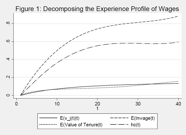
62

63

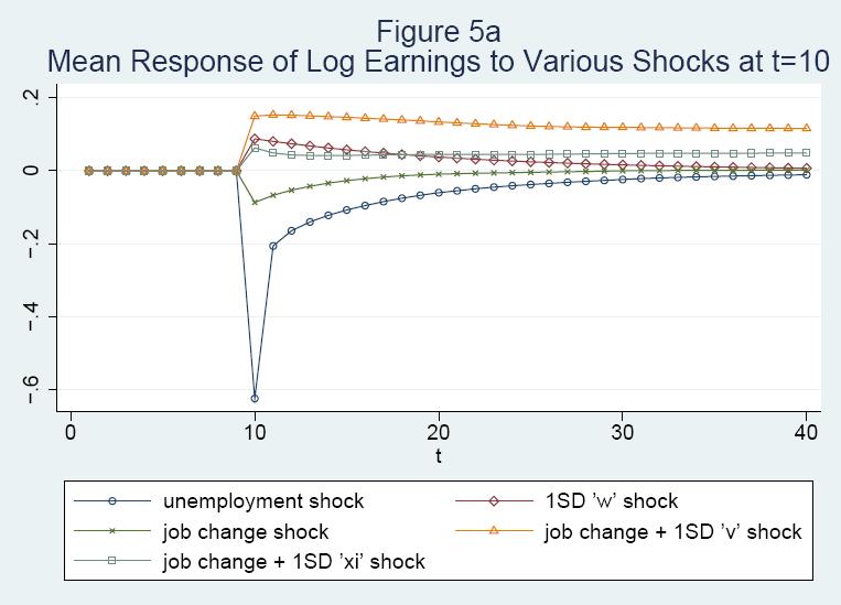
64

65

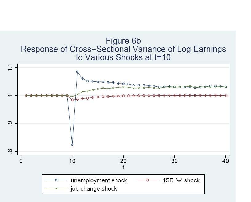
66

67

68 Table A1 Composition of PSID Sample before Sample Selection Based on Employment Status. Emp. Status Percentage Working Temp. Laidoff 1.48 Unemployed 5.9 Retired 0.87 Disabled 1.85 Housewife 0.19 Student 1.17 Other 0.56 The table presents the composition of the PSID sample, in terms of employment status, before we impose any sample restrictions based on employment status. The sample here meets all selection criteria which are not based on employment status. Table A2 Percentage of Observations Excluded Based on Employment Status. PE Percentage PE Percentage PE Percentage PE Percentage (a) (b) The table presents the percentage of observations excluded, based on employment status at the survey date, for each value of potential experience (PE). (a) All students at PE=1. (b) Of these, 13.5 are retired, 7.5 disabled. Table A3 Distribution of Number of Observations Contributed Per Individual in PSID Sample. Percentile Min 5% 25% 50% 75% 95% Max Number of observations per individual The table presents the cross-sectional distribution, across individuals, of the number of observations contributed to the sample by individual. Lead values are excluded.

69

70

71

72

73