Short-Term. Scheduling

Transcription

1 Short-Term 15 Scheduling PowerPoint presentation to accompany Heizer, Render, Munson Operations Management, Twelfth Edition Principles of Operations Management, Tenth Edition PowerPoint slides by Jeff Heyl 15-1

2 Short-Term Scheduling The objective of scheduling is to allocate and prioritize demand (generated by either forecasts or customer orders) to available facilities 15-2

3 Importance of Short-Term Scheduling Effective and efficient scheduling can be a competitive advantage Faster movement of goods through a facility means better use of assets and lower costs Additional capacity resulting from faster throughput improves customer service through faster delivery Good schedules result in more dependable deliveries 15-3

4 Scheduling Decisions TABLE 15.1 Scheduling Decisions ORGANIZATION Alaska Airlines Arnold Palmer Hospital University of Alabama Amway Center Lockheed Martin Factory MANAGERS SCHEDULE THE FOLLOWING Maintenance of aircraft Departure timetables Flight crews, catering, gate, ticketing personnel Operating room use Patient admissions Nursing, security, maintenance staffs Outpatient treatments Classrooms and audiovisual equipment Student and instructor schedules Graduate and undergraduate courses Ushers, ticket takers, food servers, security personnel Delivery of fresh foods and meal preparation Orlando Magic games, concerts, arena football Production of goods Purchases of materials Workers 15-4

5 Scheduling Issues Scheduling deals with the timing of operations The task is the allocation and prioritization of demand Significant factors are 1) Forward or backward scheduling 2) Finite or infinite loading 3) The criteria for sequencing jobs 15-5

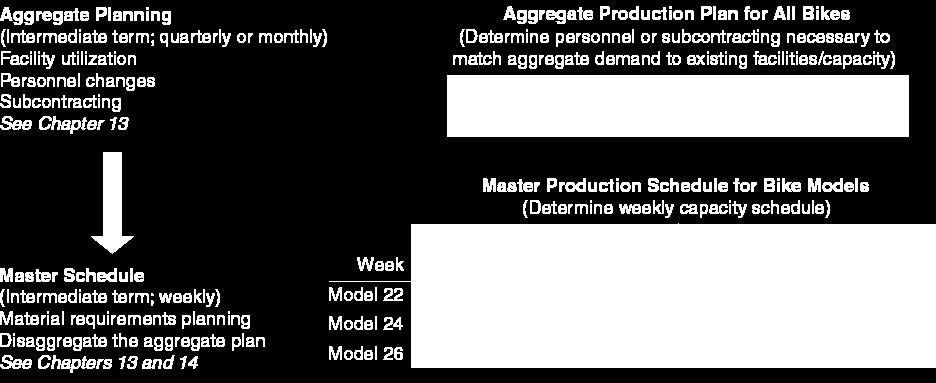
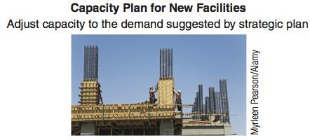
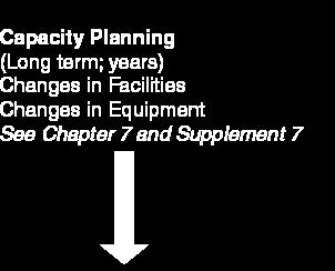
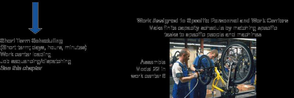
6 Scheduling Flow Figure

7 Forward and Backward Scheduling Forward scheduling starts as soon as the requirements are known Produces a feasible schedule though it may not meet due dates Frequently results in buildup of work-inprocess inventory Now Due Date 15-7

8 Forward and Backward Scheduling Backward scheduling begins with the due date and schedules the final operation first Schedule is produced by working backwards though the processes Resources may not be available to accomplish the schedule Now Due Date 15-8

9 Forward and Backward Backward scheduling begins with the due date and schedules the final operation first Schedule is produced by working backwards though the processes Resources may not be available to accomplish the schedule Scheduling Now Due Date 15-9

10 Finite and Infinite Loading Assigning jobs to work stations Finite loading assigns work up to the capacity of the work station All work gets done Due dates may be pushed out Infinite loading does not consider capacity All due dates are met Capacities may have to be adjusted 15-10

11 Scheduling Criteria 1. Minimize completion time 2. Maximize utilization of facilities 3. Minimize work-in-process (WIP) inventory 4. Minimize customer waiting time 15-11

12 TABLE 15.2 Different Processes/ Different Approaches Different Processes Suggest Different Approaches to Scheduling Process-focused facilities (job shops) Scheduling to customer orders where changes in both volume and variety of jobs/clients/patients are frequent Schedules are often due-date focused, with loading refined by finite loading techniques Examples: foundries, machine shops, cabinet shops, print shops, many restaurants, and the fashion industry Repetitive facilities (assembly lines) Schedule module production and product assembly based on frequent forecasts Finite loading with a focus on generating a forward-looking schedule JIT techniques are used to schedule components that feed the assembly line Examples: assembly lines for washing machines at Whirlpool and automobiles at Ford 15-12

13 TABLE 15.2 Different Processes/ Different Approaches Different Processes Suggest Different Approaches to Scheduling Product-focused facilities (continuous) Schedule high-volume finished products of limited variety to meet a reasonably stable demand within existing fixed capacity Finite loading with a focus on generating a forward-looking schedule that can meet known setup and run times for the limited range of products Examples: huge paper machines at International Paper, beer in a brewery at Anheuser-Busch, and potato chips at Frito-Lay 15-13

14 Scheduling Process- Focused Facilities High-variety, low volume Production items differ considerably Schedule incoming orders without violating capacity constraints Scheduling can be complex 15-14

15 Loading Jobs Assign jobs so that costs, idle time, or completion time are minimized Two forms of loading Capacity oriented Assigning specific jobs to work centers 15-15

16 Input-Output Control Identifies overloading and underloading conditions Prompts managerial action to resolve scheduling problems Can be maintained using ConWIP cards that control the scheduling of batches 15-16

17 Input-Output Control Example Figure 15.2 Work Center DNC Milling (in standard hours) Week Ending 6/6 6/13 6/20 6/27 7/4 7/11 Planned Input Actual Input Cumulative Deviation Planned Output Actual Output Cumulative Deviation Cumulative Change in Backlog

18 Input-Output Control Example Figure 15.2 Welding Work Center (in standard hours) Week Ending 6/6 6/13 6/20 6/27 7/4 7/11 Planned Input Actual Input Explanation: Cumulative Deviation 270 input, output implies 0 change Planned Output Explanation: 250 input, Actual Output output implies Cumulative Deviation change Cumulative Change in Backlog

19 Input-Output Control Example Options available to operations personnel include: Correcting performances Increasing capacity Increasing or reducing input to the work center 15-19

20 Gantt Charts Load chart shows the loading and idle times of departments, machines, or facilities Displays relative workloads over time Schedule chart monitors jobs in process All Gantt charts need to be updated frequently to account for changes 15-20

21 Gantt Load Chart Example Figure 15.3 Work Center Day Monday Tuesday Wednesday Thursday Friday Metalworks Job 349 Job 350 Mechanical Job 349 Job 408 Electronics Job 408 Job 349 Painting Job 295 Job 408 Job 349 Processing Unscheduled Center not available 15-21

22 Gantt Schedule Chart Example Figure 15.4 Job Day 1 Day 2 Day 3 Day 4 Day 5 Day 6 Day 7 Day 8 Start of an activity End of an activity A Scheduled activity time allowed B Maintenance Actual work progress C Now Nonproduction time Point in time when chart is reviewed 15-22

23 Assignment Method A special class of linear programming models that assigns tasks or jobs to resources Objective is usually to minimize cost or time Only one job (or worker) is assigned to one machine (or project) 15-23

24 Assignment Method Build a table of costs or time associated with particular assignments TYPESETTER JOB A B C R-34 $11 $14 $ 6 S-66 $ 8 $10 $11 T-50 $ 9 $12 $

25 Assignment Method 1. Create zero opportunity costs by repeatedly subtracting the lowest costs from each row and column 2. Draw the minimum number of vertical and horizontal lines necessary to cover all the zeros in the table. If the number of lines equals either the number of rows or the number of columns, proceed to step 4. Otherwise proceed to step

26 Assignment Method 3. Subtract the smallest number not covered by a line from all other uncovered numbers. Add the same number to any number at the intersection of two lines. Return to step Optimal assignments are at zero locations in the table. Select one, draw lines through the row and column involved, and continue to the next assignment

27 Assignment Example Typesetter A B C Job R-34 $11 $14 $ 6 S-66 $ 8 $10 $11 T-50 $ 9 $12 $ 7 Typesetter Step 1a - Rows A B C Job R-34 $ 5 $ 8 $ 0 S-66 $ 0 $ 2 $ 3 T-50 $ 2 $ 5 $ 0 Step 1b - Columns Typesetter A B C Job R-34 $ 5 $ 6 $ 0 S-66 $ 0 $ 0 $ 3 T-50 $ 2 $ 3 $

28 Assignment Example Typesetter Step 2 - Lines A B C Job R-34 $ 5 $ 6 $ 0 S-66 $ 0 $ 0 $ 3 T-50 $ 2 $ 3 $ 0 Smallest uncovered number Because only two lines are needed to cover all the zeros, the solution is not optimal Step 3 - Subtraction The smallest uncovered number is 2 so this is subtracted from all other uncovered numbers and added to numbers at the intersection of lines Typesetter A B C Job R-34 $ 3 $ 4 $ 0 S-66 $ 0 $ 0 $ 5 T-50 $ 0 $ 1 $

29 Assignment Example Typesetter Step 2 - Lines A B C Job R-34 $ 3 $ 4 $ 0 S-66 $ 0 $ 0 $ 5 T-50 $ 0 $ 1 $ 0 Because three lines are needed, the solution is optimal and assignments can be made Step 4 - Assignments Start by assigning R-34 to worker C as this is the only possible assignment for worker C. Job T-50 must go to worker A as worker C is already assigned. This leaves S-66 for worker B. Typesetter A B C Job R-34 $ 3 $ 4 $ 0 S-66 $ 0 $ 0 $ 5 T-50 $ 0 $ 1 $

30 Assignment Example Typesetter A B C Job R-34 $11 $14 $ 6 S-66 $ 8 $10 $11 T-50 $ 9 $12 $ 7 Typesetter A B C Job R-34 $ 3 $ 4 $ 0 S-66 $ 0 $ 0 $ 5 T-50 $ 0 $ 1 $ 0 From the original cost table Minimum cost = $6 + $10 + $9 = $

31 Sequencing Jobs Specifies the order in which jobs should be performed at work centers Priority rules are used to dispatch or sequence jobs FCFS: First come, first served SPT: Shortest processing time EDD: Earliest due date LPT: Longest processing time 15-31

32 Performance Criteria Flow time the time between the release of a job to a work center until the job is finished Average completion time = Utilization metric = Average number of jobs in the system = Average job lateness = Sum of total flow time Number of jobs Total job work (processing) time Sum of total flow time Sum of total flow time Total job work (processing) time Total late days Number of jobs 15-32

33 Performance Criteria Flow time the time between the release of a job to a work center until the job is finished Sum of total flow time Average completion time = Number of jobs Job lateness = Max{0, yesterday + flow time due date} Total job work (processing) time Utilization metric = Sum of total flow time Average number of jobs in the system = Average job lateness = Sum of total flow time Total job work (processing) time Total late days Number of jobs 15-33

34 Sequencing Example Apply the four popular sequencing rules to these five jobs Job Job Work (Processing) Time (Days) Job Due Date (Days) A 6 8 B 2 6 C 8 18 D 3 15 E

35 Sequencing Example FCFS: Sequence A-B-C-D-E Job Sequence Job Work (Processing) Time Flow Time Job Due Date Job Lateness A B C D E

36 Sequencing Example FCFS: Sequence A-B-C-D-E Average completion time = Sum of total flow time Number of jobs = 77/5 = 15.4 days Total job work (processing) time Utilization metric = Sum of total flow time = 28/77 = 36.4% Average number of jobs in the system = Sum of total flow time Total job work time = 77/28 = 2.75 jobs Average job lateness = Total late days Number of jobs = 11/5 = 2.2 days 15-36

37 Sequencing Example SPT: Sequence B-D-A-C-E Job Sequence Job Work (Processing) Time Flow Time Job Due Date Job Lateness B D A C E

38 Sequencing Example SPT: Sequence B-D-A-C-E Average completion time = Sum of total flow time Number of jobs = 65/5 = 13 days Total job work time Utilization metric = Sum of total flow time = 28/65 = 43.1% Average number of jobs in the system Sum of total flow time = = 65/28 = 2.32 jobs Total job work time Average job lateness = Total late days Number of jobs = 9/5 = 1.8 days 15-38

39 Sequencing Example EDD: Sequence B-A-D-C-E Job Sequence Job Work (Processing) Time Flow Time Job Due Date Job Lateness B A D C E

40 Sequencing Example EDD: Sequence B-A-D-C-E Average completion time = Sum of total flow time Number of jobs = 68/5 = 13.6 days Total job work time Utilization metric = Sum of total flow time = 28/68 = 41.2% Average number of jobs in the system Sum of total flow time = = 68/28 = 2.43 jobs Total job work time Average job lateness = Total late days Number of jobs = 6/5 = 1.2 days 15-40

41 Sequencing Example LPT: Sequence E-C-A-D-B Job Sequence Job Work (Processing) Time Flow Time Job Due Date Job Lateness E C A D B

42 Sequencing Example LPT: Sequence E-C-A-D-B Average completion time = Sum of total flow time Number of jobs = 103/5 = 20.6 days Total job work time Utilization metric = Sum of total flow time = 28/103 = 27.2% Average number of jobs in the system Sum of total flow time = = 103/28 = 3.68 jobs Total job work time Average job lateness = Total late days Number of jobs = 48/5 = 9.6 days 15-42

43 Sequencing Example Summary of Rules Rule Average Completion Time (Days) Utilization Metric (%) Average Number of Jobs in System Average Lateness (Days) FCFS SPT EDD LPT

44 Comparison of Sequencing Rules No one sequencing rule excels on all criteria 1. SPT does well on minimizing flow time and number of jobs in the system But SPT moves long jobs to the end which may result in dissatisfied customers 2. FCFS does not do especially well (or poorly) on any criteria but is perceived as fair by customers 3. EDD minimizes maximum lateness 15-44

45 Critical Ratio (CR) An index number found by dividing the time remaining until the due date by the work time remaining on the job Jobs with low critical ratios are scheduled ahead of jobs with higher critical ratios Performs well on average job lateness criteria Time remaining CR = = Workdays remaining Due date Today's date Work (lead) time remaining 15-45

46 Critical Ratio Example Currently Day 25 JOB DUE DATE WORKDAYS REMAINING A 30 4 B 28 5 C 27 2 JOB CRITICAL RATIO PRIORITY ORDER A (30-25)/4 = B (28-25)/5 =.60 1 C (27-25)/2 = With CR < 1, Job B is late. Job C is just on schedule and Job A has some slack time

47 Critical Ratio Technique 1. Determine the status of a specific job 2. Establish relative priorities among jobs on a common basis 3. Adjust priorities automatically for changes in both demand and job progress 4. Dynamically track job progress 15-47

48 Sequencing N Jobs on Two Machines: Johnson's Rule Works with two or more jobs that pass through the same two machines or work centers Minimizes total production time and idle time An N/2 problem, N number of jobs through 2 workstations 15-48

49 Johnson s Rule 1. List all jobs and times for each work center 2. Select the job with the shortest activity time. If that time is in the first work center, schedule the job first. If it is in the second work center, schedule the job last. Break ties arbitrarily. 3. Once a job is scheduled, it is eliminated from the list 4. Repeat steps 2 and 3 working toward the center of the sequence 15-49

50 Johnson s Rule Example JOB WORK CENTER 1 (DRILL PRESS) WORK CENTER 2 (LATHE) A 5 2 B 3 6 C 8 4 D 10 7 E

51 Johnson s Rule Example JOB WORK CENTER 1 (DRILL PRESS) WORK CENTER 2 (LATHE) A 5 2 B 3 6 C 8 4 B E D C A D 10 7 E

52 Johnson s Rule Example JOB WORK CENTER 1 (DRILL PRESS) WORK CENTER 2 (LATHE) A 5 2 B 3 6 C 8 4 B E D C A D 10 7 E 7 12 Time WC 1 B E D C A Idle WC 2 Job completed 15-52

53 Johnson s Rule Example JOB WORK CENTER 1 (DRILL PRESS) WORK CENTER 2 (LATHE) A 5 2 B 3 6 C 8 4 B E D C A D 10 7 E 7 12 Time WC 1 B E D C A Idle WC 2 B E D C A Time Job completed B E D C A 15-53

54 Limitations of Rule-Based Dispatching Systems 1. Scheduling is dynamic and rules need to be revised to adjust to changes 2. Rules do not look upstream or downstream 3. Rules do not look beyond due dates 15-54

55 Finite Capacity Scheduling Overcomes disadvantages of rule-based systems by providing an interactive, computer-based graphical system May include rules and expert systems or simulation to allow real-time response to system changes FCS allows the balancing of delivery needs and efficiency 15-55

56 Finite Capacity Scheduling Planning Data Master schedule BOM Inventory Priority rules Expert systems Simulation models Interactive Finite Capacity Scheduling Routing files Work center information Tooling and other resources Setups and run time Figure

57 Finite Capacity Scheduling Figure

58 Scheduling Services Service systems differ from manufacturing MANUFACTURING Schedules machines and materials Inventories used to smooth demand Machine-intensive and demand may be smooth Scheduling may be bound by union contracts Few social or behavioral issues Schedule staff SERVICES Seldom maintain inventories Labor-intensive and demand may be variable Legal issues may constrain flexible scheduling Social and behavioral issues may be quite important 15-58

59 Scheduling Services Hospitals have complex scheduling systems to handle complex processes and material requirements Banks use a cross-trained and flexible workforce and part-time workers Retail stores use scheduling optimization systems that track sales, transactions, and customer traffic to create work schedules in less time and with improved customer satisfaction 15-59

60 Scheduling Services Airlines must meet complex FAA and union regulations and often use linear programming to develop optimal schedules 24/7 operations like police/fire departments, emergency hot lines, and mail order businesses use flexible workers and variable schedules, often created using computerized systems 15-60

61 Scheduling Service Employees With Cyclical Scheduling Objective is to meet staffing requirements with the minimum number of workers Schedules need to be smooth and keep personnel happy Many techniques exist from simple algorithms to complex linear programming solutions 15-61

62 Cyclical Scheduling Example 1. Determine the staffing requirements 2. Identify two consecutive days with the lowest total requirements and assign these as days off 3. Make a new set of requirements subtracting the days worked by the first employee 4. Apply step 2 to the new row 5. Repeat steps 3 and 4 until all requirements have been met 15-62

63 Cyclical Scheduling Example DAY M T W T F S S Staff required M T W T F S S Employee Capacity (Employees) Excess Capacity 15-63

64 Cyclical Scheduling Example DAY M T W T F S S Staff required M T W T F S S Employee Employee Capacity (Employees) Excess Capacity 15-64

65 Cyclical Scheduling Example DAY M T W T F S S Staff required M T W T F S S Employee Employee Employee Capacity (Employees) Excess Capacity 15-65

66 Cyclical Scheduling Example DAY M T W T F S S Staff required M T W T F S S Employee Employee Employee Employee Capacity (Employees) Excess Capacity 15-66

67 Cyclical Scheduling Example DAY M T W T F S S Staff required M T W T F S S Employee Employee Employee Employee Employee Capacity (Employees) Excess Capacity 15-67

68 Cyclical Scheduling Example DAY M T W T F S S Staff required M T W T F S S Employee Employee Employee Employee Employee Employee Capacity (Employees) Excess Capacity 15-68

69 Cyclical Scheduling Example DAY M T W T F S S Staff required M T W T F S S Employee Employee Employee Employee Employee Employee Employee 7 1 Capacity (Employees) Excess Capacity

70 All rights reserved. No part of this publication may be reproduced, stored in a retrieval system, or transmitted, in any form or by any means, electronic, mechanical, photocopying, recording, or otherwise, without the prior written permission of the publisher. Printed in the United States of America