Canadian Labour Market and Skills Researcher Network

Transcription

1 Canadian Labour Market and Skills Researcher Network Working Paper No. 89 Human Capital Prices, Productivity and Growth Audra J. Bowlus University of Western Ontario Chris Robinson University of Western Ontario December 2011 CLSRN is funded by the Social Sciences and Humanities Research Council of Canada (SSHRC) under its Strategic Knowledge Clusters Program. Research activities of CLSRN are carried out with support of Human Resources and Skills Development Canada (HRSDC). All opinions are those of the authors and do not reflect the views of HRSDC or the SSHRC.

2 Human Capital Prices, Productivity and Growth Audra J. Bowlus University of Western Ontario Chris Robinson University of Western Ontario August 2011 Abstract Separate identification of the price and quantity of human capital has important implications for understanding key issues in economics. Price and quantity series are derived for four education levels. The price series are highly correlated and they exhibit a strong secular trend. Three resulting implications are explored: the rising college premium is found to be driven more by relative quantity than relative price changes, life-cycle wage profiles are readily interpretable as reflecting optimal human capital investment paths using the estimated price series, and adjusting the labor input for quality increases dramatically reduces the contribution of MFP to growth. Keywords: Human Capital, Productivity and Growth. JEL Codes: J24, J31, O47 The authors wish to thank Lance Lochner and Todd Stinebrickner for helpful comments and discussion. We thank the editor and referees for detailed comments on earlier drafts. We also thank participants in seminars at the University of Virginia, the University of Guelph, McMaster University, the University of British Columbia, Wlifrid Laurier University and conference sessions at the 2006 CEA Annual Meetings, the first annual UM/MSU/UWO Labor Economics Day, the CIBC Human Capital, Productivity and the Labour Market Conference, and the 2011 CLSRN Annual Conference. This work was supported by the CIBC Human Capital and Productivity Centre and the Canadian Social Sciences and Humanities Research Council. Department of Economics, University of Western Ontario, London, ON N6A 5C2, Canada, abowlus@uwo.ca. Department of Economics, University of Western Ontario, London, ON N6A 5C2, Canada, robinson@uwo.ca. 1

3 1 Introduction The flow from human capital is by far the most important input in the world economy. The estimated share of labor in the U.S. and most of the OECD countries, for example, is about two thirds. There is quite general agreement that human capital plays a significant role in the determination of living standards. Human capital theory has been the basis of a huge literature studying the determination of earnings and inequality. 1 The recent rise in the skill premium and inequality in the U.S. has stimulated a large literature, based on the human capital framework, to provide an explanation. 2 At the same time, it has exposed a continuing weakness of human capital theory due to an inherent under-identification problem. This is a problem for many standard microeconomic based analysis of earnings patterns, but it is also a problem for macroeconomic growth studies. Payments to human capital may be directly observed, but a payment is a product of a price and a quantity. In general, neither the quantity nor the price of human capital is directly observable. Thus, when payment (wage) differences are observed between any observable groups, say by education level or by country, in general it is not possible to distinguish whether the difference is due to a difference in prices or a difference in quantities, or some combination of the two. This has important implications for our understanding of many key issues in labor economics and macroeconomics, including the rising college premium, rising inequality, sources of growth and life-cycle productivity profiles. With a small number of exceptions, the vast literature on human capital has ignored this identification problem. 3 In most cases implicit identification assumptions are made, usually representing one of two extremes: either constant quantities or constant prices over time. Assessing the contribution of human capital to output, living standards and growth is hampered by serious conceptual and measurement problems due to this identification issue. It is well recognized that the quantity of the labor input cannot simply be measured by total hours. 4 The implicit identification strategy typically adopted to 1 Seminal works include Becker (1964), Ben-Porath (1967), and Mincer (1974). 2 See, for example, Katz and Murphy (1992), Card and Lemieux (2001), and the survey by Katz and Autor (1999), for traditional labor economics approaches, and Krusell et al.(2000), Guvenen and Kuruscu (2007) and Huggett, Ventura and Yaron (2006) in the macroeconomics literature 3 The relatively few exceptions include Heckman, Lochner and Taber (1998), Weiss and Lillard (1978), and Huggett, Ventura and Yaron (2006). 4 The importance of this problem was recently emphasized by Solow (2001, p.174): alternative ways of measuring human capital can make a big-time difference in the plausible interpretation of economic growth, so it is really important to come to some scientific agreement on the best way to deal with human capital as in input (and as an output, don t forget) and then to implement it. 1

4 construct an alternative to hours for a given country is that quantities within an observable type of labor are constant and that all wage changes are due to changes in prices. The college premium literature provides a similar example where relative payments are typically taken as relative prices which implicitly assumes that relative quantities are constant. The early literature on human capital in a life-cycle context studied the implications of optimal investment in human capital for log wage profiles by age or experience. Following influential papers by Ben-Porath (1967), Heckman (1976), Rosen (1976) and others, human capital theory became the dominant framework for analyzing life-cycle earnings. This framework has spread from its base in labor economics and is increasingly used in the modern macroeconomics literature. Recent examples include Huggett, Ventura and Yaron (2006) and Guvenen and Kuruscu (2007). 5 Empirical examination of experience profiles, based on the human capital framework, has a long tradition going back to Mincer (1974). The Mincer inspired literature was re-examined by Murphy and Welch (1990), and more recently by Heckman, Lochner and Todd (2002). The large number of papers indicates the continuing importance of this topic for economists in understanding wage patterns. A common feature of the life-cycle human capital literature provides a contrasting example to the standard identification approach, representing the other extreme, where the life-cycle profile of payments is assumed to be the same as the life-cycle profile of the (supplied) quantity of human capital which implicitly assumes that the price is constant over the life-cycle. In this paper we address the identification problem directly and construct price series for four possible types of human capital associated with commonly used education groups: high school dropouts, high school graduates, some college and college graduates. There is no simple solution to the problem. Some assumptions have to be made. Our assumptions are discussed in detail so that they may be contrasted with the implicit, and often in our view, extreme assumptions generally made in the literature. The price series that are constructed for these four education groups turn out to be surprisingly highly correlated over the period 1963 to 2008 despite their large differences in skill level. The series also exhibit patterns that deviate substantially from wages, implying that wages are not good proxies for prices and that quantities of human capital associated with a given observable education type change over time. Both of these results have major implications for understanding the evolution of wages, wage premia and the human capital input in the aggregate production function 5 A separate but related development in the literature has been the estimation or calibration of general equilibrium models of human capital accumulation over the life cycle. Examples include Heckman, Lochner and Taber (1998), Imai and Keane (2004), Lee (2005) and Hansen and Imrohoroglu (2007). 2

5 (and hence, total factor productivity). In Section 2 the basic identification issue is discussed. This is not a problem unique to human capital. The possible change in quantities of human capital associated with a given observable education type over time or across countries is identical to the problem of an unobserved change in quality over time in a product. A prominent example that has received much attention in the macroeconomic literature is the identification of an appropriate price series for various forms of physical capital inputs, particularly the input from computers. It is clear that conventional methods of constructing a measure of inputs over time in the case of computers fails very badly. Measures based on physical numbers, price or total value all drastically underestimate the computer input. The identification issue for capital inputs has received a lot of attention. Unfortunately, due to observability issues, the solution for human capital is more difficult than for many types of physical capital. Section 3 details our identification approach and estimation methodology. Our main identification approach is a variation on the flat spot method first proposed in Heckman, Lochner and Taber (1998). A methodology is developed for choosing a flat spot for each education group, i.e. an age range towards the end of the life-cycle when supplied human capital is constant, that differs from Heckman, Lochner and Taber (1998). We use data from the U.S. March Current Population Surveys (MCPS) covering earnings years 1963 to Section 4 describes the MCPS and the implementation of the estimation methodology on these data. Section 5 presents the estimated price series for the four human capital types. The price series all show substantial movement over the 1963 to 2008 period and the patterns are robust to a number of validity checks and sensitivity analysis. Perhaps the most surprising result is a very high correlation between the series from the lowest education group (high school dropouts) to the highest (college graduates). All of the series exhibit an increase in the price from 1963 to the mid-1970s followed by a substantial decline through the 1980s and 1990s that is interrupted by plateaus or recoveries coming out of the recessions of the early 1980s and the early 1990s. Finally, all four prices are relatively flat after The price series of Section 5 have many important implications for both microeconomic and macroeconomic issues. First, since the series are highly correlated, the movement in relative prices is quite modest implying that a substantial part of the variation in the college premium is due to variation in the relative quantities of human capital associated with each observed education group. Second, since the price varies over the life-cycle, the path of a cohort s wages or earnings does 3

6 not identify the path of (supplied) human capital. Third, the high correlation also implies that a homogeneous model may be a good approximation for macroeconomic models dealing with secular trends. This has the great advantage of a simplified and easily interpretable labor input which may be constructed by dividing total payments to labor by the estimated price series. The use of this measure of the labor input suggests a very different path for total factor productivity (TFP) than is derived from conventional aggregate labor input measures. Each of these implications is explored in turn. Section 6 re-examines the college premium, and decomposes the change in relative wages into the separate components of relative price and quantity changes. It shows that relative quantity changes are at least as important as relative price changes in explaining the path of the average college premium. In addition, selection effects on relative quantities implied by cohort education patterns can also explain the age patterns documented in Card and Lemieux (2001). Section 7 shows that the life-cycle pattern of quantities of human capital for each cohort implied by the price series is consistent with human capital theory and, in contrast to the usual constant price assumption, yields readily interpretable cross cohort patterns. The maintained hypothesis explored in this paper is that college graduates have the same type of college graduate human capital over time. In Section 8 we contrast this hypothesis with an alternative skill biased technological change hypothesis under which there was a change in vintage type, coinciding with the widespread introduction of micro computers, that resulted in an increase in the college premium for the young ( new vintage ) college graduates, but not for the ( old vintage ) older college graduates, as described in Card and Lemieux (2001). The primary difference between the two hypotheses is their different implications for the time path of vintage effects. Under the hypothesis explored in this paper vintage effects occur through selection effects and technological improvement in human capital production which occur continuously. The alternative hypothesis is that vintage effects come about through changes in vintage types rather than through quantity changes due to selection effects and technological improvement. Thus, for the maintained hypothesis of this paper, the time path of the vintage effects is constrained by the selection effects implied by cohort education patterns combined with technological improvement in the production of human capital. For the alternative hypothesis the pattern is constrained by the timing of the vintage type change. The different constraints result in different predictions for the pattern of vintage effects. Our test results show that the evidence is consistent with our maintained hypothesis. 4

7 Section 9 uses the estimates of the price series from Section 5 to construct measures of the total labor input and a new TFP series for the U.S. over the period The results show that conventional quality adjustment to the labor input results in substantial underestimation in the growth of the true labor input, and hence a large overestimate of increases in TFP. Section 10 provides some final discussion and summary. 2 The Price and Quantity of Human Capital: Identification In standard human capital models with competitive firms the hourly wage is the product of a price and a quantity w it = λ t E it, (1) where E it is the amount of human capital supplied to the firm (number of efficiency units) by worker i in time period t, and λ t is the rental price paid for renting a single unit of human capital (the price of an efficiency unit). In a homogeneous human capital model there is a single price, λ t, and wages differ across workers in any given time period because of differences in the amount of (homogeneous) human capital they supply. Over time a worker s wage could change either because of a change in the quantity of efficiency units supplied, or because of a change in the price. However, all relative wage changes are due to relative changes in the quantity of efficiency units supplied by each type. This is the main consequence of the efficiency units approach in a homogeneous human capital model. In heterogeneous human capital models, an efficiency units approach is retained within some exogenously defined worker type (e.g. college graduate) but is abandoned across types. With two worker types (e.g. college and non-college) there are two factors and two prices with wages given as follows (suppressing the individual and time subscript for convenience): w a = λ a E a and w b = λ b E b where λ a and λ b are the prices of efficiency units of type a and b, respectively, and E a and E b are the number of efficiency units of type a and b supplied by type a and b workers, respectively. Within type, the wage implications are the same as the homogeneous human capital model. For relative wages across types the implications are potentially different. Since there are now two prices, changes in relative wages between the two types reflect changes in relative quantities, E a /E b, and changes in relative prices, λ a /λ b. Identification of the prices and quantities of human capital is a difficult problem in both homogeneous and heterogeneous human capital models. The hourly wage is observed, but its two 5

8 components are not. This is the fundamental under-identification property of human capital models. 6 In heterogeneous human capital models used in the skill-biased technological change literature, the problem is implicitly solved by assuming that the quantities of human capital associated with any observed education level (or education/age group) are the same over time. This permits the identification of changes in the skill price ratio from changes in the wage ratio. However, this is a very strong assumption. It assumes no selection effects on average quantities by education group even tough there been large increases in the fraction of successive birth cohorts choosing higher levels of education. It also rules out technological improvement in human capital production functions. 7 Figure 1 plots completed schooling level for male birth cohorts from 1931 to It shows that over these cohorts there have been very large changes. 8 For example, the fraction of the birth cohort going to college increased by 50 % between the 1937 and 1946 birth cohorts (from below 20% to over 30 %.) Since there is a strong correlation between measures of ability and the highest level of completed schooling, these large secular changes in completed schooling levels may be expected to have significant selection effects on the average ability, and hence human capital, associated with each observed schooling level. 9 Further, since major quality improvements due to technological change have been found for capital inputs such as computers, it is surprising that they have been generally ruled out for the labor input. We argue that technological improvement in human capital production functions can produce workers of a given observed type, such as education level, that can do more, in the same sense as more recent computers can do more, especially at the upper level as knowledge advances. More recent vintages of physics PhDs, for example, are likely to have received more value added (more advanced knowledge) through the education process, than earlier PhDs. The identification problem and technological change in human capital production functions was 6 For a simple static problem within a market with a single price, the identification problem is solved trivially by a normalization of one of the components. However, more generally, for static problems such as identifying the source of wage differences across countries with (potentially) different prices, or dynamic problems such as changes over time in the skill price ratio, human capital models have this under-identification property. For dynamic problems, the under-identification problem follows from the standard under-identification of age, year and cohort effects. 7 If technological change in human capital production is not taken into account, the labor input in aggregate production functions will be underestimated which results in an apparent technological improvement or TFP increase in the product market production functions. Similar mis-attribution can happen with capital mis-measurement. Greenwood, Hercowitz and Krusell (1997) investigate this issue and provide estimates to suggest that the magnitude in the capital input case is important. Estimates in Section 9 below suggest that the magnitude in the labor input case is also very important. 8 The data source for Figure 1 is the MCPS. This is described in more detail in Section 4 below. 9 There is a large amount of evidence suggesting a high correlation between observed ability measures and educational attainment. For example, the correlation between highest degree completed and scores from the Armed Forces Qualification Test for individuals in the 1979 National Longitudinal Survey of Youth is

9 discussed in a related context in Weiss and Lillard (1978) who tried to distinguish between time and vintage effects in the earnings of scientists. They documented the fact that there was a difference in the life-cycle path of earnings for the more recent vintages of scientists in the period they studied. Since they were unable to employ a separately identified price series of the type derived in this paper, Weiss and Lillard (1978) were cautious about their interpretation of the vintage effects that they found. Nevertheless, they did conclude that there were substantial vintage effects over the period that they studied. This suggests that the assumption of no change in quantities within observable types may well be a bad one. The primary maintained hypothesis in this paper is that there are a number of types of human capital, as indicated by education group, that are the same over time, allowing for a meaningful definition of changes in quantities within type over time. This is the standard efficiency units assumption within types that is common in the literature. In this framework, the time effects of Weiss and Lillard (1978) can be interpreted as price effects, while the vintage effects can be interpreted as quantity differences across cohorts due to selection effects and technological improvements in human capital production functions. This is a parsimonious specification of vintage effects since it maintains a constant number of human capital types and prices. The main objective of the paper is to identify prices and quantities within this framework. However, one interpretation of changes in relative wages by skill is that vintage effects may take the form of introducing new types of human capital (and hence new prices) that are not directly comparable to the old types. This complicates an already difficult identification problem by introducing more types. In general it is difficult to distinguish quantity changes within the same type from changes in types using wage data. In Section 8 below we explore this further in the context of a possible vintage type change with the introduction of computers. 3 Estimation Methodology The main identification approach used in this paper is the flat spot method which can be used with either homogeneous or heterogeneous models. Both models assume an efficiency units structure at some disaggregated level. Under the assumption of competitive markets for each human capital type, following equation (1), log wages in these models for any individual i of a particular type are 7

10 given by 10 lnw it = lnλ t + lne it. (2) Given two periods in which the log (supplied) efficiency units of individual i are equal across periods (the individual s flat spot ) the change in log prices across periods is given by the change in the individual s log wages across periods. That is: lnλ t+1 lnλ t = [lnw it+1 lnw it ] [lne it+1 lne it ] = [lnw it+1 lnw it ]. (3) This implies that, given two samples for which the sample mean log (supplied) efficiency units are equal across periods, the change in log wages across periods can be estimated by the change in the mean log wages in the sample across periods. That is: Mean[lnE it ] = Mean[lnE it+1 ] Mean[lnw it+1 ] Mean[lnw it ] = lnλ t+1 lnλ t. (4) The flat spot method was first proposed in Heckman, Lochner and Taber (1998). Flat spot methods estimate the price change by restricting estimation of equation (4) to samples consisting only of individuals in their flat spot range, to satisfy the requirement that Mean[lnE it ] = Mean[lnE it+1 ]. For each education group (human capital type) there is assumed to be an age range towards the end of the working life where (supplied) efficiency units are constant, a typical feature of Ben-Porath based models of optimal human capital investment over the life-cycle Choosing the Flat Spot Regions The most important problem to be solved in implementing the flat spot method is the choice of the flat spot regions in supplied efficiency units for the four education groups. Mincer and Ben-Porath make the important distinction between earnings capacity and observed earnings. Let the efficiency units flow per hour from the stock of human capital of individual i in period t be E it. Earnings capacity per hour is given by λ t Eit, and reflects the individual s total efficiency units, which are greater than supplied efficiency units per hour whenever investment is positive. Supplied efficiency units per hour are given by E it s it where s it is the fraction of the hour (or efficiency units within the hour) supplied to the employer for productive work rather than invested in human capital. 10 Here we have suppressed the superscript notation delineating type. 11 See Heckman, Lochner and Taber (1998), Huggett, Ventura and Yaron (2006) and Kuruscu (2006) for recent discussion of this feature of optimal life-cycle investment models. 8

11 Observed earnings per hour are thus given by λ t E it s it. The appropriate flat spot range is the flat spot in E it = E it s it, not the flat spot in the human capital stock, or E it. There is a large literature that uses the Ben-Porath model of optimal life-cycle production of human capital to interpret observed age-earnings profiles in terms of the underlying life-cycle profile of (supplied) efficiency units of human capital. Mincer s (1974) pioneering analysis documented several important features of age-earnings profiles. The profile is concave with the largest increase in the early years, rising to a peak and then declining. Mincer (1974), citing evidence from the Bureau of Labor Statistics, argued that the working life was roughly equal across education groups and that the life-cycle log earnings (or wage) profiles for all groups could be approximated using a linear term for years of schooling and a quadratic specification for years worked or experience. This resulted in a concave shape with earnings-experience profiles that were parallel across education groups, and became the standard specification. 12 This specification was extensively re-examined in Murphy and Welch (1990) using MCPS data for Murphy and Welch (1990) confirm that Mincer s emphasis on experience rather than age seems on target and show close to parallel profiles for experience defined as starting at 19, 20, 21 and 24 for dropouts, high school graduates, some college and college graduates, respectively. 13 However, they do find fault with the quadratic specification which they show results in systematic bias in the growth rate of earnings at various points in the life-cycle. Their preferred specification is a quartic. This closely approximates the unrestricted schooling-experience-cell estimates, and shows the peak of the earnings profiles at approximately 30 years of experience for all schooling groups. 14 The standard Ben-Porath model assumes a constant price so that interpretation of age-earnings profiles in this framework has associated the life-cycle profile of earnings with the life-cycle profile of (supplied) human capital. The concave shape reflects primarily the declining investment; the decline beyond the peak occurs as depreciation comes to dominate gross investment. Thus, the flat spot in this case is simply the (common) experience point where the age-earnings profiles peak. However, without the constant price assumption, the age-earnings profile reflects the product of λ t and E it at each age, as in equation (1). The flat spot in E it is not identified. Given the concave shape, choosing a flat spot interval that is too early results in price change estimates that are upward biased. That is, they include some positive change in supplied efficiency units, as net investment is 12 See, for example, Murphy and Welch (1990), and Heckman, Lochner and Todd (2006) 13 Murphy and Welch (1990), p.206, and footnote Murphy and Welch (1990), Figure 10. The only exception is dropouts, which appear to peak a little later. 9

12 still positive. Conversely, choosing an interval that is too late overestimates the price change because of the depreciation. Our identification procedure for the flat spot is to use a combination of theoretical restrictions and empirical evidence based on standard human capital theory. In the standard Ben-Porath model with neutrality, the optimal life-cycle production of human capital is determined by choosing a level of production in each period where the time invariant, upward sloped marginal cost of production equals the marginal benefit that declines over time as the remaining working life gets shorter. This yields declining human capital investment over the life cycle. The flat spot, and its variation across schooling groups, thus depends on the determinants of the marginal costs and marginal benefits and how they vary across schooling groups. The marginal benefit depends primarily on hours worked per period and the length of the working life. More educated individuals work longer hours. There is also substantial evidence that higher educated individuals retire at older ages. 15 This is the justification for Mincer s focus on experience rather than age. Given an approximately equal working life across schooling groups, the time path of the marginal benefit with experience is the same for each schooling group. Kuruscu (2006) uses a standard Ben-Porath framework, together with earnings data for males with a high school degree or less from the NLSY, to estimate a piecewise linear approximation to the marginal cost curve. The estimated marginal cost curve (Kuruscu (2006), Figure 8) results in large initial investments that rapidly decline, reaching zero well before the marginal benefit reaches zero. 16 The flat spot is reached when the marginal benefit falls below the marginal cost. If all schooling groups had the same marginal cost curve, and the time path of the marginal benefit with experience is the same for each schooling group the flat spot would occur at the same level of experience for all schooling groups. This is the standard approximation following Mincer. Given the strong correlation between ability and years of education, the marginal cost may, if anything, be lower for higher educated. This would result in later flat spot by experience for the more educated, though this would be countered to the extent that the later retirement date and higher labor supply were not sufficiently large to exactly 15 See, for example Mincer (1974), pp.8-9, Burtless and Moffitt (1985) and Ruhm (1990). 16 The estimated marginal cost curve in Kuruscu(2006) shows increasing marginal costs like the marginal cost curve from the diminishing returns Cobb-Douglas production function in Ben-Porath (1967). However, unlike the marginal cost in Ben-Porath s Figure 1, Kuruscu s estimated marginal cost curve is convex to the origin and does not start at the origin. Kuruscu contrasts the two technologies that lead to these different shaped marginal cost curves and argues that the evidence from age-earnings profiles is inconsistent with technologies that result in marginal cost curves with the original Ben-Porath shape. 10

13 counter the later entry into the labor market. While this is consistent with the flat spot occurring at the same level of experience for all schooling groups, it does not establish the appropriate common level of experience. 3.2 Cross-Section Age-Earnings Profiles In order to identify the appropriate level of experience we use evidence from cross section ageearnings profiles. Life-cycle earnings profiles from panel data do not identify the flat spot because of the basic price/quantity identification problem addressed in this paper, i.e. the price is unlikely to be constant so the flat spot in the quantity, E it, is not the same as the flat spot in observed earnings, λ t E it. In the cross section, the price, λ t, is constant across age groups, but in general cross section age-earnings profiles do not identify the flat spot in E it due to cohort effects. The approach taken here is to use the cross section data for the college group for a particular span of years when the bias from the cohort effects can be signed for this group, based on the direction of selection inferred from Figure 1. Denote the life-cycle growth of mean supplied log efficiency units for individuals age a, from birth cohort c between year t and t 1 as: g t (a) = Mean[lnE it (a, c)] Mean[lnE it 1 (a 1, c)] = [Mean[lnw it (a, c)] λ t ] [Mean[lnw it 1 (a 1, c)] λ t 1 ] where c = t a, and Mean[lnE t (a, c)] is mean supplied log efficiency units for individuals age a, from birth cohort c in year t. From the cross section in year t, the growth of mean supplied log efficiency units at age a is: g tˆ(a) = Mean[lnEit (a, c)] Mean[lnE it (a 1, c + 1)] = [Mean[lnw it (a, c)] λ t ] [Mean[lnw it (a 1, c + 1)] λ t ] The growth at age a in mean supplied log efficiency units in the cross section, Mean[lnE it (a, c)] Mean[lnE it (a 1, c + 1)] can be estimated from observed wages in the cross section given a normalization for λ t. However, this is a biased estimate of g t (a), where the bias is given by: bias = g tˆ(a) gt (a) = Mean[lnE it 1 (a 1, c)] Mean[lnE it (a 1, c + 1)] (5) In the cross section the observation for the mean supplied log efficiency units for age a 1 is taken from a different birth cohort than the mean for age a. 11

14 There are two cohort effects that cause a bias in estimating g t (a) from the cross section g tˆ(a): different selection from the initial endowment distribution and technological improvement in human capital production functions. The cohort effect due to technological improvement imparts a general downward bias on the slope of the supplied efficiency units profile, since older ages in the cross section are from less advanced technology. The cohort effects due to selection are inferred from Figure 1. The birth cohorts before 1946 show a steady increase in education level. Given the strong positive correlation between ability and completed education, this imparts an upward bias on the slope of the supplied efficiency units profile since older ages in the cross section are of higher quality due to negative selection effects on quality over time for all groups. 17 Thus, in general there are conflicting effects on the bias in the estimated growth of efficiency units from age-earnings profiles in the cross section for birth cohorts before 1946 for all schooling groups so that the bias cannot be signed. After the 1946 birth cohort, however, the bias can be signed negative for the college graduate group, due to the reversal in the trend for increasing college enrolment, which reverses the sign of the bias from selection for the college group. The strongest downward bias over the potential age range for the earnings peak occurs for the 2003 cross-section. The relevant birth cohorts change from 1958 to 1946 as the cross section is aged over the age range 45 to 57, and, given the large increase in college attainment over these cohorts (see Figure 1), a downward bias from selection reinforces the general downward bias from technological change. Moving forward, 2004 and 2005 should be similar to 2003, as the difference in college attainment from the relevant earlier and later cohorts stays the same. However, moving back towards 2000, 1999 and earlier cross sections should substantially remove the bias due to selection over the age range since the relevant birth cohorts now change from 1955 to 1943, which have more equal college attainment (Figure 1). Figures 2a plots the cross section wage profile by age of full time and full year (FTFY) workers in the MCPS for 1999 using the log of the median wage (Median), the log of the average wage (Wage) and the average of the log wage (Log Wage). 18 three measures show the same pattern. The age for the profile peak is around 55. A more detailed investigation of the pattern of profile slopes over the range of cross sections 17 The dropout group experiences exit out from its upper tail, lowering its quality over time; the high school graduate group has entry in the lower tail and exit out of the upper tail, lowering its quality; same for the some college group. Finally, the college graduate group has entry in the lower tail, lowering its quality. 18 The profiles are similar for a larger unrestricted sample, and for adjacent years, 1998 and The sample restrictions and other data issues for the MCPS are discussed in detail in the Appendix and in Section 4 below. All 12

15 from 1996 to 2007 reveals a pattern that is consistent with the expected selection effects from Figure 1. Table 1 reports some summary results in the form of a linear approximation to the slopes over ages 45 to 58 for the cross sections between 1996 and The slopes are all positive before As expected, the slopes flatten approaching the cross sections, which are assumed to be subject to the strongest downward bias from selection. The bias in the slope of the cross section profiles implied by Figure 1 vary over the age range. For the potential flat spot range of 45-58, the 2003 cross section is subject to the largest downward bias. Detailed examination of Figure 1 indicates the downward bias should occur over the ages 45 to 53, since this is a move over the birth cohorts from 1958 (for age 45) to 1950 (for age 53). The birth cohorts from 1950 to 1946 have essentially the same fraction of college graduates so the bias from selection is removed at this point. Figure 2b shows the pattern of the 2003 cross section. Comparing Figure 2b with the 1999 cross section (Figure 2a), the primary difference is that while Figure 2a shows a generally positive slope throughout, Figure 2b shows an initial decline that is especially marked from 45 to 50. This is precisely the expected bias pattern by detailed age implied by Figure 1. The evidence from the cross section age profiles suggests that the benchmark flat spot mid-point for college graduates should not be chosen significantly earlier than the mid-fifties. In addition, the magnitude of the slopes shows that there is potential for significant downward bias over periods of a decade or two from using mid-points for the flat spot range that are too early. A typical slope in the period of cross sections 1996 to 2000 is around 0.8%; given the cumulative nature of the bias, this would produce a substantial bias after a decade. The cross section wage profiles for the other education groups cannot be used to identify the positions of the flat spots for these groups in the same way since there is no period for the other groups where the overall bias in the wage profiles from the cross section can be signed. However, they can provide some evidence of the relative position across schooling groups. The data used in Murphy and Welch (1990) have no birth cohorts later than 1946 in the 41+ age range. Thus, for all the education groups the estimates of the slope are subject to a downward bias from technological change and an upward bias from selection. Since the biases are in opposite directions, while the overall direction cannot be signed, the canceling limits the magnitude. If, in addition, the relative strength of the two biases was the same across education groups, then the relative cross section peaks in Murphy and Welch (1990) provide an approximation for the relative positions of the flat spots across education groups. The cross section age-earnings profiles in Murphy and Welch (1990) 13

16 using unrestricted quartic estimates show peaks at approximately the same experience level for all schooling groups. This indicates that, given the mid-fifties point for the college group derived from the cross section analysis where the bias could be signed, the spacing of the flat spot for the remaining groups may be chosen so as to keep experience approximately constant across all schooling groups. 4 Data and and Implementation The data source for the analysis is the annual March series from the Current Population Survey. The MCPS records annual labor incomes for the year preceding the survey. Data from the March files for 1964 to 2009 were employed in the analysis to construct series covering earnings years 1963 to Our overall sample includes all paid workers between the ages of 19 and 64 who have positive earnings in the previous year. This large sample is used to construct aggregate labor quantities. Subsamples based on gender, education and age are used to construct the price series. Two alternative sets of these subsamples were used, based on total hours restrictions: the unrestricted sample requires only that individuals have worked at least five hours a week for at least 5 weeks last year; the full-time-full-year (FTFY) sample requires that individuals have worked at least 35 hours a week for at least 40 weeks last year. Hourly wages are constructed by dividing total annual earnings by total annual hours worked. 19 ( =100). 20 The hourly wages are then deflated using the Consumer Price Index The MCPS has a number of advantages for this kind of analysis, most importantly the long time period and the representative nature of the sample. However, there are a number of important issues that arise in using these data. Two major concerns are the consistency in the definitions of the key variables, such as earnings, hours and education levels, over the period, and the time varying treatment of top-coded and allocated values. With regard to the former there is a break in the series in that affects the way annual hours can be constructed. Because of this break, price series 19 The unrestricted and FTFY samples are alternative methods of constructing an hourly wage from the annual earnings and hours observations in the MCPS. Under the competitive human capital model, annual earnings are simply λ te ta t, where A t is annual hours at work in year t. Thus the constructed hourly wage in both the unrestricted and FTFY samples is given by: w t = λ te ta t/a t = λ te t but the FTFY sample restricts the range of A t in obtaining the estimate of λ te t. 20 Most of the procedures dealt with in the paper are unaffected by the choice of deflator. The implied quantities of human capital are derived by dividing the real wage by the estimated price series so the deflator cancels. Similarly, in the estimates of relative prices, the deflator cancels. However, the actual magnitude of (correlated) price movement over time is affected by the choice of deflator. 14

17 are estimated separately for the period and the periods. There is also a change in the way education levels are recorded in This is dealt with using the evidence from a sample of workers covered by both definitions, detailed in Jaeger (1997) and discussed in the Appendix. In general, the use of wage data to estimate prices raises a number of problems, whatever the identification procedure. The main assumption employed in using wage data to estimate the prices is that workers are paid their marginal product in each period. Biases for some groups could arise from contract wages and time varying incentive effects, as well as the problem of time varying top-coding and allocated values procedures. The standard literature associating relative wages with relative skill prices has discussed a number of these problems, including the complications arising from changing non-wage benefits, union rents and other influences on relative wages. All identification approaches based on observed wages are subject to these problems. 21 In the absence of any of these problems, the simplest application of the estimation methodology of Section 3 constructs the price series using mean log wage differences Mean[lnw it+1 ] Mean[lnw it ] as in equation (4). However, in practice our chosen benchmark series uses median wages. The primary reason for using medians is the complicated time varying treatment of top-coding and allocated values. There are major changes in the treatment of top-coding and allocated values in 1988/89 and 1995/96 as well as frequent discrete changes in top-coding cutoffs over the 45 year period. For some broad aggregates, the changes have little effect, but for the price series estimated from experienced college graduates, for example, they can have very significant effects. Before 1996 the MCPS used conventional top-coding, replacing the actual value with the top-coded value. To incorporate top-coding, let observed log wages in the MCPS before 1996 be given by: ln w it = min(lnw it, c t ) where c t is the top-coded value. From 1996 on a replacement value a t > c t was used for lnw it c t. 22 Given equation (2), Med[lnw it ] = Med[lnλ t + lne it ] = lnλ t + Med[lnE it ] (6) Thus, an alternative application of the estimation methodology of Section 3 is to construct the price series using the the median log wage differences Med[lnw it+1 ] Med[lnw it ]. If the c t series 21 Possible non-random participation due to retirement is perhaps a more specific concern for flat spot estimates. However, the use of flat spot regions not too close to retirement, and the supplementary confirmation from an alternative method (discussed in the Appendix) that uses a younger age group, goes some way to minimize this problem. 22 See the Appendix for details. 15

18 is always high enough so that the median lnw it is never top-coded, then Med[ln w it ] = Med[lnw it ] so that observed wages in the MCPS can be used to provide a sample analogue of Med[lnw it+1 ] Med[lnw it ]. By contrast, the time varying nature of the effects of top coding imply that, in general, Mean[ln w it+1 ] Mean[ln w it ] Mean[lnw it+1 ] Mean[lnw it ]. As documented in the Appendix, problems of wage series breaks due to time varying treatment of top-coding and allocated values in the earnings are, in fact, largely avoided if median wages are used. The benchmark estimates therefore use medians. However, as described in detail in the Appendix, the basic pattern of the estimated price series is robust to alternative wage measures, sample restrictions and estimation methods. 23 A final requirement in order to implement the method is to choose the length of the flat spot, and hence the number of cohorts that can be used to identify price changes between any pair of years. Denote the age at the beginning of the flat spot as a L. In year t the MCPS provides a representative sample of wage observations for individuals aged a L in year t; it also provides a representative sample of wage observations for individuals aged a L + 1 in year t + 1. Abstracting from mortality, these two observations provide a synthetic cohort. By assumption, efficiency units are constant for these individuals over the age range a L to a L +1, hence the difference in median (or mean) log wages in the sample of those aged a L + 1 in year t + 1 compared to those aged a L in year t, provides an estimate of the price change. Other estimates are provided by the difference in log wages in the sample of those aged a L + 2 in year t + 1 compared to those aged a L + 1 in year t, or those aged a L + 3 in year t + 1 compared to those aged a L + 2 in year t, etc. Given a flat-spot interval of m years, there are m 1 comparisons that can be used in the estimation. There is a tradeoff between the length of the flat spot and the sample size. The analysis reported here uses a flat spot length of 10 years, allowing the averaging of 9 cohort pairs across any two years. This is, perhaps, the minimum length that is feasible given the sample sizes. 5 The Price Series for Human Capital Price series are estimated for four types of human capital or skills for the U.S. for the period 1963 to The four skill types, high school dropouts, high school graduates, some college and college 23 A detailed analysis, given in the Appendix, shows that the basic pattern of the price series is insensitive to the use of alternatives to the median for all groups, provided problems arising from time varying top-coding methods are avoided. In practice, this is only a problem for the flat spot sample for college graduates. 16

19 graduates, are all defined with reference to observed education categories for ease of comparison with the previous literature. 5.1 Estimated Benchmark Price Series Figure 3 plots the benchmark flat spot series. Because there is a break in the series between 1974 and 1975, Figure 3 presents both subseries with 1974 and 1975 each normalized to 1. The series are all estimated from wage observations for males. 24 Based on the analysis in Sections 3 & 4, the flat spot ranges of for college graduates, for some college, for high school graduates, and for high school dropouts were chosen. The estimates in Figure 3 are derived from the FTFY sample and use median wages. The most striking feature of Figure 3 is the close correspondence in the series for such diverse education groups as high school dropouts and college graduates. Over short intervals, the point estimates show some movement in relative prices by skill group, but any gaps tend to disappear quite quickly. The three highest education groups are closely related throughout. All four groups are closely related most of the time except for the pattern of the dropouts tending to suffer a larger price decline in recessions, though in all cases this is recovered within a few years. Relative prices are almost the same at the beginning and the end of the 45 year period. This is a surprising result in light of the large literature documenting and analyzing the increase in the rate of return to schooling, the relative wage of skilled workers, or the college premium, generally interpreted as an increase in the relative skill price. The implication of substantial long term stability of relative skill prices together with changing relative wages is that the relative efficiency units of the different education groups has changed over time. In Section 8 below we argue that the sources of these changes are vintage effects caused by technological improvements in human capital production functions, broadly interpreted, and selection effects due to large changes in the distribution of education levels across cohorts. The other main feature of Figure 3 is a pattern of substantial price change over time. From 1963 to the mid-seventies there is a price increase of 10 to 15 percent. From a peak in the mid-seventies there has been a major decline in the price, of over 15 percent. The pattern of the drop is interesting. It begins with a substantial decline until the recovery from the recession in the early 1980s. This is followed by a further decline until another period of recovery from the recession in the early 1990s. 24 Females are excluded due to their larger fluctuations in labor force participation and the resulting added difficulty of defining an appropriate age range for their flat spot, as well as problems from time varying discrimination. 17

20 The price series for all of the education groups show the same broad sequence over all of these movements. Estimated relative prices are not directly reported in Heckman, Lochner and Taber (1998), but a pattern of an increasing skill price following skill biased technical change used in their simulation shows a larger relative increase in the price for college graduates compared to high school graduates than is apparent in Figure 3. This is largely due to their use of flat spots at a common age rather than common experience for their two groups - high school graduates and college graduates. This resulted in an earlier flat spot in the experience profile for college graduates than ours which our cross section analysis indicates will cause an upward bias in the relative price. 25 In addition, Heckman, Lochner and Taber (1998) derived relative skill prices from de-trended data and therefore did not estimate a secular pattern of price increase or decrease for either of their education groups. 5.2 Flat Spot Sensitivity Analysis An independent check on the flat spot range for the lowest education group, high school dropouts, can be made by using a standard unit method that assumes that the mean supplied efficiency units of samples of young dropouts (i.e. with no experience) is constant over time for a period in which the fraction of dropouts is constant across cohorts, provided initial endowment or ability distribution in the population is stable. The full analysis is given in the Appendix. In summary, apart from a deviation following the recession of the early 1980s, not recovered until almost the end of the decade, the standard unit series is almost identical to the dropout flat spot series. (See Figure A5.) This close similarity obtained from the two independent methods - one using across cohort variation at a young age, and the other using within cohort variation at much later ages - provides some evidence of robustness of the flat spot estimates. A similar comparison cannot be made for groups with higher levels of education, as their periods of schooling and significant post-schooling investment are longer making them unsuitable candidates for the standard unit method. Instead for them the pattern of sensitivity of the flat spot estimates to deviations from the benchmark age range was examined for consistency with the pattern implied by the cross section analysis of Section 3.2 and the cohort education paths in Figure 1. Figures 4-6 show the sensitivity of the flat spot series to changes in the flat spot age region for high school dropouts, 25 We follow Heckman, Lochner and Taber (1998), however, in abstracting from the complication that the flat spot range may change over time. 18

21 high school graduates and college graduates. 26 The benchmark region for high school dropouts was In Figure 4, dropout price series were plotted around this benchmark as 44/45-53/54 and 45/46-54/55 above the benchmark and 43/44-52/53, 42/43-51/52, and 40/41-49/50 below. 27 The results show that for dropouts the series are insensitive to the flat spot region. Moving the flat spot back to the earliest point shows a detectable tilting in the expected direction, but it is small suggesting that the true life cycle investment profile for dropouts is quite flat. Figure 5 repeats the analysis for high school graduates. This shows more sensitivity. There is an obvious fanning out, though the effect of moving to an earlier flat spot range is still relatively modest. 28 This is consistent with a steeper life cycle investment profile for high school graduates compared to dropouts. Finally, Figure 6 reports the results for college graduates. Again the series fan out in the expected direction: moving the flat spot region to an earlier age tilts the profile upward. The sensitivity to moving the flat spot earlier is greater than for high school graduates. The analysis of Section 3.2 suggested that moving the midpoint of the flat spot for college graduates earlier than age 55 could cause an upward bias in the price series of around 0.8 of a percentage point each year. The magnitude of fanning out in Figure 6 is consistent with this. As noted earlier, this is why our estimates show a smaller increase in the relative price of college to high school graduates compared to Heckman, Lochner and Taber (1998). Figure 6 indicates that their use of a flat spot in the experience profile for college graduates that is earlier than for high school graduates, will cause an upward bias in the relative price. 6 Human Capital Prices, Inequality and the College Premium The price series in Figure 3 show some differences across education groups. However, the most noticeable feature of the series is their high correlation. For example, the correlation between the high school graduate and college graduate series in Figure 3 is This implies only modest changes in relative skill prices. How can this be reconciled with the well documented increase in the college premium in the 1980s and 1990s? The basic fact is that various summary measures of the difference in wages or annual earnings for those with a college degree compared to, say, high school graduates 26 Some college is very similar to high school graduates. 27 Flat spot series were pooled across two adjacent series, e.g and 44-53, allowing for shifts of half a year in the mid-point of the region, and putting smaller weight on the ages near the beginning and the end of the range. 28 For high school graduates there is more sensitivity in moving to a later age range; sensitivity in that direction may be due to the influence of pre-retirement behavior or depreciation. 19

22 did increase substantially. For example, Card and Lemieux (2001, p.705) report an increase in the gap from about 25 percent in the mid-1970s to 40 percent in The standard approach to analyzing this increase in inequality is to posit a heterogeneous human capital model in which college graduates are one type of human capital and high school graduates are another type and to attribute the change in the gap entirely to a change in the relative prices of these two types of human capital. However, as discussed in Section 2, this implicitly imposes the strong identification assumption of no change in the relative quantities. It rules out both technological change in human capital production functions and selection effects which would be expected over periods of substantial changes in cohort education levels. Moreover, it implies that the path of the college wage gap should be the same for all ages since all ages would be subject to the same relative price changes, which is strongly inconsistent with the data. There is, in fact, a strong age pattern to the recent increase in the college wage gap documented in Card and Lemieux (2001), hereafter CL, using census data. Figure 7 shows the evolution of the college premium for males from the MCPS data used in this paper for the two age groups, and 46-60, that were used in Figure 1 in CL. It plots the log of the ratio of median hourly earnings of college graduates to high school graduates and shows a very similar pattern to Figure 1 in CL. 29 The recent premium increase is more important for younger workers (26-30), where the ratio declines slightly before 1980, then increases. It increases more slowly for the older workers, particularly in the 1980s. Using our estimates, the log of the ratio of median hourly earnings of college graduates to high school graduates, plotted in Figure 7, can be decomposed into relative quantity and price components as follows where wc w h and Ec E h ln( wc w h ) t = ln( λc λ h ) t + ln( Ec E h ) t, (7) is the ratio of wages of college graduates to high school graduates, λc λ h is the ratio of prices is the ratio of quantities. Figure 8 presents this decomposition for the young age group (26-30). The movement in the wage ratio is closely tracked by the movement in the efficiency ratio. The relative price path in Figure 8 uses the price series from Figure 3. It shows a flat or very slightly decreasing relative skill price to the late 1970s, an increase to the mid or late 1990s, followed by a 29 The sample is full time and full year workers, but the same pattern holds for the less restrictive sample requiring at least 5 weeks of work with at least 5 hours a week. 20

23 decrease to Throughout, the movement in relative prices is relatively modest, reflecting the high correlation of the price series for the different education groups Figure 3. The decomposition shows that the relative quantity variation is generally more important than the relative price variation. Most of the rapid rise in the relative wage for young college graduates over the 1975 to 1995 period comes from the increase in the relative quantities. From 1975 to 1995 there is a change in the relative log wage ratio of.262. The decomposition shows that.178 comes from the quantity change and.085 from the price change. Thus, the price change only accounts for one third of the observed wage premium change: two thirds is due to the relative quantity change. The birth cohorts for the older age group in CL ranged from for the 1970 observation to for the 1995 observation. Thus, Figure 1 indicates that for most of this period there is a negative ability selection effect implied by the increasing fraction of college graduates in successive cohorts. This only reverses for the older group after the early 1990s. Thus, by contrast with the younger group, there is no strong positive selection effect in the 1980s, implying faster growth for the younger group in that period. Figure 7 (and CL Figure 1) in fact shows that the faster increase in the college premium for the younger workers does occur mainly in the 1980s. In the 1990s, the rates of increase are more similar. This is also consistent with the expected selection effects implied by Figure 1 since by the 1990s the differential selection effects across the young and old groups that occurred for the 1980s are largely removed. Overall this decomposition indicates that relative quantity changes are more important than relative price changes in explaining the observed changes in relative wages. While there is an important role for relative prices changes, the common assumption that all wage differentials are driven by price differentials is not supported by the evidence and results in misleading conclusions. The next section examines the pattern of life-cycle human capital profiles by education group across successive birth cohorts. It reveals more detail on the implied magnitudes of the changes in the quantities of human capital within education groups across cohorts due to the selection and technological improvement effects that are behind the relative quantity changes during the period of the increasing college premium. 21

24 7 Human Capital Prices and Life-Cycle Analysis The fundamental identification problem in human capital models discussed in Section 2 presents a major problem for interpreting life-cycle age-earnings profiles. In the standard life-cycle human capital model of the Ben-Porath type, observed wages are the product of a price and (supplied) quantity of human capital. Identifying the life-cycle profile of the (supplied) quantity of human capital from wage data requires identification of the price. Even with cohort data, aging a cohort over time does not identify the time profile of a worker s supplied human capital unless the price is constant over the lifetime. In almost all of the literature on life-cycle earnings a constant price is a maintained assumption. 30 For example, the relevant chapter in the Handbook of Labor Economics has no discussion of time varying prices. 31 Under the constant price assumption the life-cycle wage profile is the same as the life-cycle (supplied) human capital profile. The pattern of life-cycle wages can then be used to directly test human capital model predictions concerning the life-cycle profile of human capital. However, the estimates presented in Section 5 strongly indicate that the rental price is not constant, and that a constant price assumption will lead to misleading conclusions about the life-cycle profile of human capital. In fact, the evidence suggests that in the last three decades in the U.S. the price movements have been large. 32 In this section we first compare the implied life-cycle (supplied) human capital profiles for a variety of birth cohorts whose wages are observed in the period using the price series of Section 5 with the implied profiles using the standard constant price assumption in the literature. We then examine the pattern and magnitude of the estimated human capital quantity changes across cohorts and relate these to the vintage effects implied by selection and secular technological improvement effects. Under the constant price assumption the life-cycle (supplied) human capital profile is the same as the life-cycle wage profile. This is plotted for FTFY males in the lowest skill level, high school dropouts, for selected cohorts spanning the earnings observations in the MCPS for the 1963 to The main exception is Heckman, Lochner and Taber (1998). More recently Huggett, Ventura and Yaron (2006) relaxed the constant price assumption and assumed a constant rate of growth for the rental rate on human capital equal to the average growth rate in mean real earnings. Guvenen and Kuruscu (2007) take a similar approach in calibrating their model of inequality. 31 See Weiss (1986). 32 The evidence also suggests that the movements in the price have not been monotonic. Thus assuming a constant growth rate in the price, as in Guvenen and Kuruscu (2007) and Huggett, Ventura and Yaron (2006), would also result in misleading conclusions. 22

25 earnings years in Figure 9a. 33 The profiles are difficult to make sense of within a standard Ben- Porath model. They are all very different shapes. The 1925 cohort appears to have continued to grow quite rapidly to age 50; the 1937 cohort shows extremely rapid growth to a peak around age 40. In contrast, the 1946 birth cohort shows rapid growth in the twenties but peaks around age 30 and the 1958 cohort is flat throughout. The profiles often cross. Moreover, the most recent cohorts show low levels of human capital relative to the earlier cohorts. Some decline could be expected between the 1925 and 1937 cohorts due to selection. In Figure 1, the fraction of the high school dropouts in a cohort shows a substantial decline up to the 1946 cohort. Given the positive correlation between initial endowment/ability and completed education, the decline in the cohort fraction of high school dropouts would be accompanied by a decline in the median initial endowment/ability among the high school dropouts up to the 1946 cohort. However, after 1946 the fraction is stable. It is, therefore, surprising that the 1958 cohort appears to have so much less human capital than the 1946 cohort when it should be drawing from the same point in the initial endowment distribution. Figure 9b shows the implied life-cycle human capital (supplied) profile for the same group using the price series for high school dropouts from Section 5 to identify the profile. Even though the profiles are plotted with no smoothing in any of the underlying series, it is apparent that the pattern is now much closer to a series of cohort profiles all with similar shapes and more readily interpretable within a Ben-Porath model with slow changes in production function parameters and/or initial endowments. Instead of drastically varying shapes in the early twenties to early thirties age range, and drastically varying peaks from age 30 to age 50, the profile shapes are much closer to each other and to a standard concave profile. There remains some indication of a small drift down over time in the profiles. The 1958 cohort still appears somewhat below the 1946 cohort, but compared to Figure 9a the gap is much smaller and the slopes are quite similar. Figures 10a and 10b repeat the analysis for high school graduates; while figures 11a and 11b plot the estimated profiles for some college. The same contrast appears as for high school dropouts, though the pictures are even clearer due to the larger sample sizes which make the profiles smoother. Figures 10a and 11a shows the same confused pattern as Figure 9a. There is a lot of crossing in the profiles and the 1958 profile is dramatically worse than the 1946 profile, with a twenty to thirty percent difference for most ages up to the early 40s for high school graduates. In contrast, Figures 33 All of the life-cycle analysis is done for males only. A full analysis for females needs to deal with the selection arising from a different life-cycle participation pattern. 23

26 10b and 11b show the classic Ben-Porath profile shape for all birth cohorts and much more similarity in the 1946 and 1958 cohorts. Finally, Figures 12a and 12b repeat the analysis for college graduates. In this case, the benchmark series again produces more similar shapes and eliminates significant crossing in the profiles, though the contrast with the standard constant price assumption is less apparent. An important difference is that the most recent 1958 profile shows a consistent improvement over 1946 using the benchmark series which does not occur with the constant price. This is pursued in more detail below. 8 Vintage Effects: Interpretation and Discussion Overall, the use of the price series from Section 5 provides a picture of cohort change over time in the human capital profiles that is much less erratic, and much easier to explain in an optimal human capital life-cycle investment model with moderate changes in the production function parameters over time. The decomposition in Section 6 showed an important role for changes in the quantity of human capital for college graduates of different vintages. The different vintages of college graduate may have different types of human capital or different amounts of the same type. The maintained hypothesis explored in this paper is that college graduates have the same type of college graduate human capital over this period and therefore that profile shifts reflect different amounts of the same type of human capital associated with different vintages of college graduate. In this section we contrast this hypothesis with an alternative skill biased technological change hypothesis under which there was a change in vintage type, coinciding with the widespread introduction of micro computers, that resulted in an increase in the college premium for the young ( new vintage ) college graduates, but not for the ( old vintage ) older college graduates, as described in Card and Lemieux (2001). The primary difference between the two hypotheses is their different implications for the time path of vintage effects. Under the hypothesis explored in this paper vintage effects occur through selection effects and technological improvement in human capital production which occur continuously. Within an age/sex cell for college graduates the quantities will change continuously through these vintage effects. The alternative hypothesis is that vintage effects come about through changes in vintage types rather than through quantity changes due to selection effects and technological improvement. 24

27 Within an age/sex cell, there is no change in quantity for the same vintage type. 34 Thus, for the maintained hypothesis of this paper, the time path of the vintage effects is constrained by the selection effects implied by the cohort education patterns in Figure 1 combined with secular trend improvement in the production of human capital. For the alternative hypothesis the pattern is constrained by the timing of the vintage type change. The general pattern of vintage effects for college graduates that follows from the maintained hypothesis is provided in graphical form in the life cycle profiles found in Figure 12b. Figure 1 shows a substantial increase in the fraction of college graduates from the 1931 to the 1946 birth cohorts, the positive correlation between ability and education level suggests a negative ability selection over this period, followed by a reversal of the selection effect as the fraction began its decline until the most recent cohorts. After the 1946 birth cohort, both selection effects and technological improvement predict an upward shift in the profiles. To get a more detailed picture, and an indication of the magnitude of the shifts across cohorts, the cohort effects in Figure 12b were approximated by imposing a quadratic specification in age (experience) over the same mid career age range (30-45) for each the relevant (three year) birth cohorts and estimating the cohort intercepts. The results are shown in Table 2. The omitted cohort in Table 2 is the 1946 cohort ( ) which, in terms of selection effects, is the turning point. The pattern of cohort intercepts, relative to the 1946 birth cohort is exactly what would be expected from constant slow technological improvement together with the selection effects implied by Figure 1. Moving forwards from the 1946 birth cohort by assumption the technology effects are positive for all the subsequent cohorts, and from Figure 1 for the 1949 to the 1958 cohort, the selection effects are positive, while from 1946 to 1949, and from 1958 to 1961 they are zero. The cohort dummy variables reflect this pattern with relatively large increases between 1949 to The combined magnitude from the worst post war cohort of 1946 to the best cohort of 1961 is 10.8 percent over 15 years. In percent of the cohort became college graduates; by 1961 this had fallen to percent, implying a potentially large selection effect as up to 20 percent of the worst students are no longer going to college. Moving backwards from 1946, the selection effects imply improved cohorts, but unlike the move forward from 1946, this will not be augmented by secular technological improvement, but rather may be partially offset by the negative effect of moving to earlier human capital production functions. 34 In fact, if there is a change in vintage type, then the quantities are not directly comparable. 25

28 Thus, in moving to the cohorts before 1946 the improvements should be reduced relative to moving forward. The estimates show this: the earlier cohorts moving backwards from 1946 are better, but by more modest amounts than the later cohorts moving forward from The 1943 and 1958 cohorts have roughly similar fractions going to college and therefore differ mainly because of technological improvement. The magnitudes suggest secular technological improvement at an annual rate of about a third to half a percentage point. This suggests that the 10.8 percentage point improvement in the 1958 cohort over the 1946 cohort is composed of roughly equal contribution of selection effects and technological improvement. 35 The potential magnitude of the selection effects can be assessed from an examination of the distribution of human capital quantities within the 1946 birth cohort which had the largest fraction of the cohort completing college. The average real hourly wage in the FTFY sample for males between 40 and 49 years of age, belonging to the 1946 birth cohort is $ If there was a stable correlation of one between ability and education, an approximation to the magnitude of the selection effect for a given cohort can be made by comparing this unconditional mean with the conditional mean after selecting out the appropriate fraction of the population from the lower tail of the distribution. Selecting out 10% results in a conditional mean that is 7.34% higher; 20% results in a mean 13.93% higher, and 25% results in a mean 17.26% higher. The (negative) difference in the fraction of college graduates in the 1937 and 1946 birth cohorts is about 37%, and between the 1958 and 1946 birth cohorts is about 21%. The predicted human capital difference due to selection for the 1958 cohort over the 1946 cohort is 14.60%, and for the 1937 cohort is 25.81%. Given the assumption on the correlation these are upper bounds. In Table 2 the human capital of the 1958 cohort is 8.65% above the 1946 birth cohort, which includes both selection and technological improvement effects. Attributing one half of this to selection is quite consistent with a positive correlation between ability and education of much less than one. Overall, the predicted timing and pattern of the vintage effects under the hypothesis explored in this paper is confirmed by the data. The predicted timing and pattern of the vintage effects for the alternative hypothesis depends on the assumptions made regarding the timing of the initial change in the vintage type, and the pattern of its spread to all new college graduates. Under this hypothesis there was a change in vintage type, coinciding with the widespread introduction of 35 As an alternative, the cumulative difference in the profiles (compared to the 1946 profile) over was estimated without the quadratic approximation and produced the same pattern. 26

29 micro computers. The timing of this change is typically taken to be in the mid 1970s. 36 Assuming a start date of 1975, if the new vintage type was produced at college, then the first new vintage cohort on the market - those trained to work with the new technology - is the 1957 birth cohort. If the new vintage type is some combination of college production and labor market entry of college graduates that can be trained in the new technology at work, then the first new vintage cohort is the 1955 birth cohort. In terms of the three year cohorts in Table 2, cohorts up to 1952 are the old vintage and the price series in Figure 3 now only applies to these cohorts. The new vintage has a higher price than the old vintage. Thus, applying the price series in Figure 3 to college graduates after the 1952 (or 1955) birth cohort will overestimate the quantity of the new vintage. 37 The two hypotheses have similar predictions for the post 1952 birth cohort intercepts in Table 2, but have contrasting predictions for the earlier cohorts. The hypothesis explored in this paper predicts a U shaped pattern for the intercepts between the 1937 and 1952 birth cohorts with the relative magnitudes as described above. The alternative hypothesis predicts a flat profile since all these cohorts are the same vintage type. The results in Table 2 are inconsistent with the alternative hypothesis. 38 Both hypotheses predict that the profiles after 1952 should be higher. The hypothesis in this paper predicts both higher profiles in general and that each successive cohort up to at least the 1961 cohort will have a higher intercept in Table 2, but the rate of increase will slow as the selection effect changes from positive, to neutral and eventually to negative. This is the pattern that appears in Table 2. The alternative hypothesis predicts that the intercepts for the cohorts after 1952 will be higher in general due to the fact that the price series estimated on the old vintage is being used, and this will over-estimate the quantity for these cohorts. Without further assumptions, the alternative hypothesis has no predictions for the specific pattern of intercepts after Predictions for this pattern will depend on time path of the fraction of the post 1952 cohorts that are actually new vintage, i.e. on the pattern of diffusion of the new vintage. These results are inconsistent with the simple vintage type change alternative, but they do not rule out a new vintage type being introduced unexpectedly in the 1970 s. A model that adds an unexpected vintage type change in the 1970 s to our framework of selection and technological 36 This is the timing used, for example, in Heckman, Lochner and Taber (1998). 37 A flat spot price series for the new vintage type cannot be made until the new vintage cohorts are in the flat spot age range. Using a mid-point of 55, the mid-point will not be in range until 2010, so the price series for this type cannot be estimated until after An F test of equality of the intercepts in Table 2 strongly rejects the null. 27

30 improvement effects and does not restrict the relative price paths of the vintage types is clearly indistinguishable from our framework, and therefore not inconsistent with the data from the cohorts born before (or after) It therefore still remains possible that the price series obtained from the flat spot method using older people might no longer apply to younger people since they might have invested in a different type of skill than older people after the 1970 s. 9 Human Capital and Growth: Measuring the True Labor Input Assessing the contribution of human capital to growth requires a measure of the labor input or inputs. The earliest measures of the labor input used in the literature were aggregate hours of labor. However, hours of different workers are typically not comparable in terms of their labor input. A worker with more human capital supplies more labor input. Several countries have attempted to get better measures by refining the construction of their aggregate labor input indices, previously measured by aggregate labor hours, to take into account changes in the composition of the labor force. The rapidly increasing average education levels in the workforce was a major reason for this initiative. A homogeneous human capital model has great benefits as the conceptual basis for defining an aggregate labor input and corresponding aggregate wage. The single price feature of the model provides an elegant solution to the definition of the aggregate wage: the price of an efficiency unit of homogeneous human capital. The single type feature provides a similarly elegant solution to defining the aggregate labor input: the quantity of efficiency units of human capital. This quantity can be obtained by a simple aggregation of hours supplied weighted by the efficiency units of each worker. The high correlation exhibited by the price series in Figure 3 implies that for aggregate level analysis, the homogeneous price assumption can be used as a reasonable approximation. In this section, we examine the construction of measures of the true aggregate labor input using this approximation, and compare the results with the standard aggregate measures in the literature. The issue is quite different if human capital is heterogeneous. If human capital is heterogeneous and the types are observationally identifiable by, say, education level, there is in fact little to be gained by arbitrarily aggregating the different types. One could just directly model the production function with all of the different human capital types. 39 In this case, calculating the true labor input 39 A recent example of this is Johnson and Keane (2008) who estimate a model with 160 different types of human capital differentiated by gender, education, age, and occupation. 28

31 of each type can be accomplished by using the separate price series in Figure 3 in place of a single price. 9.1 Aggregate Labor Input: Composition Adjusted Hours Most standard aggregate labor input measures are some form of composition adjusted hours. The BLS provides the main official composition adjusted series for the U.S. as part of its Multi-factor Productivity (MFP) Program. The motivation for the series is described in BLS Bulletin 2426 (1993). Prior to this series, labor input had been measured by the total hours of all workers. It was widely recognized that the effective quantity of labor input does not rest solely on the total number of hours worked by members of the U.S. labor force but also on characteristics of the labor force. (p. iii). Following the recommendations of a National Academy of Sciences Panel to Review Productivity Statistics in 1979 the BLS developed a weighted measure of total hours focusing on the skill level of workers as reflected in education and job market experience levels. This measure is used in the construction of the BLS MFP index. The BLS measure is described in detail in the BLS Handbook of Methods (1997), and in BLS Bulletin 2426 (1993), which reported the first estimates. It is based on a Tornqvist chained index of weighted hours of workers classified by skill and demographic characteristics. The hours measures used in the original BLS Bulletin 2426 (1993) study for the period were obtained from the MCPS. For the current series for the BLS MFP Program, hours are obtained mainly from the BLS Current Employment Statistics (CES) program, based on establishment surveys. They are supplemented by data from the CPS and other sources for groups not covered under CES. The weights are the shares of total compensation for each type of worker classified by skill and demographic characteristics, and the weights are allowed to vary each year. Prior to the development of the BLS measure, a number of authors had developed and published composition adjusted aggregate hours series. 40 the Jorgenson series for the U.S. private economy, The most well known current version of these is There are some differences in the details of the methods and coverage, but the basic methodological approach is the same for both the Jorgenson and BLS series, and the two series are very similar for the period See, for example, Chinloy (1980), Denison (1985), and Jorgenson, Gollop and Fraumeni (1987). 41 Available at: 42 The series are compared in detail in Table 2 in Bowlus and Robinson (2008). When the Jorgenson series is scaled to the BLS series in 1977, the two labor input series look almost the same. 29

32 The growth in the labor input series that adjusts for composition is substantially higher than the aggregate hours growth. Using the BLS figures in Bowlus and Robinson (2008) Table 2, the hours growth is percent, but the composition adjusted input growth is percent. Thus, the changing composition contributed almost one quarter of the total growth in the composition adjusted input. Since the growth rate using composition adjusted hours is almost one third higher than when using hours, the use of hours in constructing the MFP would substantially bias the change in the index over this period. Adjusting hours for composition changes is clearly important. However, because it ignores technological change in human capital production and endogenous choice of human capital investment, the composition adjusted series itself is subject to bias. In addition to the Jorgenson series and official aggregate labor input measures, other measures of aggregate input, focusing on composition adjustment, have been constructed in a variety of studies in the business cycle literature and the macroeconomics literature more generally. Studies of wage cyclicality, recently reviewed in Bowlus, Liu and Robinson (2002), are concerned with the effects of a downward composition bias on the estimates of the correlation between wages and the labor input over the cycle. In tackling the problem of composition bias, these studies implicitly or explicitly construct aggregate wage and hours measures that are designed to address quality variation in the human capital input over the cycle induced by composition changes. Examples of include Hansen (1993) and Kydland and Prescott (1993) for a total economy aggregate, and Katz and Murphy (1992) and Krusell et.al. (2000) for aggregates by skill group. These series are all efficiency units based, either for the economy as a whole or within skill group. They all use a composition adjustment approach, and as shown below they produce very similar estimates to the BLS and Jorgenson estimates, to which they are closely related. 9.2 Aggregate Labor Input: Efficiency Units With homogeneous human capital a total efficiency units series can be calculated simply by dividing total wage payments by the (single) price series. In this section an efficiency units series is compared with standard aggregate labor input measures. For ease of comparison, we use a single data set, the MCPS, to construct three measures of the labor input: an aggregate hours measure, a BLS/Jorgenson style composition adjusted aggregate hours measure, and the efficiency units measure implied by a single price series based on the estimates presented in Section Comparisons between these three 43 The full sample is used for these calculations including both males and females. 30

33 measures have a simple interpretation within the homogeneous human capital model. Divide hours of labor into J types (skill groups) where within type all members are the same quality, i.e. have the same efficiency units per hour. For the BLS these are groups based primarily on sex, education and experience. Let E jt be efficiency units per hour for a member of group j, and h jt be the total number of hours of type j. Total efficiency units in period t, N t, are then N t = j N jt = j E jt h jt. Let W jt be total payments to members of group j in year t. Total efficiency units for any group j can then be computed simply by dividing the total expenditure, W jt, by the price, λ t, estimated in Section 5. Aggregating across types, the total efficiency units series N t, is simply total expenditure across types, W t = W jt, divided by λ t. The BLS measure uses a Tornqvist chained index. The construction of a Tornqvist chain index of composition adjusted labor input is as follows. For group j the ratio of the labor input in year t to the input in t 1 is by definition: L j,t/t 1 = E jt h jt /E jt 1 h jt 1. Aggregating across groups, the Tornqvist chained index (ratio) of the total labor input in year t to the input in t 1 is given by weighting the ratios of the groups as follows L t/t 1 = (L t /L t 1 ) = j (E jt h jt /E jt 1 h jt 1 ) ω jt or lnl t/t 1 = j ω jt ln(h jt /h jt 1 ) + j ω jt ln(e jt /E jt 1 ), (8) where the weights, ω jt are the shares of the groups efficiency units in total efficiency units, averaged over the adjacent periods ω jt = (W jt /( W jt ) + W jt 1 /( W jt 1 ))/2. The BLS series from an initial period zero to t follows by chaining the ratios, L t/t 1, to get the change from zero to t L t/0 = L t/t 1 L t 1/t 2...L 1/0 31

34 so that the value in any period t is given by L t = L t/t 1 L t 1/t 2...L 1/0 L 0, where L 0 is some normalized value in period zero. Note that the BLS series implicitly assumes that there is no change in efficiency units per hour within groups, i.e. that E jt = E jt 1, which sets the second term in equation (8) to zero. The first term in equation (8), the BLS measure, is simply a composition adjusted hours index: a weighted sum of each groups hours change. Thus, the series ignores the second term which is the weighted sum of the percentage changes in average efficiency units per hour, or quality, within group. This term is non-zero whenever any group has a change in average efficiency units per hour over time, i.e. an average quality change via technological change, selection effects or cohort optimal investment changes. While the BLS and Jorgenson methods use chained indexes of weighted hours growth rates with varying weights, the fixed weight methods with heterogeneous human capital, such as Krusell et.al.(2000), simply compute the hourly efficiency units of a worker of any given type as the average hourly wage of workers of that type. Applying the fixed weight efficiency unit method to all workers yields a total labor input, I t, in period t of I t = j ( W j h jt ), j = 1, 2,...J, where h jt is total hours of workers of type j in year t, Wj is the average wage of workers of type j in the reference year (or averaged over all years), and J is the number of worker types. Since this is basically a composition adjustment approach with different weights, it suffers from the same type of bias as the BLS and Jorgenson estimates Aggregate Labor Input: Comparison of the Alternative Measures Table 3 compares the alternative labor input series estimated using the MCPS. The BLS-style (Tornqvist) composition adjusted series was calculated as described above, using 120 groups classified by education, age and sex for a population of paid workers aged The first column reports the aggregate hours estimate from the MCPS. The growth in hours is substantially less than the growth 44 Krusell et. al. (2000) use the weights from the year 1980 for the whole period ; Kydland and Prescott (1993) use the weights from averaging across all years; BLS and Jorgenson use time varying weights described above. 45 The March supplement weights were used for all the total estimates. 32

35 in the composition adjusted hours which are reported in the third and fourth columns. However, the growth in composition adjusted hours is itself substantially less than the growth in efficiency units reported in the final column of Table 3. Composition adjusted hours grow faster than the unadjusted series because of the increased education level in the population. Efficiency units grow faster than composition adjusted hours because the composition adjustment ignores technological change and changing investment patterns. The magnitudes of the differences are large: efficiency units grow almost twice as fast as hours. The magnitudes of the differences in the growth rates are shown in Table 4. Unadjusted hours of paid workers for the period 1977 to 2000 has a growth rate of percent; composition adjusted hours grew by 80 percent. The composition adjustment thus produces a labor input growth that is about one third higher than the unadjusted hours growth. However, the growth in efficiency units is 100 percent. The standard composition adjustment to hours is therefore only half of the full adjustment to aggregate hours that is necessary to estimate labor input growth between 1977 and The pattern is the same for private sector paid workers. To examine the magnitude of the underestimate of the labor input using the fixed weight efficiency units methods we constructed efficiency unit aggregates by skill and in total using a method analogous to Krusell et. al. (2000) and Kydland and Prescott (1993). As noted above, these fixed weight methods are similar to the BLS and Jorgenson methods in that they aggregate the hours of different types of workers using average wages as weights, classifying the different types of workers according to age, sex and education. The composition adjustment applied to aggregate hours implied by the fixed weight approach is almost identical to the estimates obtained for BLS style methods. 46 For paid workers, for example, Table 4 shows a growth of percent from 1977 to 2000 using the BLS method; the fixed weight method estimate for the same period is percent. Thus, the fixed weight method has the same degree of underestimation of the increase in the labor input as the BLS method. Fixed weight methods, by construction, do not permit total efficiency units of labor to increase if the demographic composition does not change, except through hours. This likely has little effect for cyclical analysis, but for longer term secular growth or cross country comparison, it is potentially extremely important. One important consequence is the potential for serious overestimation of MFP and underestimation of the role of human capital in growth. Table 4 also reports the growth rates of alternative labor input measures by sex. The BLS method 46 See Bowlus and Robinson (2008) for full details. 33

36 for total hours uses compensation shares to weight the growth of each type of hours, including male versus female. The logic of this weighting suggests that to get separate totals for males and females, the total labor input estimate should be split between males and females according to the compensation shares in the year, assuming no discrimination. 47 The results for this method are denoted BLS (A). An alternative is to apply the BLS method separately to estimate compensation share weighted male hours growth and compensation share weighted female hours growth. results in this case are denoted BLS (B). 48 Human capital theory predicts that the increased labor market attachment of females has increased female human capital investment. The substantial literature on female wage differentials has documented this increase, which has taken many forms, including more market oriented human capital investments for females at college. The This increase has resulted in an increase in the total labor input of females by all measures, including total hours. Total hours for female paid workers increased by percent from 1977 to 2000, which is double the growth in male hours of percent. The same pattern occurs for private sector paid workers. The growth in efficiency units (EUS) for females, however, is particularly pronounced. From 1977 to 2000 the growth in efficiency units for females is percent, which is almost double the growth in hours. In contrast, much smaller rates of growth are estimated using the BLS style measures: percent for BLS (A) and percent for BLS (B). 9.4 Consequences for Multi-factor Productivity A major motivation for the construction of quality adjusted labor input series is that the use of unadjusted hours results in a substantial bias in the estimation of MFP or TFP. Since changes in MFP are defined as the residual change in output that cannot be accounted for by the changes in the inputs, the estimates of these changes depend on the estimates of the changes in the inputs. Define 47 The use of compensation shares in the BLS method implicitly assumes that the wage rate for females reflects the true marginal product, i.e. that there is no discrimination. The estimates of total efficiency units in Table 3 are also based on this assumption. If discrimination creates a significant difference between the wage and the marginal product of female labor, without adjustment the total efficiency units series would be underestimated, and the degree of underestimation would vary over time as the degree of discrimination varied. In a standard employer discrimination model the true efficiency series is calculated separately for males and females. For males it is calculated as before by dividing total wage payments by the estimated price; for females, the total wage payments first have to be scaled up according to the amount of the discrimination. If, for example, discrimination against females was declining over the period, the growth in efficiency units for females would be over-estimated. 48 By construction, the relative rates of growth in the BLS (B) measures of the labor input by sex simply reflect the relative rates of growth of hours. 34

37 l as the growth in the true labor input, h as the growth in aggregate hours, and h c as the growth in composition adjusted hours. Then the overestimate of the growth in MFP from using h in place of l is s l [l h] and the overestimate of the growth in MFP from using h c in place of l is s l [l h c ] where s l is the share of labor in total costs. The results in Tables 3 and 4 indicate that adjusting for composition falls short of a full quality adjustment, since it cannot capture technological change in human capital production or increased human capital investment by females. For the U.S. for the period 1975 to 2001, the growth in hours underestimates the growth in efficiency units of paid private workers by percentage points. Since the share of labor in total costs is roughly two thirds, 49 this implies that MFP would be overestimated by about 40 percentage points if unadjusted hours were used. Using composition adjusted hours makes a substantial correction to this, but still underestimates the growth in efficiency units by percentage points. Hence, this BLS type adjustment still implies an overestimate of the growth of MFP of 24 percentage points. The actual BLS estimate of MFP growth in the private business sector between 1975 and 2001 is percent. 50 The results therefore suggest that all of this could be due to an undercount of the increase in the labor input. In fact, as noted earlier, our efficiency units estimate for females is probably too high which exaggerates the underestimate of efficiency units and the overestimate of MFP. For example, the overestimate of MFP would be reduced to below 20 percentage points if discrimination against females over the period declined in the range of percentage points. Even with a reasonable adjustment for the estimated increase in female efficiency units, these results for MFP indicate that much of the source of improvement over time in standard of living is due to technological improvements in the production of human capital or increased human capital investment. Individuals exposed to more recent education and on-the-job training systems receive more value added to their human capital. This is not captured by composition adjustment. In particular, composition adjustment cannot capture a change in the level of human capital accumulated by college educated workers from the 1966 birth cohort compared to the level accumulated by an otherwise identical individual from the 1946 birth cohort. Similarly, composition adjustment cannot capture the increased human capital for females that would be expected from a large increase in lifetime participation and hours for females. 49 The BLS estimates for labor share in total cost are in 1975 and in See Table PB4a in mfp2ddod.txt at the BLS Multi-factor Productivity website. 35

38 10 Discussion and Conclusion Separate identification of the price and quantity of human capital has important implications for understanding key issues in labor economics and macroeconomics. In this paper we have taken an explicit identification approach, and implemented it on data from the U.S. March Current Population Surveys covering earnings years 1963 to The price series all show substantial movement over the 1963 to 2008 period and the patterns are robust to a number of validity checks and sensitivity analysis. Perhaps the most surprising result is a very high correlation between the series from the lowest education group (high school dropouts) to the highest (college graduates). All of the series exhibit an increase in the price from 1963 to the mid-1970s followed by a substantial decline through the 1980s and 1990s that is interrupted by plateaus or recoveries coming out of the recessions of the early 1980s and the early 1990s. By the early 2000s the price series are all relatively stable. The secular pattern of the price series has important implications for interpreting life cycle wage profiles. Using the standard alternative constant price assumption, the human capital profiles for different cohorts are very different in shape and show a confusing cohort pattern that is hard to interpret within a standard human capital model. By contrast, the use of the price series shows that the implied sequence of life-cycle human capital profiles for successive birth cohorts from the 1920s to the 1950s all have similar shapes and follow a simple pattern that is consistent with an optimal human capital model of the Ben-Porath type. The high correlation between the price series across education groups implies that much of the change in relative wages by skill is due to changes in relative quantities rather than relative prices. We re-examined the college premium, and decomposed the change in relative wages into the separate components of relative price and quantity changes. This decomposition shows that relative quantity changes are at least as important as relative price changes in explaining the path of the average college premium. In addition, selection effects on relative quantities implied by cohort education patterns can also explain the age patterns, documented in Card and Lemieux (2001). The maintained hypothesis explored in this paper is that college graduates have the same type of college graduate human capital over time. We contrast this hypothesis with an alternative skill biased technological change hypothesis under which there was a change in vintage type, coinciding with the widespread introduction of micro computers, that resulted in an increase in the college premium for the young ( new vintage ) college graduates, but not for the ( old vintage ) older 36

39 college graduates, as described in Card and Lemieux (2001). The primary difference between the two hypotheses is their different implications for the time path of vintage effects. Under the hypothesis explored in this paper vintage effects occur through selection effects and technological improvement in human capital production which occur continuously. The alternative hypothesis is that vintage effects come about through changes in vintage types rather than through quantity changes due to selection effects and technological improvement. Thus, for the maintained hypothesis of this paper, the time path of the vintage effects is constrained by the selection effects implied by cohort education patterns combined with technological improvement in the production of human capital. For the alternative hypothesis the pattern is constrained by the timing of the vintage type change. Using estimates of the vintage effects across successive college graduate cohorts derived from estimated life cycle human capital profiles, the two alternative hypotheses may be compared in their fit with the data. The two hypotheses differ in their predicted patterns for the vintage effects. The estimates from the MCPS show results that are consistent with our maintained hypothesis where selection and technological progress in the production of human capital drive the vintage effects. In contrast, the estimates are inconsistent with the simple alternative hypothesis based on a vintage type change in the mid 1970s. The results suggest that a relatively parsimonious model can explain the wage patterns without the need for imperfect substitutability between college graduates of different ages or vintages. input. Finally, the price series was used to construct a new quality adjusted measure of the labor For many issues of secular growth, cross country variation and cross cohort variation in wages, standard measures of human capital leave out important sources of progress or variation: technological change in human capital production, broadly interpreted, selection effects of changing educational attainment, and the increased life-cycle investment that accompanies the increased labor market attachment of women. Adjusting the labor input for quality changes using the estimated price series greatly reduces the contribution of MFP growth to recent growth in the standard of living in the U.S., and emphasizes the role of increases in the true labor input. This parallels some recent research suggesting that quality adjustment to international comparisons of human capital greatly reduces MFP differences as the source of cross country differences in wealth. 51 A large part 51 The most dramatic example is Manuelli and Seshadri (2005). Their estimates show very little cross country difference in TFP when the quality of human capital is taken into account. TFP in the poorest countries is not much smaller than that of the U.S. at around 73 percent of the U.S. figure. By contrast, studies that do not take into account human capital quality find rates for the poorest countries at only 20 percent of the U.S. value. 37

40 of the increase in the quality of the labor input is not due to composition changes but instead to technological change in human capital production and changes in the optimal accumulation over the life-cycle, especially for females. Since most attempts at adjusting the labor input for quality changes, such as Krusell et. al. (2000) or the official BLS series used to estimate MFP, only deal with composition, they cannot capture a large part of the quality change. References [1] Gary S. Becker. Human Capital. National Bureau of Economic Research, New York, [2] Yoram Ben-Porath. The production of Human Capital and the Lifecycle of Earnings. Journal of Political Economy, 75: , [3] Christopher Bollinger and Barry Hirsch. How Well are Earnings Measured in the Current Population Survey? Bias From Non-response and Proxy Respondents. mimeo, [4] Audra J. Bowlus, Haoming Liu, and Chris Robinson. Human Capital, Productivity and Growth. CIBC Human Capital and Productivity Project Working Paper, , University of Western Ontario, [5] Audra J. Bowlus and Chris Robinson. Human Capital Prices, Productivity and Growth. University of Western Ontario, CIBC Working paper No , [6] Bureau of Labor Statistics, U.S. Department of Labor. Labor Composition and U.S. Productivity Growth, , Bulletin 2426, [7] Bureau of Labor Statistics, U.S. Department of Labor. Handbook of Methods, [8] Gary Burtless and Robert A. Moffitt. The Joint Choice of Retirement Age and Postretirement Hours of Work. Journal of Labor Economics, 3: , [9] David Card and Thomas Lemieux. Can Falling Supply Explain the Rising Return to College for Younger Men? A Cohort Based Analysis. Quarterly Journal of Economics, CXVI: , [10] Peter Chinloy. Sources of Quality Change in Labor Input. American Economic Review, 70:108 19,

41 [11] Edward Denison. Trends in American Economic Growth, Brookings Institution, Washington, DC, [12] Jeremy Greenwood, Zvi Hercowitz, and Per Krusell. Long Run Implications of Investment Specific Technological Change. American Economic Review, 87: , [13] Fatih Guvenen and Burhanettin Kuruscu. A Quantitative Analysis of the Evolution of the U.S. Wage Distribution: mimeo, [14] Gary D. Hansen. The Cyclical and Secular Behavior of the Labor Input: Comparing Efficiency Units and Hours Worked. Journal of Applied Econometrics, 8:71 80, [15] Gary D. Hansen and Selo Imrohoroglu. Business Cycle Fluctuations and the Life Cycle: How Important is On-the-Job Skill Accumulation? NBER Working Paper No , [16] James J. Heckman. A Life-Cycle Model of Earning, Learning and Consumption. Journal of Political Economy, 84:S11 S44, [17] James J. Heckman, Lance Lochner, and Christopher Taber. Explaining Rising Wage Inequality: Explorations with a Dynamic General Equilibrium Model of labor Earnings with Heterogeneous Agents. Review of Economic Dynamics, 1:1 58, [18] James J. Heckman, Lance Lochner, and Petra Todd. Earnings Functions, Rates of Return and Treatment Effects: The Mincer Equation and Beyond. In Eric A. Hanushek and Finis Welch, editors, Handbook of the Economics of Education. Elsevier B.V., [19] Barry Hirsch and Edward Schumacher. Match Bias in Wage gap Estimates Due to Earnings Imputation. Journal of Labor Economics, 22: , [20] Mark Huggett, Gustavo Ventura, and Amir Yaron. Human Capital and Earnings Distribution Dynamics. Journal of Monetary Economics, 53: , [21] Susumi Imai and Michael P. Keane. Intertemporal Labor Supply and Human Capital Accumulation. International Economic Review, 45(2): , [22] David Jaeger. Reconciling the Old and New Census Bureau Education Questions: Recommendations for Researchers. Journal of Business and Economic Statistics, 15: ,

42 [23] Matthew Johnson and Michael P. Keane. A Dynamic Equilibrium Model of the U.S. Wage Structure, mimeo, [24] Dale W. Jorgenson, Frank M. Gollop, and Barbara M. Fraumeni. Productivity and U.S. Economic Growth. Harvard University Press, Cambridge, MA, [25] Lawrence Katz and David Autor. Inequality in the Labor Market. In Orley C. Ashenfelter and David Card, editors, Handbook of Labor Economics. North Holland, [26] Lawrence Katz and Kevin Murphy. Changes in Relative wages, : Supply and Demand factors. Quarterly Journal of Economics, 107:35 78, [27] Per Krusell, Lee E. Ohanian, Jose-Victor Rios-Rull, and Giovanni L. Violante. Capital Skill Complementarity and Inequality: A Macroeconomic Analysis. Econometrica, 68: , [28] Burhanettin Kuruscu. Training and Lifetime Income. American Economic Review, 96: , [29] Finn E. Kydland and Edward C. Prescott. Cyclical Movements of the Labor Input and Its Implicit Real Wage. Federal Reserve Bank of Cleveland Economic Review, 29:12 23, [30] Donghoon Lee. An Estimable Dynamic General Equilibrium Model of Work, Schooling and Occupational Choice. International Economic Review, 46(1):1 34, [31] Lee Lillard, James Smith, and Finis Welch. What do We Really Know about Wages? The Importance of Nonreporting and Census Imputation. Journal of Political Economy, 94: , [32] Rodolfo E. Manuelli and Ananth Seshadri. Human Capital and the Wealth of Nations. mimeo, [33] Jacob Mincer. Schooling, Experience and Earnings. National Bureau of Economic Research, Columbia University Press, New York, [34] Kevin M. Murphy and Finis Welch. Empirical Age-Earnings Profiles. Journal of Labor Economics, 2: ,

43 [35] Sherwin Rosen. A Theory of Life Earnings. Journal of Political Economy, 84:S45 S67, [36] Christopher J. Ruhm. Bridge Jobs and Partial Retirement. Journal of Labor Economics, 8: , [37] Robert Solow. Technical Progree and the Aggregate Production Function. In Charles R. Hulten, Edwin R. Dean, and Michael J. Harper, editors, New Developments in Productivity Analysis. University of Chicago Press, [38] Yoram Weiss. The Determination of Life Cycle Earnings: A Survey. In Orley C. Ashenfelter and Richard Layard, editors, Handbook of Labor Economics. North Holland, [39] Yoram Weiss and Lee Lillard. Experience, Vintage and Time Effects in the Growth of Earnings: American Scientists, Journal of Political Economicy, 86: ,

44 A Appendix: Not for Publication The data for the analysis come from the March Current Population Surveys (MCPS). A consistent and annotated version of the files from UNICON was used as the data source. In this Appendix these data are described with particular reference to issues of data quality and comparability over time in Sections A1-3. Section A4 documents the robustness of the flat spot estimates presented in Figure 3, and Section A5 presents the alternative standard unit estimates for the dropouts. A.1 Consistent Education Categories The issue of consistency of the education measure arises because of a break in the education questions in This break is studied in detail in Jaeger (1997) who compared the education answers from the same respondents at different points in their CPS rotation who were asked the old education questions in their earlier rotation and the new questions in their later rotation. Jaeger offers solutions of two types. First is a linearization of the new educational attainment question that approximates the old highest grade completed. The recommended mapping to construct a consistent highest grade completed or years of schooling variable is provided in the first and last columns of Jaeger s Table 2. Second, Jaeger considers 4 category matches rather than linearization. These are high school dropouts, 12th grade, some college, and college graduates. The recommended mapping for creating these four categories consistently across time is given in Jaeger s Table 6. In this paper we use the same four categories as Jaeger and follow his category mapping across the break. 52 A.2 Consistent Annual Hours Measures The MCPS annual labor incomes are for the year preceding the survey. Prior to the 1976 survey (1975 earnings) reported working hours in the survey could not be related to the previous year s earnings. In the MCPS data, hourly wages can be constructed as the ratio of annual labor income to annual working hours. Annual working hours can be constructed as the product of weeks worked per 52 There is a small difference in this mapping from a standard high school dropout/high school graduate cutoff using the linearization. For the period this is the same under both sets of coding. However, for the period , in contrast to mapping of code 38 into the less than high school group, Jaeger s category mapping puts them into high school. This is due to the use of the median rather than the mean in Table 2. The mean of the 38 group is actually but the median is 12. Up to 1990 the fraction of high school dropouts is the same under both definitions. The cumulative fraction up to and including 11 over the period was 17.76, 17.36, 17.31, 16.86, and Jaeger s category mapping takes it to for 1991 and the alternative takes it to Further inspection, however, shows that the big drop is actually in the cumulative to 10 years which is common to both measures, so the less drastic drop from the alternative method is not to be preferred on this ground. 42

45 year and usual hours worked per week for the 1976 survey onward. Prior to this survey year, usual weekly working hours were not recorded and weeks worked were reported in grouped categories. An imputation procedure was used to create a series back to the 1964 survey. Hours Worked per Week Last Year. For the surveys before 1976, the MCPS variable hrslyr ( hours last year ) is not available, and an estimate has to be obtained from data on hours ( hours last week ). The question for this variable is always the same: In the weeks that... worked, how many hours did... usually work per week? An estimate of hours worked per week last year for the survey years prior to 1976 is constructed as follows. First, for the individuals who were working last week, their hours last week is used as an estimate of their hours per week last year. 53 Second, for the individuals who were not working last week but who had worked last year, their predicted hours last week is used as an estimate of hours per week last year where the predicted hours is obtained from a regression of hours last week on age, education in years and a female dummy variable for each year on the sample of those employed in the survey year. Weeks Worked per Year Last Year. For the surveys the question is: In 19XX how many weeks did... work either full time or part time (not counting work around the house)? For the 1976 and 1977 surveys the question was amended to: In 19XX how many weeks did... work either full time or part time, not counting work around the house? Include paid vacation and paid sick leave. From the 1978 survey on, the question became: During [19XX/20XX] (last year) in how how many weeks did... work even for a few hours? Include paid vacation and paid sick leave. Prior to the 1976 survey this variable was only available in intervals. UNICON created a time consistent variable for weeks worked last year by using interpolated values based on interval means from some post-1975 surveys. A.3 Consistency and Quality Issues for the Annual Earnings Measure The annual wage and salaries earnings data are from the UNICON time consistent income from wage and salary variable derived from the MCPS variable incwag (income from wage and salary). The definition from the glossary is as follows: Money wages or salary is defined as total money earnings received for work performed as an employee during the income year. It includes wages, 53 The question for the hours variable in survey years was: How many hours did... work LAST WEEK at all jobs? 43

46 salaries, Armed Forces pay, commissions, tips, piece-rate payments and cash bonuses earned, before deductions are made for bonds, pensions, union dues, etc. Earnings for self-employed incorporated businesses are considered wage and salary. The question for the survey years is Last year how much did... receive: In wages or salary? For the survey years , the question was slightly amended to Last year (19XX) how much did... receive: In wages or salary before any deductions? and for survey years was further amended to Last year (19XX) did... receive any money in wages and salary? If so, how much did... receive before any deductions? From 1980 onwards there are multiple questions for the source so that income from wage and salary is a sum of components, but there is a single top-code variable that applies to the to the total. From 1988B to 1995 the construction is (incer1 if ernsrc=1) + incwg1, where incer1 is the CPS income from the longest job, ernsrc is 1 if the source of income from the longest job is wage and salary, and incwg1 is the CPS income from other wage and salary. There are two top-code flags for this period, one for incer1, and one for incwg1, hence the income from wage and salary variable can have a value above any single top-code cut off value. While the form of the question has been relatively stable over time, several potential quality issues arise from substantial time variation in the incidence and treatment of top-coding, and in allocated values. Top-coding The top-coding flag for the total incwag was not introduced until For the highest value of incwag is 99900, but there is no apparent top-coding from inspection of the frequencies. For the highest value is and there is clear top-coding from the frequencies, though without a flag it is not possible to say which of the observations with value are top-coded. For the years 1976 to 1981 the highest value is 50000; the top-coded observations can be identified from the flag except for 1977 when the flag indicates far too many top-coded and must be incorrect; the frequency at for 1977 strongly suggests top-coding at (The conditional frequency of 50000, given that the observation is above 45000, is almost the same as 1976.) The annual frequencies of top-coding for are: 0.24, (30.83), 0.36, 0.51, 0.68 and For the highest value is It is possible to say which of the observations with value are top-coded from the top-coding flag; the information from the flag and the frequencies agree. The frequencies for these years are: 0.37, 0.47 and For the highest value is It is possible to say which of the observations with value are top-coded from the flag, except for 1985 where the 44

47 flag must be incorrect. 54 The frequencies are: (0), 0.42, 0.54 and Beginning in 1989 (1988B) top-coding is done separately on the two components of incwag: income from the longest job last year (incer1 ), and other wage and salary income (incwg1 ). For the top-coded value for incer1 is 99,999; the flags all appear to be correct. The top-coded value for incwg1 is also specified as 99,999 for 1989 to 1995, However, there are problems with the flag. For 1989 the flag is present but all values are missing. 55 The frequencies of top-coding on incer1 (for positive values of incer1 ) and on incwg1 (for positive values of incwg1 ) are as follows: Year incer1 incwg The incidence of top-coding doubles over this period, reaching close to 2%. For calculating the price series, especially for the flat spot age group of college educated workers, this is a potential concern since the incidence for this group of relatively high earners can be much higher. A greater concern is the break in treatment at 1995/96. For 1996 to 2002, values above 150,000 on incer1 and above 25,000 on incwg1 are replaced by demographic cell averages. These averages are apparent from the frequency tabulations. The flags for 2000 are obviously incorrect. The replacement values for incwg1 in 2000 also has the extreme value for 6 observations. For 2003 onwards, cut off values are raised to 200,000 for incer1 and above 35,000 for incwg1 ; values above these are again replaced by demographic cell averages and these averages are again apparent from the frequency tabulations. The frequency of top-coding and the most frequent replacement values are as follows: 54 For 1985 all values of the flag are zero (no top-coding), despite a mass point at similar to adjacent years where the flag indicates top-coding. 55 Unicon Appendix H4 notes some general problems with component top code flags, but apart from the problem with 1989, the frequencies are generally consistent with extremely low levels of top coding on incwg1 throughout, so the pre-1994 zeros could be true. The 99,999 cut off is high for this other wage and salary component and was subsequently reduced. 45

48 Year incer1 incwg1 replacement incer1 replacement incwg (89.30) (96.88) (229339) (50037) The frequency of top-coding for each component changes substantially between 1995 and 1996 with the changes in top-coding cut-offs; the increase for incer1 cuts the incidence on that component by two thirds, while the decrease for incwg1 increases the incidence on that component more than 10 fold. The top-coding on the incwg1 ( other wage and salary ) varies substantially and reaches over 5% in some years. While the top-coding incidence changes are a concern, the shift to replacement values has the most dramatic effect. In general this effect is apparent in the upper tail, but the change is large enough to be clearly apparent in the mean wage for the whole sample. This is shown in the following table that reports the mean, median and maximum wage for incwag, as well as the 90th and 99th percentile. Year Mean Median 90th Percentile 99th Percentile Maximum In 1995, the last year of non-replacement top-coding, the highest value is , the 99th percentile is 99999, the 90th percentile is 60000, the mean is and the median is In 46

49 1996, the highest value jumps to , the 99th percentile jumps to and the mean jumps to 32143, while the 90th percentile and the median both show modest or no increase in line with previous years and subsequent years. Two additional concerns are the effect of the problem flags for 2000 and the extremely large value of for 8 observations used as the replacement values for incwg1 in The effect of the problem flags for 2000 is shown in the following table that reports the top coding counts for incer1 and incwg1 and the mean income conditional on being above or at least equal to $ Year top-coding count top-coding count mean mean incer1 incwg1 > <= (0.58) 309 (0.48) (0.65) 227 (0.35) (.073) 451 (0.70) (0.78) 428 (0.65) (88.89) (96.59) (1.02) 577 (0.89) (1.23) 852 (0.80) (0.74) 381 (0.36) (0.70) 438 (0.43) (0.71) 436 (0.43) Clearly, the flag problem with 2000 results in a large change in the upper tail for that year. The mean, conditional on incwag > shows a smooth progression over the years, including for The mean conditional on incwag <= shows an abrupt fall for Allocated Values Allocated values are a serious issue in the MCPS data both because in some years as many as 25 percent of the values may be allocated, and because of time varying procedure for assigning allocated values. 56 The main change in treatment happened after the 1988 survey when the entire supplement was evaluated for response quality and the supplement information was deemed either a good match to the basic record or not. If the supplement was deemed a good match, the allocation procedure for the supplement information was the same as for the basic record with some variables being subject to having values allocated, as indicated by an allocation flag. If the supplement was not deemed a good match, then the entire supplement was allocated. The fractions allocated for the 56 The allocation and nonresponse problem was discussed at length in Lillard, Smith and Welch (1986). More recently Bollinger and Hirsch (2008) drew attention to the serious problem of proxy responses and allocated values in CPS data. Hirsch and Schumacher (2004) document a dramatic example of how very misleading results can be obtained without careful treatment of the allocated values 47

50 income variable prior to 1989 ranged from around 11-18%. From 1989 there was a steady increase in the fraction of allocated values from around 18% in 1989 to over 30% in the mid 2000s. The allocation flag for income after 1988, only indicates an allocated value applied to a good match and only accounts for a minority of the allocations. For example, in 1989 there are records with positive incwag. Of these, 6963 were allocated as a results of the entire supplement being allocated. Then an additional 5504 were allocated as a result of the incer1 part of a good match supplement being allocated, and these received an income allocation flag. 57 A.4 Robustness of the Flat Spot Estimates The main sample used in the paper is the FTFY sample; the preferred wage measure is the median wage. The results in the paper, however, are robust to alternative choices of samples and measures. The choice of sample and the wage measure are connected in that the use of medians largely avoids the problems of including or excluding top-coded or allocated values. Top coding is negligible for the flat spot samples for dropouts and high school graduates, and very low for some college. 58 However, top-coding is very important for the college graduate flat spot sample where the rates are highly variable and can reach close to 10%. Using the full sample with all allocated values and no corrections for top-coding changes, income from wage and salaries (incwag) shows an obvious break at the major point of top-coding changes. The real hourly wage shows the same break in 1995/96, but in addition shows a number of other large jumps in the average wage relative to the median and the 90th percentile due to outliers. Most of the really major outlier problems are removed by the mild restriction of requiring at least 5 weeks of work for at least 5 hours per week. This drops only 1.6% of the sample. There do remain some very large hourly wage rates, but these are removed if the sample is further restricted to full-time and full-year (FTFY) workers, defined as working at least 40 weeks a years for at least 35 hours per week. The basic results are insensitive to the alternative sample restrictions on hours and weeks worked. This is illustrated in Figures A1a & A1b comparing the price series using the minimally restricted sample (requiring at least 5 weeks of work for at least 5 hours per week) instead of the 57 The allocation problem is most serious for the income variables, but after 1988 when the entire supplement was allocated for many records, the hours and weeks last year were also subject to substantial allocation. However, compared to the income variable, only a small number of hours or weeks are allocated and flagged in the good match supplements. 58 For dropouts, 1997 and 1998 have the highest rates, just below 0.5%, but for most years top coding is negligible. For high school, the rates are a little higher, reaching almost 1% in 2002, but for most years rates are below 0.5%. Some college has slighly higher rates, this time with several years around 1.5%, though most years are a lot smaller. 48

51 FTFY sample for high school graduates and college graduates, respectively. Figure 3 used all the FTFY observations, including top-coded and allocated values. As noted earlier, the treatment of allocated values changed over time and could have an effect on the results. The fraction allocated, especially for more recent years, is much higher for the higher earning college graduates. Figures A2a and A2b show the sensitivity of the series to inclusion or exclusion of allocated values. The high school graduate series is virtually unaffected. The college graduate series is more sensitive, but the basic pattern with and without excluded values is the same. The same insensitivity to exclusion or inclusion of allocated values is true for log wages in place of median wages. The flat spot samples used to construct the price series are particularly vulnerable to differences across pairs of years in the number (or treatment) of top-coded observations in the sample, especially for higher earners such as college graduates in their fifties. For example, in the period prior to the use of replacement values, over years when the nominal top-coding cutoff was constant, aging a cohort of college graduates is likely to cause a downward bias as an increasing fraction are subject to the cutoff. Conversely, when the cutoffs are abruptly increased, there may be an upward bias. In these examples, the use of medians avoids the bias problems. 59 More importantly, the switch to the use of assigning average wages among top-coded individuals of a given type instead of the top-coded (truncated) values is likely to create very serious bias problems, given the magnitude of the effect of this switch in treatment on mean wages for college graduates in their fifties. As shown earlier, the shift was important enough to have a significant effect on mean income for the whole sample. The effect was much more significant for college graduates in their fifties. The median and 90th percentile values of incwag were largely unchanged over the switch to replacement values between 1995 and 1996, whereas the mean shifted up almost 15%. This is directly reflected in a large shift up in the price series at this break if wages are used without taking into account this break. The price series were all estimated with and without including top coded values. The series using medians are largely unaffected for all education groups. The series for the education groups with little top-coding are also insensitive to inclusion of top-coded observations, whether medians, average wages or average log wages are used. However, the series for college graduates which are most affected by top-coding are very sensitive to the inclusion of top-coded observations with a major 59 Calculations performed in Bowlus and Robinson (2008) with and without the top-coded and allocated observations revealed potentially large biases when raw wages are used, as illustrated by a spike in their Figure A1 where an outlier in the MCPS data turns out to be one of the mean income replacement values assigned to a top coded observation. 49

52 break, as expected, at the shift to replacement values in 1995/96. The use of average wages shows the highest sensitivity. Only the series based on medians are insensitive to the treatment of top-coding. Ideally, the top coded observations should not be dropped, but in practice it appears difficult to include them without serious bias unless medians are used. In Figure A3 shows the price series using medians, excluding the top-coded observations. This is almost identical to Figure 3. Figures A4a & A4b show the similarity of the price series for high school graduates and college graduates based on three alternative underlying wage measures used to construct the annual differences for the flat spot groups: median wages, average wages, and average log wages. All measures use the same sample, excluding top-coded observations. The series for college graduates are slightly more sensitive in the in the period after 1995, but overall the general picture of Figure 3, and the high correlation of the series for the different education groups is robust to the alternative wage measures. A.5 Robustness for the Dropout Series: Evidence from the Standard Unit Method The standard unit method works by finding an observable standard unit of human capital that is the same across time. In this case, observing the wage paid for a standard unit at different points in time identifies the price change. This is similar to the notion of finding a time invariant common unit for computers. The solution in the computer case is to assume that the common unit that represents the factor provided by all computers is calculations per second. That is, calculations per second are the efficiency units. The relevant price is the price of a standard computer defined as having a given number of calculations per second. 60 Given the assumption of the common unit, the identification problem in the computer case is made very simple by the fact that computations per second can be observed so it is not necessary to actually observe standard computers over time to identify the relevant price. In the human capital case it is necessary to observe a standard unit over time because efficiency units are not directly observed. Implicitly, the standard unit approach is used in composition bias studies over the business cycle. 61 For studies of secular trends over longer time periods where quantities of human capital can change for any observable group, the choice of standard unit is more critical. The standard unit method is based on same logic as the flat spot method. That is, given two 60 Of course it is a little more complicated than this, since there are other dimensions on which computers may differ, and a hedonic analysis is often performed, but the basic idea is that a meaningful comparison can be made that permits an aggregation in terms of a standard unit. 61 A regression approach to composition bias correction implicitly estimates a price series for the omitted group in a dummy variable framework. 50

53 samples for which the sample mean log efficiency units are equal across periods, the change in log wages across periods can be estimated by the change in the mean log wages in the sample across periods. But whereas the empirical counterpart to the Mean[lnw it+1 ] Mean[lnw it ] series for the flat spot method is obtained from following individuals in the same cohort over a period where their supplied efficiency units do not change, the standard unit method replaces this by following a standard unit group across cohorts. The ideal standard unit group would be those members from the same lower tail portion of the initial endowment distribution that choose a zero level of further human capital production. By definition this group would have the same median human capital level across successive cohorts as well as across time. In practice, there is no such group. Instead it was approximated by a group where the addition to the initial endowment is the smallest, so that the human capital stock for this group is closely proxied by the initial endowment. 62 While the main objective is to find a group that has the least contact with human capital production functions that may have been subject to technological change, it is also necessary to choose a group that has completed their education and become attached to the labor market, and a group such that the sample size is sufficiently large to yield reasonably precise estimates. It is also necessary to decide when to take the measure of completed education. Checks on the frequency distribution for experience by schooling group show that if individuals under 19 are included, the contemporaneously measured schooling completed for the lowest schooling group is not the correct final frequency - i.e. many go on to more education. By 19-20, however, those contemporaneously reporting a completed level of high school dropout correspond closely to the fraction that would report that same level at later ages. Thus, estimates using the standard unit method were restricted to samples aged 19 and above. Finally, it is also necessary that the chosen group will have negligible selection effects over the time period of the earnings data, i.e. that successive cohorts will be drawn from the same tail of the initial endowment distribution. Figure 1 shows that for the earliest cohorts about a third of the cohort were high school dropouts. This was followed by a rapid decline until the first post-war birth cohort when the fraction stabilized at around 13 percent. The earliest cohorts in the sample of years of age are the 1942 to 1945 birth cohorts. Thus, apart from the first few years, the sample is 62 The youngest dropouts have the least addition to their initial endowment, but they may also not be fully attached to the labor market. More importantly, this process may vary over time as different policies have been in place to help youth in training and transition to the labor market. There are also sample size considerations. Price series were estimated for several young age groups, producing similar results. 51

54 obtained from successive cohorts with the same fraction of high school dropouts as required. The benchmark flat-spot series in Figure 3 uses the FTFY sample. Examination of participation rates for the flat spot samples shows relatively constant rates across the period for all groups, including the dropout sample, for either the minimally restricted sample or the FTFY sample. The standard unit sample, however, is a much younger age group compared with the flat spot sample (19-21 vs ) and for them, while the minimally restricted sample shows approximately constant and relatively high participation, the FTFY restriction produces highly variable participation which is often less than 50%. Hence the FTFY is not suitable for standard unit. Figure A5 compares the benchmark flat spot series with standard unit estimates based on dropouts aged Since the standard unit series uses the minimally restricted sample, the same sample is used for the flat spot estimates. The results show a close correspondence between the two methods except for the different recovery pattern out of the 1980 recession. The standard unit group showed more difficulty coming out of the recession, but eventually the series meet again. 63 Since the two methods are independent, this provides a partial check on the accuracy of the flat spot series for the dropouts. 63 This may be due to participation differences. 52

55 TABLE 1 Cross Sections : Linear Slope Estimate over Ages Includes Allocated Values Excludes Allocated Values Year Median Log Median Log Note: Full-time, full year sample. Columns 1 & 3 report the slope using the log of the median wage as the dependent variable; columns 2 & 4 use the mean log wage.

56 TABLE 2 Estimated Life-cycle Human Capital Profiles by Cohort Dependent Variable: Log Efficiency Units Birth Cohort Age.0914 Age squared Intercept R.8866

57 TABLE 3 Comparison of Alternative Labor Input Series, Paid Workers: Unadjusted Hours Composition Adjusted Hours Efficiency Units Total Index (Tornqvist)

58 TABLE 4 Comparison of the Growth Rates of Alternative U.S. Labor Input Series: Percentage Change Paid Workers Private Sector Paid Workers EUS Hours BLS Fixed Weight Males Females Males Females EUS Hours BLS (A) BLS (B) Figure 1

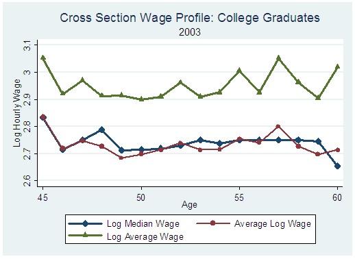
59 Figure 2a Figure 2b

60 Figure 3 Figure 4

61 Figure 5 Figure 6

62 Figure 7 Figure 8

63 Figure 9a Figure 9b

64 Figure 10a Figure 10b

65 Figure 11a Figure 11b

66 Figure 12a Figure 12b

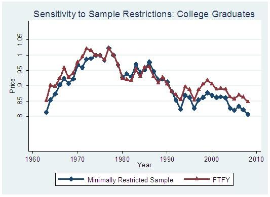
67 Figure A1a Figure A1b

68 Figure A2a Figure A2b

69 Figure A3 Figure A4a