Prioritization for Infrastructure Investment in Transportation

Transcription

1 FREIGHT POLICY TRANSPORTATION INSTITUTE Prioritization for Infrastructure Investment in Transportation Jeremy Sage

2

3 Motivation Why do we (and should we) care about the productivity of Freight Transportation? The Cost of Congestion in Washington State Framework for Determining Truck Freight Benefits and Economic Impacts. Further Exploration of Reliability.

4 Measures of Individual Congestion Yearly delay per auto commuter (hrs) Travel Time Index Planning Time Index (Freeway Only) "Wasted" fuel per auto commuter (gallons) CO2 per auto commuter during congestion (lbs) Congestion cost per auto commuter (2011 dollars) $342 $795 $924 $810 $810 The Nation's Congestion Problem Travel Delay (billion hrs) "Wasted" fuel ($billion) CO2 produced during congestion (billions of lbs) Truck congestion cost ($billion) $27 $27 Congestion cost ($billion) $24 $94 $128 $120 $121 Drawn from TTI s Urban Mobility Report

5 Small = <500,000 Medium = 500,000 to 1 million Large = 1million to 3 million Very Large = >3 million

6 and this is just to operate the trucks. Which brings us to the first FPTI project.

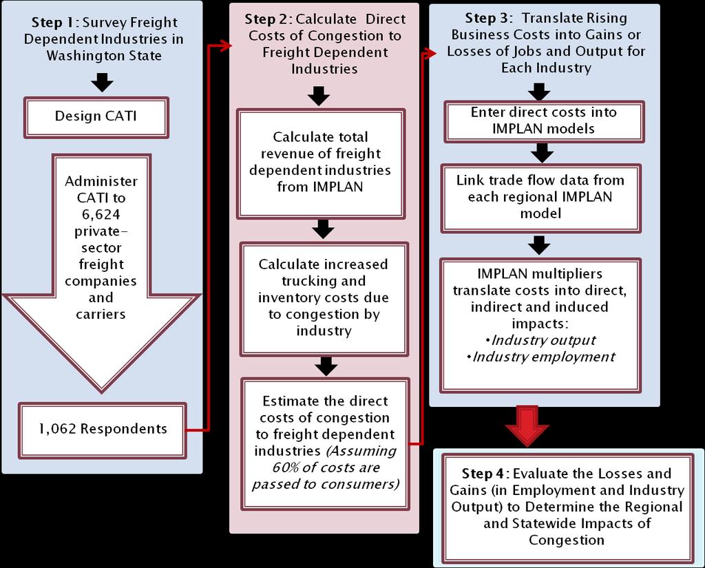
7 Congestion on the urban road network in the United States is estimated to cost the nation in excess of $100 billion, as each and every vehicle using the public roadway system experiences some degree of: Wasted fuel Lost productivity Reduced mobility The cost value is large, but can it inform state level policy? Additional knowledge is needed to understand: How industries are impacted by congestion What their likely response will be to increasing congestion The net impact of these industry responses to the Washington State economy.

8

9 Industry Revenue Agriculture, Forestry, Fishing* $ 14,025,087,392 Mining* $ 1,722,882,632 Construction $ 39,590,105,088 Manufacturing* $ 160,187,755,858 Retail Trade** $ 111,814,709,161 Wholesale Trade** $ 142,323,314,397 Transportation/Warehousing* $ 16,754,995,185 Waste Management $ 3,589,177,344 Calculating Total Revenue: Two modifications from IMPLAN s output values: Subtracted the value of inventory from output to reflect actual sales (*) Adjusted using margins (sales receipts less the cost of the goods sold) to show the total value of the goods sold (**)

10 Industry Inventory Cost Trucking Cost Agriculture, Forestry, Fishing 0.01% 6.00% Mining 0.00% 9.24% Construction 0.04% 8.28% Manufacturing 0.42% 6.04% Retail Trade 0.34% 2.59% Wholesale Trade 0.23% 3.16% Transportation/Warehousing 0.04% 6.51% Waste Management 0.00% 2.86% Inventory Costs (as percent of total revenue) based on need to hold inventory to combat congestion. Trucking Costs represent need for additional trucks, and used in conjunction with reported hourly trucking costs ($55-light, $76-heavy, $59-mixture)

11 Industry Direct Cost of Congestion Agriculture, Forestry, Fishing $ 505,744,651 Mining $ 95,516,613 Construction $ 1,976,338,046 Manufacturing $ 6,208,877,417 Retail Trade $ 1,965,702,587 Wholesale Trade $ 2,894,856,215 Transportation/Warehousing $ 658,471,311 Waste Management $ 61,590,283 Totals nearly $14.4 billion 20% congestion increase 60% cost realization

12

13 Consumers must decease purchases of services and nonfreight dependent goods to pay for the increased costs of freight dependent goods. Household consumption function in IMPLAN was modified to incorporate the spending decrease. Weighted by population and income

14

15 Freight dependent business must increase spending on resources to counteract increased congestion. Congestion as an inefficiency Spending on Insurance and Capital is placed in corresponding IMPLAN industries. Wages modeled as an increase to employee compensation

16

17 Positive Economic Impacts: Industries add employees and assets to combat congestion Negative Economic Impacts: Costs to consumers rise and lead to decreased spending on other industries

18 Positive Economic Impacts: Industries add employees and assets to combat congestion Negative Economic Impacts: Costs to consumers rise and lead to decreased spending on other industries

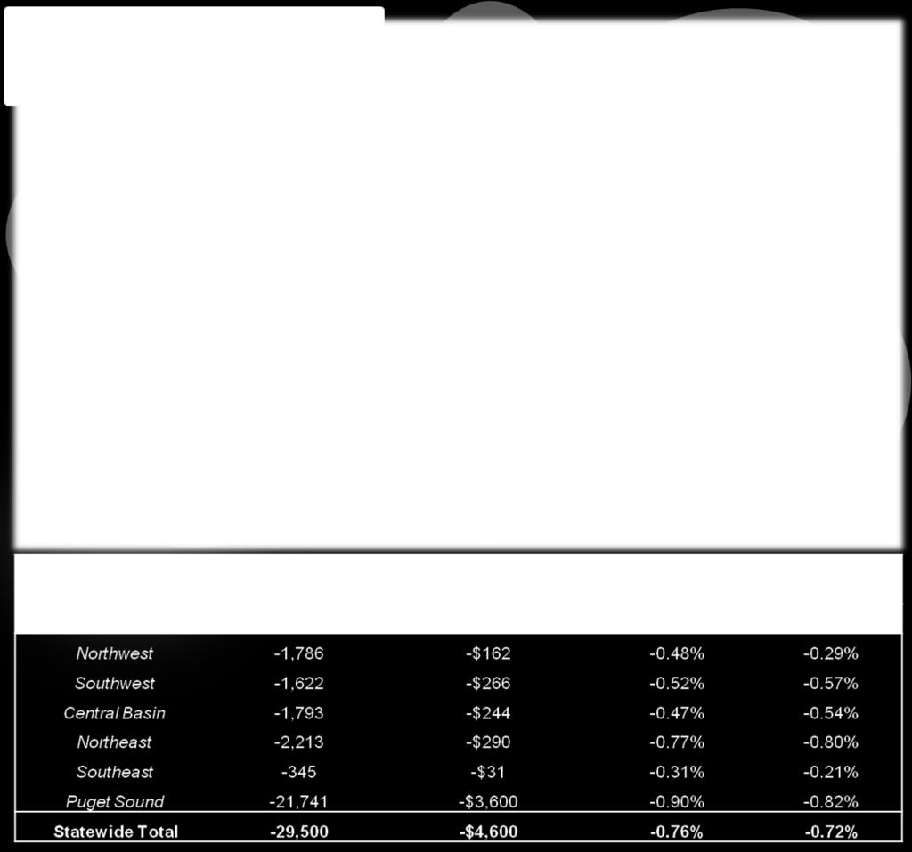
19 Positive Economic Impacts: Industries add employees and assets to combat congestion Negative Economic Impacts: Costs to consumers rise and lead to decreased spending on other industries Industries add 17,831 jobs Industries lose 45,088 jobs Industry output grows $3.03 billion Industry output declines $6.34 billion

20 Positive Economic Impacts: Industries add employees and assets to combat congestion Negative Economic Impacts: Costs to consumers rise and lead to decreased spending on other industries

21 Positive Economic Impacts: Industries add employees and assets to combat congestion Negative Economic Impacts: Costs to consumers rise and lead to decreased spending on other industries

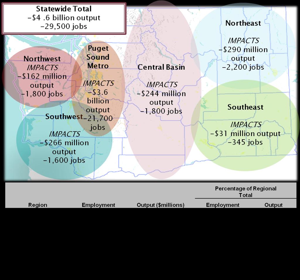
22 Industries incurring additional expenditures (positive impacts) in order to combat congestion Industries suffering from reduced expenditures (negative impacts) Transportation and Information Administrative Services Retail Trade Wholesale Trade Government Manufacturing Management of Companies Mining Health and Social Services Real Estate and Rental Finance and Insurance Accommodation and Food Arts and Entertainment Construction and Utilities Professional and Scientific Educational Services Ag, Forestry, and Fishing

23

24 What do these Findings Suggest for WSDOT s Policies Towards Addressing Congestion on Corridors Used by Trucks? The state s economic vitality and livability depend on reliable, responsible, and sustainable transportation. Congestion causes increased direct transportation costs to freight-dependent industries which translate to increased costs of goods and services to consumers in Washington State. Creates an operational efficiency problem for freight dependent firms: Trip Time Unproductive time in Traffic Productivity resulting in $14 Billion of increased operating costs. These demonstrated economic impacts suggest that WSDOT should prioritize investments that enhance mobility for trucks and freight industries as a way to support the State s goals of a strong economy.

25 Imbedding investment Principles into WSDOT s Moving Washington:

26

27 Truck-freight related benefits should be recognized and acknowledged through quantitative project prioritization process. Most existing project assessment frameworks do not separately evaluate the truck-freight benefits of proposed highway infrastructure projects. Unable to capture full-range of truck-freight related impacts stemming from highway investments. Direct benefits Indirect benefits

28 Propose a transparent methodology for calculating both the direct freight benefits and the larger economic impacts of freight projects. Apply the methodology for projects assessment.

29 Identify benefits Literature review WSDOT current project prioritization process Three technical groups (urban goods movement, global gateway, and rural economies)

30 Direct freight benefits: Truck travel time savings Truck operating cost savings Truck emission changes Economic impacts Employment changes Regional economic output changes

31 Methodology INPUTS Project Specific Data Inputs Travel Demand Model OUTPUTS MODEL FRAMEWORKS Modeling Transportation Related Benefits Benefits from: Travel Time Savings Operating Cost Savings Emissions Changes Modeling Economic Impacts Using Washington State CGE Employment Changes Regional Economic Output CGE: computable general equilibrium model

32 Utilizes Social Accounting Matrices (SAM) from the 2010 IMPLAN data. Aggregate into 20 industrial Sectors: Aggregation Code Freight Dependent Industries Aggregation Code Other Industries AGFOR Agriculture and Forestry INFO Information Services MIN Mining FININS Financial and Insurance UTIL Utilities REAL Real Estate CONST Construction PROTEC Professional and Technical MANUF Manufacturing MANAG Management WTRAD Wholesale Trade ADMIN Administration RTRAD Retail Trade SOCSER Social Services TRAWAR Transportation and Warehousing ARTS Arts and Entertainment TRUCK Transport by Truck FOOD Food Services WMAN Waste Management OTHR Other (Including Government)

33 Create four regional CGE models. 2 Geographic scales Long-Run (LR) and Short-Run (SR) scenarios Model the infrastructure investment as an improvement in technology. Improves the productivity of the transportation system Initiate the CGE through a counterfactual that shifts the industry supply curve: (Cobb-Douglas shown for simplicity) Q=S(K α L 1-α ) Value of the shift is dependent upon the percent change in operating costs to the trucking industry

34 Case Study Interstate-highway widening project 10 mile, 2 lanes each direction. A critical connector for the region and serves approximately 9,000 trucks daily. Freight demand is projected to increase by 30% over the next 10 years. Adding one lane each direction.

35 Case Study -- Transportation Benefits , Thousands of 2010 Dollars Benefit Category VHT reduction 295 hours Truck travel time savings $ 8,704 Truck operating cost savings $14,613 Emission impacts -$5,370 Total $17,947

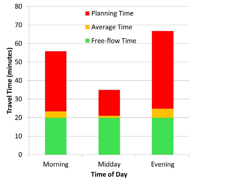
36 Travel Demand Model Benefit Output $ 4,533,563 Spokane County Intermediate Expenditures (TRUCK) $ 139,875,763 Statewide Intermediate Expenditures (TRUCK) $ 1,760,368,000 Change in Truck Transport Productivity -Spokane County 3.24% Change in Truck Transport Productivity -State 0.26% 1

37 Region Initial Employment Level Change in Employment Change in Activity Quantity (%) SR LR SR LR County 264, State 5,647, Price for truck services and regional output sales change: County SR: 1.94% decrease in price and $9.8 million increase in sales LR: 1.67% decrease in price and $28.7 million increase in sales State SR: 0.18% decrease in price and $10.5 million increase in sales LR: 0.14% decrease in price and $22.2 million increase in sales

38 Limitations and Future Work Limitations of using TDMs Limited feedback loops between TDM and Impact Models Future work Freight performance data Enhancing dynamic nature of models

39 Freight Performance Data: Reliability Find a measure of reliability that will be useful and meaningful in a Benefit-Cost (B-C) analysis This requires: Deciding on a measurable definition for travel time reliability. Identifying a value to use for reliability in freight transportation.

40

41 Current Measures of Reliability The mean versus variance approach: uses the mean travel time as well as the standard deviation of travel times. This method is straight forward and relies upon extensive dataset collected from loop detectors, radar detectors, GPS devices, and other technical sensors. The larger the size of the standard deviation from the mean, the lower travel time reliability.

42 Current Measures of Reliability Percentiles: Unreliability is measured and commonly valued as the 95 th percentile travel time. This approach is presented as a numerical difference between the average travel time and a predictable upper deviation from the average. This difference (a real number) is then directly used to monetize the value of unreliability.

43 Current Measures of Reliability Percentiles (cont.): Estimates the time travelers need to plan their trips in order to be on time Buffer time is defined as the 95 th percentile of the travel time distribution minus the mean time. Buffer time index = 95 percent travel time mean travel time mean travel time 100%

44 Current Measures of Reliability Planning Time Index: Estimates the total travel time that should be planned The planning time index differs from the buffer time index in that it considers both recurrent delay and unexpected delay Planning time index = 95 percent travel time Free flow travel time 100%

45 Measure Recommendations If sufficient travel time data is available, e.g. every 5 minute loop detector data Use the buffer time index Represents the extra travel time travelers must to add to ensure on-time arrival. When data is sparse, e.g. low reading frequency GPS data Use the bimodal approach employed by WSDOT Does not require extensive travel time data, but still can examine and classify the reliability based on spot speed data.

46 Identifies if travel time is : Reliably fast, Reliably slow, Unreliable. Travel speeds (in a given time and location segment) follows a mixture of two normal distributions as traffic is composed of two stages: free-flow condition and congestion condition. We can represent truck spot speed distribution by 5 parameters: mean (μ 1 ) & standard deviation (σ 1 ) of congested speed. mean (μ 2 ) & standard deviation (σ 2 ) of free-flow speed. Proportion of the two distribution (α)

47 , 0.2, and 0.75 V f

48 Probability Density μ σ α μ σ Speed Normal Mixture Night (12 AM 6 AM) AM Peak (6 AM 9 AM) If No Yes 2

49 Conclusion A quantitative and transparent methodology capturing freight benefits can be used for freight project impacts assessment and project prioritization. Industrial base of a geographical region significantly impacts model outputs. The inclusion of a defendable and quantifiable reliability measure will be a significant contribution to the understanding of freight performance measures.

50 For more Information: