Analysis of Process Models: Introduction, state space analysis and simulation in CPN Tools. prof.dr.ir. Wil van der Aalst

Transcription

1 Analysis of Process Models: Introduction, state space analysis and simulation in CPN Tools prof.dr.ir. Wil van der Aalst

2 What is a Petri net? A graphical notion A mathematical notion A programming notion (model = picture?) (model = graph?) (model = program?) A solver independent medium Starting point for a variety of analysis approaches ANA-1

3 Analysis Operational process Model Information System Analysis is typically modeldriven to allow e.g. what-if questions. Models of both operational processes and/or the information systems can be analyzed. Types of analysis: validation verification performance analysis ANA-2

4 Three types of analysis techniques 1. Reachability/coverability graph 2. Structural techniques Place and transition invariants Marking equation Traps, siphons, etc. 3. Simulation Each can be applied to both classical and high-level Petri nets. Nevertheless, for the second we restrict ourselves to classical Petri nets. Mapping technique/use: reachability graph (validation, verification) invariants (validation, verification) simulation (validation, performance analysis) ANA-3

5 Informal introduction... ANA-4

6 Examples of generic questions given a marked Petri net terminating it has only finite occurrence sequences deadlock-free each reachable marking enables a transition live each reachable marking enables an occurrence sequence containing all transitions bounded each place has an upper bound that holds for all reachable markings 1-safe 1 is a bound for each place p reversible m 0 is reachable from each reachable marking, i.e., the initial marking is a so-called home marking. ANA-5

7 Reachability graph rg1 rg2 (0,0,1,1,0,0,0) (1,0,0,0,0,1,0) g1 g2 r1 go1 x go2 r2 (1,0,0,1,0,0,1) o1 o2 (0,1,0,1,0,0,0) (1,0,0,0,1,0,0) or1 or2 Five reachable states. Traffic lights are safe! ANA-6

8 Alternative notation terminating it has only finite occurrence sequences deadlock-free rg1 rg2 each reachable marking enables a transition live r1 go1 bounded g1 each reachable marking enables an occurrence sequence containing all transitions x each place has an upper bound that holds for all reachable markings or1 or2 m 0 is reachable from each reachable go2 o1 o2 1-safe 1 is a bound for each place p reversible marking, i.e., the initial marking is a so-called home marking. g2 r2 o1+r2 g1+r2 r1+r2+x r1+o2 r1+g2 ANA-7

9 Reachability graph (2) Graph containing a node for each reachable state. Constructed by starting in the initial state, calculate all directly reachable states, etc. Expensive technique. Only feasible if finitely many states (otherwise use coverability graph). Difficult to generate diagnostic information. ANA-8

10 Infinite reachability graph rg1 rg2 g1 g2 r1 go1 x go2 r2 or1 o1 or2 o2 Therefore tools use a coverability graph which is always finite! ANA-9

11 Exercise: Construct reachability graph free wait enter before make_picture after leave gone occupied ANA-10

12 Exercise: Dining philosophers 4 philosophers sharing 4 chopsticks: A philosopher is either in state eating or thinking and needs two chopsticks to eat. Model as a Petri net and construct reachability graph. D:\www\wvdaalst\workflowcourse\examples\philosopher4.swf ANA-11

13 See also: D:\www\wvdaalst\workflowcourse\examples\philosopher4_RG.swf ANA-12

14 Analysis in CPN Tools Only state-space analysis, i.e., no invariants. Generate report in text file. State-space visualization from version 2.2. Steps: 1. Enter the State Space Tool (to generate ML code) 2. Calculating the state space 3. Calculating the SCC graph (to calculate home states and fairness) 4. Save/view state space report ANA-13

15 Example ANA-14

16 Create report PAGE 15

17 Report (1) CPN Tools state space report for: /cygdrive/d/courses/bis-2011/cpn files/voting-bank-etc/bank.cpn Report generated: Sun Mar 27 14:01: Statistics State Space Nodes: 24 Arcs: 44 Secs: 0 Status: Full Scc Graph Nodes: 24 Arcs: 44 Secs: 0 ANA-16

18 Report (2) Boundedness Properties Best Integer Bounds Upper Lower main'database main'deposit main'withdraw Best Upper Multi-set Bounds main'database 1 1`(1,0)++ 1`(2,(~5))++ 1`(2,(~1))++ 1`(2,0)++ 1`(2,3)++ 1`(2,4)++1`(2,7)++1`(2,8)++1`(2,11)++1`(2,12)++1`(2,15)++1`(2,16)+1`(2,20)++1 `(3,(~9))++1`(3,0) main'deposit 1 5`(2,4) main'withdraw 1 1`(2,5)++1`(3,9) Best Lower Multi-set Bounds main'database 1 1`(1,0) main'deposit 1 empty main'withdraw 1 empty ANA-17

19 Report (3) Home Markings [24] Liveness Properties Dead Markings [24] Dead Transition Instances None Live Transition Instances None Fairness Properties No infinite occurrence sequences. ANA-18

20 ANA-19

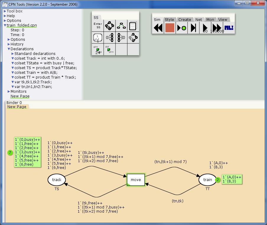
21 State Space Nodes: 28 Arcs: 42 Secs: 0 Status: Full Scc Graph Nodes: 1 Arcs: 0 Secs: 0 Boundedness Properties Best Integer Bounds Upper Lower New_Page'track New_Page'train ANA-20

22 Home Properties Home Markings All Liveness Properties Dead Markings None Dead Transition Instances None Live Transition Instances All Fairness Properties New_Page'move 1 Impartial ANA-21

23 Another example ANA-22

24 Report (1) CPN Tools state space report for: C:\Program Files\CPN Tools\Samples\DiningPhilosophers\DiningPhilosophers.cpn Report generated: Thu Nov 02 10:42: Statistics State Space Nodes: 11 Arcs: 30 Secs: 0 Status: Full Scc Graph Nodes: 1 Arcs: 0 Secs: 0 ANA-23

25 Report (2) Boundedness Properties Best Integer Bounds Upper Lower Page'Eat Page'Think Page'Unused_Chopsticks Best Upper Multi-set Bounds Page'Eat 1 1`ph(5) Page'Think 1 1`ph(5) Page'Unused_Chopsticks 1 1`ph(1)++ 1`ph(2)++ 1`ph(3)++ 1`ph(4)++ 1`ph(1)++ 1`ph(2)++ 1`ph(3)++ 1`ph(4)++ 1`cs(1)++ 1`cs(2)++ 1`cs(3)++ 1`cs(4)++ 1`cs(5) Best Lower Multi-set Bounds Page'Eat 1 Page'Think 1 Page'Unused_Chopsticks 1 empty empty empty ANA-24

26 Report (3) Home Properties Home Markings All Liveness Properties Dead Markings None Dead Transition Instances None Live Transition Instances All strongest fairness property, i.e., there are infinite firing sequences and in each infinite firing sequence t occurs infinitely often Fairness Properties Page'Put_Down_Chopsticks 1 Impartial Page'Take_Chopsticks 1 Impartial ANA-25

27 Fairness properties Are only relevant if there are Infinite Firing Sequences (IFS), otherwise CPN Tools reports: "no infinite occurrence sequences". Given a transition t it is often desirable that t appears infinitely often in an IFS. Properties reported by CPN Tools t is impartial: t occurs infinitely often in every IFS. t is fair: t occurs infinitely often in every IFS where t is enabled infinitely often. t is just: t occurs infinitely often in every IFS where t is continuously enabled from some point onward No fairness: not just, i.e., there is an IFS where t is continuously enabled from some point onward and does not fire anymore ANA-26

28 Example Fairness Properties main1'a 1 Just main1'b 1 Just main1'c 1 Impartial ANA-27

29 Example Fairness Properties main2'x 1 No Fairness main2'y 1 No Fairness ANA-28

30 Example Fairness Properties main3't1 1 Fair main3't2 1 No Fairness main3't3 1 No Fairness main3't4 1 No Fairness main3't5 1 No Fairness main3't6 1 Just ANA-29

31 Exercise t1 p1 t4 p2 p4 p3 t2 Indicate for each transition whether it is impartial, fair, or just (or satisfies no fairness property) t3 ANA-30

32 t1, t2, and t3 are all impartial because it is not possible to construct an infinite firing sequence where not all of these transitions appear infinitely often. If one stops executing one of these transitions, the system will block after a while. t1 p1 t4 p2 p4 p3 t2 t4 has no fairness as it is possible to construct an infinite firing sequence where t4 remains enabled but never fires. t3 ANA-31

33 Simulation Most widely used analysis technique. From a technical point of view just a "walk" in the reachability graph. By making many "walks" (in case of transient behavior) or a very "long walk" (in case of steadystate) behavior, it is possible to make reliable statements about properties/ performance indicators. Used for validation and performance analysis. Cannot be used to prove correctness! ANA-32

34 Stochastic process Simulation of a deterministic system is not very interesting. Simulation of an untimed system is not interesting. In a timed and non-deterministic system, durations and probabilities are described by some probability distribution. In other words, we simulate a stochastic process! CPN allows for the use of distributions using some internal random generator. ANA-33

35 Uniform distribution probability density function (PDF) cumulative distribution function (CDF) ANA-34

36 Negative exponential distribution ANA-35

37 Normal distribution ANA-36

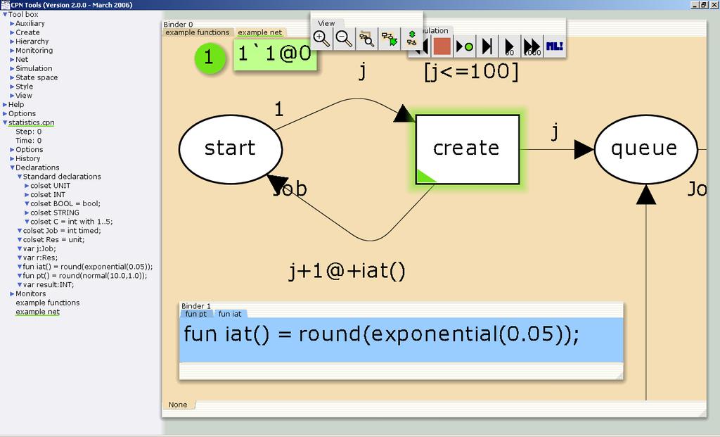
38 Distributions in CPN Tools There is standard library with stochastic functions: uniform(a:real, b:real) : real exponential(r:real) : real normal(n:real, v:real) : real erlang (n:int, r:real) : real Etc. A nice additional function is also C.ran() which returns a randomly selected element of finite color set C, e.g., color C = int with 1..5; fun select1to5() = C.ran() returns a number between 1 and 5 ANA-37

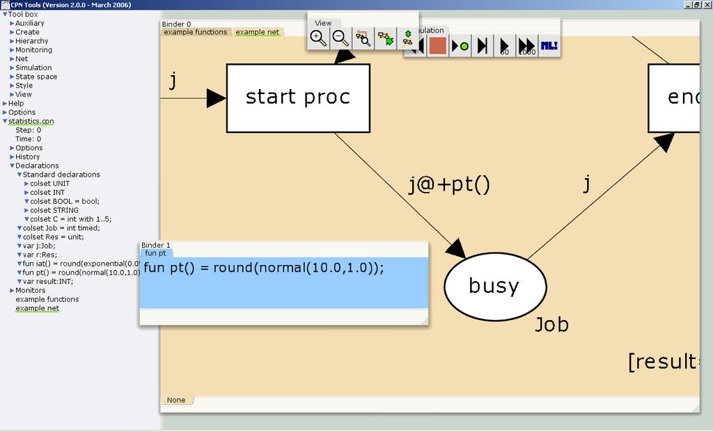
39 Example color BT = unit; color Dice = int with 1..6; var d : Dice; () () Dice.ran() trigger BT () throw_dice outcome Dice or even simpler d throw_dice outcome Dice ANA-38

40 Example(2) trigger color INT = int; color TINT = int timed; color Dice = int with 1..6; color Delay = int with 0..99; 0 x throw_dice Dice.ran() TINT (x+1)@+(delay.ran()) outcome Dice ANA-39

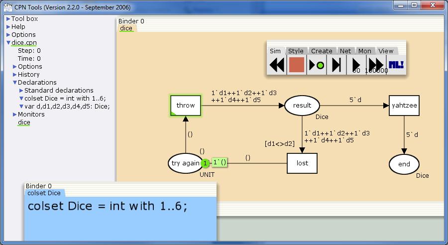
41 Yahtzee ANA-40

42 After 2055 times throwing the dices five 4 s ANA-41

43 Examples ANA-42

44 Example ANA-43

45 ANA-44

46 ANA-45

47 alternative notation [b]%v = if b then 1`v else empty [result =1]%j [result =0]%j ANA-46

48 Adding hierarchy ANA-47

49 Example revisited ANA-48

50 Subruns and confidence intervals A single run does not provide information about reliability of results. Therefore, multiple runs or one run cut into parts: subruns. If the subruns are assumed to be mutually independent, one can calculate a confidence interval, e.g., the flow time is with 95% confidence within the interval 5.5+/-0.5 (i.e. [5,6]). ANA-49

51 Two possible settings Steady-state analysis (I) Steady-state analysis (II) ANA-50

52 More on calculating confidence intervals average minimum maximum variance utilization weighted average ANA-51

53 is not the same as although the average over the subrun results is the same (5.7) ANA-52

54 "low level" measurements aggregation per subrun (average, min, max, variance, etc.) subruns = 11 average = 5.7 standard deviation = 0.21 confidence = 0.9 confidence interval = [ , ] = [5.58,5.82] ANA-53

55 Using monitors in CPN Tools ANA-54

56 Example of a simulation model Gas station with one pump and space for 4 cars (3 waiting and 1 being served). Service time: uniform distribution between 2 and 5 minutes. Poisson arrival process with mean time between arrivals of 4 minutes. If there are more than 3 cars waiting, the "sale" is lost. Questions: flow time, waiting time, utilization, lost sales, etc. ANA-55

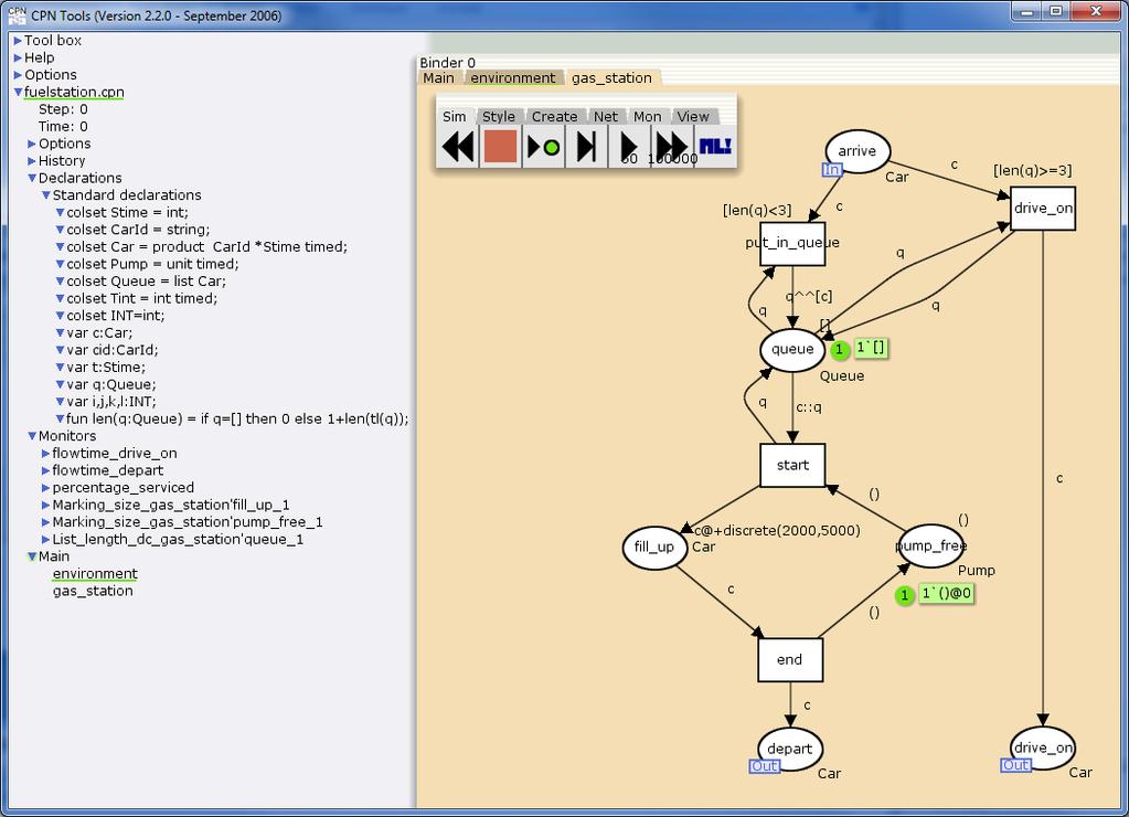
57 Top-level page: main color Car = string HS arrive Car HS environment gas_station drive_on Car depart Car ANA-56

58 Subpage gas_station arrive In Car [len(q)<3] c c [len(q)>=3] color Car = string; color Pump = unit; color TCar = Car timed; color Queue = list Car; var c:car; var q:queue; fun len(q:queue) = if q=[] then 0 else 1+len(tl(q)); put_in_queue q queue q start q^^[c] [] Queue c::q q q drive_on c@+uniform(2,5) () c pump_free () fill_up TCar Pump c () end c Out Out depart Car drive_on Car ANA-57

59 Interesting performance indicators: Calculation of flow time (average, variance, maximum, minimum, service level, etc.). Calculation of waiting times (average, variance, maximum, minimum, service level, etc.). Calculation of lost sales (average). Probability of no space left. Probability of no cars waiting. ANA-58

60 Alternatives arrive In Car [len(q)<3] c c [len(q)>=3] color Car = string; color Pump = unit; color TCar = Car timed; color Queue = list Car; var c:car; var q:queue; fun len(q:queue) = if q=[] then 0 else 1+len(tl(q)); put_in_queue q queue q start q^^[c] [] Queue c::q q q drive_on Model the following alternatives: 6 waiting spaces 2 pumps 1 faster pump c@+uniform(2,5) () pump_free fill_up TCar c () end c () Pump c Out Out depart Car drive_on Car ANA-59

61 Experiments (note time dimension * 1000; not needed in CPN Tools Version 3) ANA-60

62 ANA-61

63 monitors ANA-62

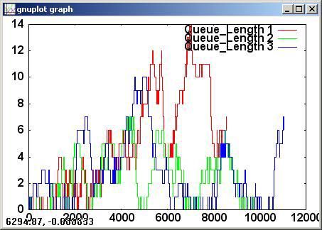
64 Number of cars being served ANA-63

65 Number of pumps free ANA-64

66 Length of queue ANA-65

67 Flow time for cars not served ANA-66

68 Flow time for cars that have been served ANA-67

69 Percentage of cars served ANA-68

70 Average flow is time Just one run ANA-69

71 Subruns in CPN Tools X 10 CPN'Replications.nreplications 10 ANA-70

72 Average queue length [0.878,0.906] Average # pumps busy [0.794,0.801] Average # pumps free [0.198,0.206] ANA-71

73 Average flow time [7.352,7.460] Average fraction served [0.910,0.915] ANA-72

74 Results Average flow time Average fraction served Base case [7.352,7.460] [0.910,0.915] PAGE 73

75 2 pumps ANA-74

76 Average queue length [0.105,0.111] Average # pumps busy [0.867,0.878] Average # pumps free [1.122,1.133] ANA-75

77 Average flow time [3.916,3.944] Average fraction served[0.996,0.997] ANA-76

78 Results Average flow time Average fraction served Base case [7.352,7.460] [0.910,0.915] Two pumps [3.916,3.944] [0.996,0.997] PAGE 77

79 6 places to queue ANA-78

80 Average queue length [1.691,1.770] Average # pumps busy [0.841,0.851] Average # pumps free [0.149,0.159] ANA-79

81 Average flow time [10.518,10.774] Average fraction served [0.966,0.970] ANA-80

82 Results Average flow time Average fraction served Base case [7.352,7.460] [0.910,0.915] Two pumps [3.916,3.944] [0.996,0.997] Six places [10.518,10.774] [0.966,0.970] PAGE 81

83 faster pump [2-5] => [ ] ANA-82

84 Average queue length [0.378,0.399] Average # pumps busy [0.595,0.605] Average # pumps free [0.395,0.405] ANA-83

85 Average flow time [4.000,4.065] Average fraction served [0.976,0.979] ANA-84

86 Results Average flow time Average fraction served Base case [7.352,7.460] [0.910,0.915] Two pumps [3.916,3.944] [0.996,0.997] Six places [10.518,10.774] [0.966,0.970] Faster pump [4.000,4.065] [0.976,0.979] PAGE 85

87 Insights obtained from simulation Adding a pump significantly reduces the flow time (from approx. 7.4 to approx. 3.9 minutes) and reduces the percentage not served (from approx. 9% to approx. 1%). Adding more waiting places significantly increases the flow time (from approx. 7.4 to approx minutes) but reduces the percentage not served (approx. 9% to approx. 3%). Installing a faster pump significantly reduces the flow time (from approx. 7.4 to approx. 4.0 minutes) and reduces the percentage not served (from approx. 9% to approx. 3%). ANA-86

88 Analytical models versus Simulation models ANA-87

89 Example: M/M/1 queue arrival rate λ (average interarrival time = 1/λ) service rate μ (average interarrival time = 1/μ) utilization ρ = λ/μ average nof cases in system L = ρ/(1 - ρ) average flow time S = 1/(μ-λ) Example: λ = 1/100 and μ = 1/50 ρ = 0.5 L = 1 S = 100 ANA-88

90 M/M/1 queue λ = 1/100 μ = 1/50 ρ = 0.5 L = 1 S = 100 λ = 1/100 μ = 1/80 ρ = 0.8 L = 4 S = 400 flow time utilization λ = 1/100 μ = 1/99 ρ = 0.99 L = 99 S = 9900 ANA-89

91 CPN model with monitors ANA-90

92 Creating monitors ANA-91

93 Single run ANA-92

94 CPN'Replications.nreplications 10 90% [ , ] λ = 1/100 μ = 1/50 ρ = 0.5 L = 1 S = 100 ANA-93

95 CPN'Replications.nreplications 10 λ = 1/100 μ = 1/80 ρ = 0.8 L = 4 S = 400 ANA-94

96 CPN'Replications.nreplications 10 λ = 1/100 μ = 1/99 ρ = 0.99 L = 99 S = 9900 Note deviations. Why? ANA-95

97 Conclusion analysis Operational process Model Information System Analysis is typically modeldriven to allow e.g. what-if questions. Models of both operational processes and/or the information systems can be analyzed. Types of analysis: validation (interactive simulation/gaming) verification (state-space analysis, place and transition invariants, siphons, traps, etc.) performance analysis (simulation) ANA-96