Queues (waiting lines)

Transcription

1 Queues (waiting lines)

2 Non-people queues Great inefficiencies also occur because of other kinds of waiting than people standing in line. For example, making machines wait to be repaired may result in lost production. Vehicles (including ships and trucks) that need to wait to be unloaded may delay subsequent shipments. Airplanes waiting to take off or land may disrupt later travel schedules. 2

3 Non-people queues Delays in telecommunication transmissions due to saturated lines may cause data glitches. Causing manufacturing jobs to wait to be performed may disrupt subsequent production. Delaying service jobs beyond their due dates may result in lost future business. 3

4 Queueing Theory Queueing theory is the study of waiting in all these various forms. It uses queueing models to represent the various types of queueing systems (systems that involve queues of some kind) that arise in practice. 4

5 Queueing Theory Formulas for each model indicate how the corresponding queueing system should perform, including the average amount of waiting that will occur, under a variety of circumstances. 5

6 Queueing Models Therefore, these queueing models are very helpful for determining how to operate a queueing system in the most effective way. Providing too much service capacity to operate the system involves excessive costs. But not providing enough service capacity results in excessive waiting and all its unfortunate consequences. 6

7 Queueing Models The models enable finding an appropriate balance between the cost of service and the amount of waiting. 24/02/ Ileana Castillo, Ph.D.

8 Queueing Process 24/02/ Ileana Castillo, Ph.D.

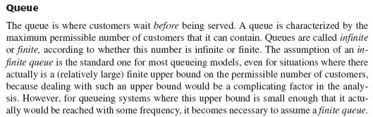
9 the infinite case, this assumption is often made. 9

10 The statistical pattern by which customers are generated over time must also be specified. The common assumption is that they are generated according to a Poisson process; i.e., the number of customers generated until any specific time has a Poisson distribution. This case is the one where arrivals to the queueing system occur randomly but at a certain fixed mean rate, regardless of how many customers already are there (so the size of the input source is infinite). 10

11 An equivalent assumption is that the probability distribution of the time between consecutive arrivals is an exponential distribution. The time between consecutive arrivals is referred to as the interarrival time. Any unusual assumptions about the behavior of arriving customers must also be specified. One example is balking, where the customer refuses to enter the system and is lost if the queue is too long. 11 Ileana Castillo, Ph.D.

12 12

13 FCFS LCFS SIRO: Service in random order GD: General queue discipline 13

14 14

15 15

16 The time elapsed from the commencement of service to its completion for a customer at a service facility is referred to as the service time. A model of a particular queueing system must specify the probability distribution of service times for each server (and possibly for different types of customers), although it is common to assume the same distribution for all servers. 16

17 The service-time distribution that is most frequently assumed in practice (largely because it is far more tractable than any other) is the exponential distribution Other important service-time distributions are the degenerate distribution (constant service time) and the Erlang (gamma) distribution 17

18 18

19 Kendall-Lee Notation:1/2/3 M M s 19

20 In these cases, the notation for the queueing model in the previous slide would be: M M s, M D s M Ek s, M G s 24/02/2011 Ileana Castillo, Ph.D. 20

21 21

22 Ileana Castillo, Ph.D. 22

23 23

24 Certain notation also is required to describe steady-state results. When a queueing system has recently begun operation, the state of the system (number of customers in the system) will be greatly affected by the initial state and by the time that has since elapsed. The system is said to be in a transient condition 24

25 However, after sufficient time has elapsed, the state of the system becomes essentially independent of the initial state and the elapsed time (except under unusual circumstances). The system has now essentially reached a steady-state condition, where the probability distribution of the state of the system remains the same (the steadystate or stationary distribution) over time. 25

26 Queueing theory has tended to focus largely on the steady-state condition, partially because the transient case is more difficult analytically. The following notation assumes that the system is in a steady-state condition: 26

27 27

28 The exponential distribution 28

29 29

30 Interarrival times = = = = = = = = + 30

31 31

32 Importance of Property 2 If we want to know the probability distribution of the time until the next arrival, then it does not matter how long it has been since the last arrival 32

33 33

34 34

35 Ejemplo del Winston 35 Escuela de Ingeniería Industrial y de Sistemas

36 Ejemplo λ λ = = = 36 Escuela de Ingeniería Industrial y de Sistemas

37 Ejercicios 37 Escuela de Ingeniería Industrial y de Sistemas

38 Ejercicios 38 Escuela de Ingeniería Industrial y de Sistemas

39 R: a) , b) , c)

40 References Chase, Jacobs & Aquilano. (2005). Administración de la Producción y Operaciones, 10 a Edición, México: McGraw-Hill. Hillier, F.S. and Lieberman, G.J. (2006). Introducción a la Investigación de Operaciones. 8 a edición, México: McGraw Hill. Winston, W.L. (2005). Investigación de Operaciones. 4 a edición. México: Thomson. Anderson, D.R., Sweeney, D.J. y Williams, T.A. (2004). Métodos cuantitativos para los negocios. 9ª edición. México: Thomson. 40