Calculating Absolute Rate Differences and Relative Rate Ratios in SAS/SUDAAN and STATA. Ashley Hirai, PhD May 20, 2014

Transcription

1 Calculating Absolute Rate Differences and Relative Rate Ratios in SAS/SUDAAN and STATA Ashley Hirai, PhD May 20, 2014

2 Outline Importance of absolute and relative measures Problems with odds ratios as a relative measure Estimating adjusted Rate Differences (RDs) and Rate Ratios (RRs) in SAS and STATA Additive and multiplicative interactions

3 Measures of Association Differences between groups (person, place, time) in an outcome can be assessed by simple differences (subtraction) or ratios (division) Absolute risk/rate difference (attributable risk) = P(outcome) 1 P(outcome) 2 Relative risk/rate ratio = P(outcome) 1 P(outcome) 2

4 Absolute Measures Absolute risk/prevalence differences carry advantage of assessing actual impact Potentially avertable or excess cases (attributable fractions) Number needed to treat (cost-benefit) Decomposition analyses (Kitagawa, PPOR) However, can be difficult to compare strength of association across risk factors, outcomes, etc

5 Relative Measures of Association Help to control or standardize assessments across indicators or person/place/time to compare strength or magnitude of association More typically used in etiologic studies However, can be misleading A doubling of risk sounds dramatic, RR=2 1% to 2%, RR=2 but absolute increase is 1%, still very unlikely to have outcome Y 30% to 60%, RR=2 but absolute increase is 30%, now more likely than not to have outcome Y

6 Absolute and Relative Measures Provide unique information and are complementary When evaluating the effect of a single factor within one group or time period, there is qualitative concordance A positive RD will correspond with RR>1 A negative RD will correspond with RR<1 However, indicators can be inconsistent when comparing the effect in two groups or time periods (interactions)

7 2) Ratio Measures Can t Be Easily Compared

8 = = = 28.8 per 100,000 population Black White = 10.3

9 Healthy People Decline in both absolute and relative differences is best evidence of progress in disparity elimination Relative measures of disparity are primary indicator of progress because they adjust for changes in the level of the reference point over time Relative measures also have advantage of adjusting for differences in reference point when comparisons are made across objectives Keppel KG, Pearcy JN, Klein RJ. Measuring progress in Healthy People Healthy People 2010 Stat Notes Sep;(25):1-16.

10 Additive versus Multiplicative Interaction Multiplicative interaction may be an extreme standard; cases where multiplicative interaction is not present but additive is with important public health implications Stroke Incidence per 1,000 Smoke - Smoke + Risk Difference Relative Risk OC Pill OC Pill Joint effects exhibit additive interaction: increase of 50 cases versus expected 30 Multiplicative interaction not present, 3*2=6, RR of 6 expected and observed

11 Why both absolute and relative measures matter Absolute measures quantify actual risks and number affected Necessary to evaluate/interpret the meaning of a given RR Relative measures allow standardized comparisons across groups, time periods, indicators Lack of correspondence for interactions creates controversy of which is better but they provide complementary information

12 Problems with the Odds Ratio and why it should be avoided Non-intuitive, difficult to communicate/interpret correctly Exaggeration of relative risk for common outcomes Breastfeeding, obesity, medical home Not collapsible across strata; crude OR < average of stratum-specific OR can lead to apparent (negative) confounding when none exists or positive confounding not to be detected

13 RR versus OR RR = P2 P1 OR = P2 (1 P2) P1 (1 P1) = P2 P1 *(1 P1) (1 P2) = RR*(1 P1) (1 P2) OR RR = (1 P1) (1 P2) For RRs>1, a doubling can occur When P1 is small and P2 is much greater (high effect size) For p1=.1, p2=(.1+1)/2=.55 ; RR=5.5; OR=11 As P1 increases, the distance to P2 doesn t have to be as large (high prevalence) For p1=.5, p2=(.5+1)/2=0.75; RR=1.5; OR=3 Basically, high prevalence in at least one strata

14 Estimation Options for Risk Differences and Risk Ratios Showing code in SAS and STATA Examples with non-sampled and complex survey data Acknowledgement: Jay Kaufman, PhD McGill University

15 Model Options 1) Linear Probability Model 2) Generalized Linear Model (Binomial, Poisson) 3) Logistic Model (probability conversions)

16 Simple Data Example Birth certificate data Outcome: Preterm Birth (<37 weeks gestation) Covariates: Smoking, race/ethnicity, maternal age Example applies to cohort or cross-sectional data generally and population-level (nonsampled) or simple random samples

17 1) Linear Probability Model: Advantages: Disadvantages: very easy to fit single uniform estimate of RD economists will love you possible to get impossible estimates does not directly estimate RR biostatisticians will hate you Fit an OLS linear regression on the binary outcome variable: Pr(Y=1 X=x) = β 0 + β 1 X Note: Homoskedasticity assumption cannot be met, since variance is a function of p. Therefore, use robust variance.

18 Linear Probability Model (OLS) proc surveyreg order=formatted; class racex; model ptb = smoke mager mager*mager racex /clparm solution; run; Regression Analysis for Dependent Variable ptb Estimated Regression Coefficients Standard 95% Confidence Parameter Estimate Error t Value Pr > t Interval Intercept < smoke < mager < mager*mager < racex a Non-Hispanic Black < racex b Hispanic < racex c Other racex d Non-Hispanic White Adjusted RD for smoking= (95% CI 0.028, 0.031)

19 regress ptb smoke c.mager##c.mager i.racex, vce(robust) cformat(%6.4f) Linear regression Number of obs = F( 6, ) = Prob > F = R-squared = Root MSE = Robust ptb Coef. Std. Err. t P> t [95% Conf. Interval] smoke , mager , c.mager# c.mager , racex , , , _cons , Adjusted RD for smoking = (95% CI: , )

20 2) Generalized Linear Model: Advantages: Disadvantages: single uniform estimate biostatisticians will love you can be difficult to fit still possible to get impossible values Fit a GLM with a binomial or Poisson distribution For RD: identity link For RR: log link g[pr(y=1 X=x)] = β 0 + β 1 X Generally fit Poisson when binomial fails to converge, must use robust standard errors due to binary data Spiegelman D, Hertzmark E. Easy SAS calculations for risk or prevalence ratios and differences. Am J Epidemiol 2005 Aug 1;162(3):

21 Binomial Model Risk Difference, Identity Link proc genmod descending; class racex/order=formatted; model ptb = smoke mager mager*mager racex / dist=bin link=identity; format racex racex.; run; Analysis Of Maximum Likelihood Parameter Estimates Standard Wald 95% Confidence Wald Parameter DF Estimate Error Limits Chi-Square Intercept smoke mager mager*mager racex a Non-Hispanic Black racex b Hispanic racex c Other racex d Non-Hispanic White Scale Adjusted RD for smoking = (95% CI , )

22 glm ptb smoke c.mager##c.mager i.racex, fam(b) lin(ident) binreg ptb smoke c.mager##c.mager i.racex, ml rd Generalized linear models No. of obs = Optimization : ML Residual df = Scale parameter = 1 Deviance = (1/df) Deviance = Pearson = (1/df) Pearson = Variance function: V(u) = u*(1-u) [Bernoulli] Link function : g(u) = u [Identity] Log likelihood = OIM ptb Coef. Std. Err. z P> z [95% Conf. Interval] smoke , mager , c.mager# c.mager , racex , , , _cons , Coefficients are the risk differences.

23 Binomial Model Risk Ratio, Log Link proc genmod descending; class racex/order=formatted; model ptb = smoke mager mager*mager racex / dist=bin link=log; estimate 'RR smoke' smoke 1; format racex racex.; run; Standard Wald 95% Confidence Wald Parameter DF Estimate Error Limits Chi-Square Intercept smoke mager mager*mager racex a Non-Hispanic Black racex b Hispanic racex c Other racex d Non-Hispanic White Scale Contrast Estimate Results Mean Mean L'Beta Standard L'Beta Label Estimate Confidence Limits Estimate Error Alpha Confidence Limits RR smoke Adjusted RR for smoking = 1.31 (95% CI 1.30, 1.33)

24 glm ptb smoke c.mager##c.mager i.racex, fam(b) lin(log) eform binreg ptb smoke c.mager##c.mager i.racex, ml rr Generalized linear models No. of obs = Optimization : ML Residual df = Scale parameter = 1 Deviance = (1/df) Deviance = Pearson = (1/df) Pearson = Variance function: V(u) = u*(1-u) [Bernoulli] Link function : g(u) = ln(u) [Log] AIC = Log likelihood = BIC = -2.93e+07 OIM ptb Risk Ratio Std. Err. z P> z [95% Conf. Interval] smoke mager c.mager# c.mager racex Adjusted RR for smoking = 1.31 (95% CI: 1.30, 1.33)

25 Additive Interaction proc genmod; class id smoke racex/param=ref ref=first; model ptb = smoke mager mager*mager racex smoke*racex/ dist=bin link=id; estimate 'smoking among NH Black' smoke 1 smoke*racex 1 0 0; format racex racex.; run; Analysis Of Maximum Likelihood Parameter Estimates Standard Wald 95% Confidence Wald Parameter DF Estimate Error Limits Chi-Square Pr > ChiSq Intercept <.0001 smoke <.0001 mager <.0001 mager*mager <.0001 racex a Non-Hispanic Black <.0001 racex b Hispanic <.0001 racex c Other <.0001 racex d Non-Hispanic White smoke*racex a Non-Hispanic Black smoke*racex b Hispanic smoke*racex c Other smoke*racex d Non-Hispanic White Scale Contrast Estimate Results Mean Mean L'Beta Standard L'Beta Chi- Label Estimate Confidence Limits Estimate Error Alpha Confidence Limits Square Pr > ChiSq smoking among NH Black <.0001 Effect of smoking greater among Black than White women

26 glm ptb smoke c.mager##c.mager i.racex smoke##i.racex, fam(bin) lin(id) binreg ptb smoke c.mager##c.mager i.racex, ml rd lincom smoke + 1.smoke#2.racex // smoking for Black women OIM ptb Coef. Std. Err. z P> z [95% Conf. Interval] smoke mager c.mager# c.mager e racex smoke#racex _cons Coefficients are the risk differences. ( 1) smoke + 1.smoke#2.racex = 0 ptb Coef. Std. Err. z P> z [95% Conf. Interval] (1)

27 Multiplicative Interaction proc genmod; class racex/order=formatted; model ptb = smoke mager mager*mager racex smoke*racex/ dist=bin link=log; estimate 'smoking among White' smoke 1; estimate 'smoking among NH Black' smoke 1 smoke*racex 1 0 0; format racex racex.; Run; Analysis Of Maximum Likelihood Parameter Estimates Standard Wald 95% Confidence Wald Parameter DF Estimate Error Limits Chi-Square Pr > ChiSq Intercept <.0001 smoke <.0001 mager <.0001 mager*mager <.0001 racex a Non-Hispanic Black <.0001 racex b Hispanic <.0001 racex c Other racex d Non-Hispanic White smoke*racex a Non-Hispanic Black smoke*racex b Hispanic smoke*racex c Other smoke*racex d Non-Hispanic White Scale Contrast Estimate Results Mean Mean Label Estimate Confidence Limits smoking among White ssmoking among NH Black Additive but not multiplicative interaction

28 glm ptb smoke c.mager##c.mager i.racex smoke##i.racex, fam(bin) lin(log) binreg ptb smoke c.mager##c.mager i.racex, ml rr lincom smoke, eform // smoking for White lincom smoke + 1.smoke#2.racex, eform //smoking for Black OIM ptb Coef. Std. Err. z P> z [95% Conf. Interval] smoke mager c.mager# c.mager racex smoke#racex _cons ptb exp(b) Std. Err. z P> z [95% Conf. Interval] Smoking for White Smoking for Black

29 If Binomial fails to converge, try starting with a negative intercept proc genmod data=ahs.sample_10; class racex/order=formatted; model ptb = smoke mager mager*mager racex / dist=bin link=log intercept=-4; Run; binreg ptb smoke c.mager##c.mager i.racex, ml rr search Otherwise, try Modified Poisson less efficient but more likely to converge SAS: generate a unique id number in data step id=_n_; proc genmod; class id racex/order=formatted; model ptb = smoke mager mager*mager racex / dist=poi link=id; repeated subject=id / type=ind; run; glm ptb i.smoke c.mager##c.mager i.racex [freq=count], fam(p) lin(log) vce(robust)

30 3) Logistic Regression or Probit Regression Model: Advantages: Disadvantages: always fits easily can never get impossible estimates epidemiologists will love you does not give a single uniform estimate choose between different formulations Fit a standard logistic regression model: ln Pr(Y=1 X = x) ( 1-Pr(Y=1 X = x) ) = α + β1x then just obtain and contrast the predicted probabilities: Pr(Y=1 X ) e 1+ e ( α+ β1x) = x = ( α+ β x) 1

31 logit ptb smoke c.mager##c.mager i.racex [freq=count], nolog Logistic regression Number of obs = LR chi2(6) = Prob > chi2 = Log likelihood = Pseudo R2 = ptb Coef. Std. Err. z P> z [95% Conf. Interval] smoke mager c.mager# c.mager racex _cons Predicted probability of PTB for a 25 year old non-hispanic white woman smoker: (25*0.0984) + (25 *0.0020) e Pr(PTB=1 X = x) = 2 = (25*0.0984) + (25 *0.0020) 1 + e

32 But this is for a specific covariate pattern (in this case, unmarried NH-white women aged 25) Could evaluate the RD & RR holding all covariates at their means: marginal effect at the mean But there may be no one in the data set with this covariate combination and marginal effect - No woman is 52% White, 10% Black, 31% Hispanic or even 27.5 years old (integer year rather than exact age) Better alternative is to take the average of each individual RD, setting everyone to smoking and then no smoking (average marginal effect) - But generally only a small difference in large samples

33 But Stata has a handy utility that makes this easier: quietly logit ptb i.smoke c.mager##c.mager i.racex margins, dydx(smoke) dy/dx Delta-method SE z P> z [95% Conf. Int] smoke , Average individual adjusted RD = (95% CI: , ) quietly logit ptb i.smoke c.mager##c.mager i.racex margins, dydx(smoke) atmeans mager = (mean) 1.racex = (mean) 2.racex = (mean) 3.racex = (mean) 4.racex = (mean) Delta-method dy/dx Std. Err. z P> z [95% Conf. Interval] smoke Adjusted RD for the average woman = (95% CI: , )

34 Margins also works on sub-populations to look at additive interactions margins, dydx(smoke) over(racex) Average marginal effects Number of obs = Delta-method dy/dx Std. Err. z P> z [95% Conf. Int] smoke racex , , , , Note: dy/dx for factor levels is the discrete change from the base level. margins, dydx(smoke) atmeans over(racex) Conditional marginal effects Number of obs = Delta-method dy/dx Std. Err. z P> z [95% Conf. Interval] smoke racex Note: dy/dx for factor levels is the discrete change from the base level.

35 Test if NH Black RD is larger than the NH White RD: margins smoke, at(race=(1 2)) post Predictive margins Number of obs = Expression : Pr(ptb), predict() 1._at : racex = 1 2._at : racex = Delta-method Margin Std. Err. z P> z [95% Conf. Int] _at#smoke , , , , lincom (_b[2._at#1.smoke]-_b[2._at#0.smoke])-( _b[1._at#1.smoke]-_b[1._at#0.smoke]) Coef. Std. Err. z P> z [95% Conf. Int] (1) , test (_b[2._at#1.smoke]-_b[2._at#0.smoke]) = ( _b[1._at#1.smoke]-_b[1._at#0.smoke]) chi2( 1) = Prob > chi2 =

36 This is a different model, however, than one which includes a race x treatment interaction explicitly: logit ptb i.smoke##i.racex c.mager##c.mager, nolog Logistic regression Number of obs = ptb Coef. Std. Err. z P> z [95% Conf. Interval] smoke racex smoke#racex mager c.mager# c.mager _cons margins, dydx(smoke) at(race=(1 2)) Additive Interaction = Delta-method dy/dx Std. Err. z P> z [95% Conf. Int] smoke RD NHW , smoke RD NHB ,

37 Rate Ratio quietly logit ptb i.smoke c.mager##c.mager i.racex margins i.smoke, post Delta-method Margin Std. Err. z P> z [95% Conf. Interval] smoke nlcom _b[1.smoke] / _b[0.smoke] Coef. Std. Err. z P> z [95% Conf. Interval] _nl_ quietly logit ptb i.smoke c.mager##c.mager i.racex adjrr smoke // add-on called adjrr, computes adjusted RR and RD R1 = (0.0008) 95% CI (0.1262, ) R0 = (0.0002) 95% CI (0.0970, ) ARR = (0.0086) 95% CI (1.2943, ) ARD = (0.0008) 95% CI (0.0287, ) p-value (R0 = R1): p-value (ln(r1/r0) = 0): Norton et al. Computing adjusted risk ratios and risk differences in Stata. STATA Journal, 2013

38 SAS Logistic Average Marginal Effect Complicated macro but well annotated; must run one variable of interest at a time and rerun macro No possibility of assessing additive interaction Handles survey and non-survey data Need an IDNUMR in you data set to identify unique observations Inputs Key predictor of interest, contrast you want Covariate list (including that predictor) Specify categorical variables Outcome variable Kleinman LC, Norton EC. What's the Risk? A simple approach for estimating adjusted risk measures from nonlinear models including logistic regression. Health Serv Res Feb;44(1): lawrence.kleinman@mssm.edu

39 SAS Output The MEANS Procedure Results comparing smoke = 1 to smoke = 0 Variable Label Mean ARR Adjusted Risk Ratio SE_ARR Standard Error of ARR UCL_ARR 95% UCL ARR LCL_ARR 95% LCL ARR T_arr T statistic ARR P_ARR p-value ARR 6.90E-175 ARD Adjusted Risk Difference SE_ARD Standard Error ARD UCL_ARD 95% UCL ARD LCL_ARD 95% LCL ARD t_ard T statistic ARD P_ARD p-value ARD 2.97E-189 Risk0 Unexposed Risk SE0 Std Err Unexposed Risk 3.66E-07 Risk1 Exposed Risk SE1 Std Err Exposed Risk 6.92E-07

40 SAS-callable SUDAAN Logistic Model Average Marginal Effect (pred_eff) or Marginal Effect at Mean (cond_eff) Robust SEs even though we re using non-sampled data Also cannot assess additive interaction without including a multiplicative term PROC RLOGIST design=srs; class smoke racex /dir=descending; model ptb = smoke mager mager_2 racex; effects smoke=(1-1)/exp name="or:smoke"; predmarg smoke /adjrr; pred_eff smoke=(1-1)/name="rd:smoke"; rformat racex racex.; SETENV decwidth=4; run; Bieler GS, Brown GG, Williams RL, Brogan DJ. Estimating model-adjusted risks, risk differences, and risk ratios from complex survey data. Am J Epidemiol Mar 1;171(5):

41 Variance Estimation Method: Taylor Series (SRS) SE Method: Robust (Binder, 1983) Working Correlations: Independent Link Function: Logit Response variable PTB: PTB by: Independent Variables and Effects Variables and Lower 95% Upper 95% Effects Odds Ratio Limit OR Limit OR SMOKE Predicted Marginal Predicted Lower 95% Upper 95% #1 Marginal SE Limit Limit T:Marg= SMOKE Contrasted Predicted PREDMARG Marginal #1 Contrast SE T-Stat P-value RD:smoke Predicted Marginal PREDMARG Lower Upper Risk Ratio #1 Risk 95% 95% Ratio SE Limit Limit SMOKE 1 vs Same point estimates as in STATA but robust SEs PTB is not very common so OR is not greatly inflated but RR is more interpretable

42 PROC RLOGIST design=srs data=ahs.sper_example; class smoke racex /dir=descending; model ptb = smoke mager mager_2 racex smoke*racex; predmarg smoke*racex; pred_eff racex=( )*smoke=(1-1) /name="rd:smoke for non-hispanic White"; pred_eff racex=( )*smoke=(1-1) /name="rd:smoke for non-hispanic Black"; pred_eff racex=( )*smoke=(1-1) /name="rd:smoke for Black versus White"; rformat racex racex.; SETENV decwidth=4; run; Contrasted Predicted PREDMARG Marginal #1 Contrast SE T-Stat P-value RD:smoke for non- Hispanic White RD:smoke for non- Hispanic Black Contrasted Predicted PREDMARG Marginal #3 Contrast SE T-Stat P-value RD:smoke for Black versus White Slightly different than STATA output Still shows an additive interaction of about 0.01; greater effect for Black women

43 Complex Survey Example 2007 National Survey of Children s Health Design: Children sampled within State-level strata, weights to account for unequal probability of selection, non-response, and population totals Outcome: Breastfed to 6 months among subpopulation of children 6 months to 5 years Covariates: poverty (multiply imputed), race/ethnicity Direct models, logistic margins Interpretation of OR, RR, and RD

44 Common Outcome PROC CROSSTAB data = example design=wr; nest State idnumr; supopn FLG_06_MNTH=0 and ageyr_child<=5; WEIGHT NSCHWT; class breastfed duration_6; TABLE breastfed duration_6; PRINT nsum wsum rowper serow lowrow uprow /style=nchs nsumfmt=f10.0 wsumfmt=f10.0; Run; Variance Estimation Method: Taylor Series (WR) For Subpopulation: FLG_06_MNTH = 0 AND AGEYR_CHILD <= 5 by: Breastfed for 6 months Breastfed for 6 Lower Upper months 95% 95% Sample Weighted Row SE Row Limit Limit Size Size Percent Percent ROWPER ROWPER Total Prevalence of 45%, we will see inflated ORs

45 SAS: Linear Probability Model (OLS) PROC REGRESS DATA=mimp1 design=wr mi_count=5; nest State idnumr; subpopn FLG_06_MNTH=0 and ageyr_child<=5; WEIGHT NSCHWT; subgroup povl hisprace; levels 4 5; reflevel povl=1 hisprace=2; rformat povl povl. ; rformat hisprace hisprace.; model duration_6 = povl hisprace; run; Variance Estimation Method: Taylor Series (WR) Using Multiply Imputed Data SE Method: Robust (Binder, 1983) Working Correlations: Independent Link Function: Identity Independent Variables and Beta Lower 95% Upper 95% Effects Coeff. SE Beta Limit Beta Limit Beta T-Test B= Intercept HH Federal Poverty Level < 100% % % % Race/Ethnicity Hispanic NH white NH black NH multi nh other Or Use PROC SURVEYREG in SAS

46 duration_6 Coef. Std. Err. t P> t [95% Conf. Interval] poverty hisprace _cons STATA: Linear Probability Model mi estimate: svy, subpop(subpop): regress duration_6 i.poverty ib2.hisprace Multiple-imputation estimates Imputations = 5 Survey: Linear regression Number of obs = Number of strata = 51 Population size = Number of PSUs = Subpop. no. of obs = Subpop. size = Average RVI = Complete DF = DF adjustment: Small sample DF: min = avg = max = Model F test: Equal FMI F( 7, ) = Within VCE type: Linearized Prob > F =

47 SAS: Generalized Linear Model (GLM) Poisson with log link may be only SUDAAN option, so RRs only No SAS survey procedure PROC LOGLINK DATA=mimp1 design=wr mi_count=5; nest State idnumr; subpopn FLG_06_MNTH=0 and ageyr_child<=5; WEIGHT NSCHWT; subgroup povl hisprace; levels 4 5; reflevel povl=1 hisprace=2; rformat povl povl. ; rformat hisprace hisprace.; model duration_6 = povl hisprace; run; Independent Incidence Variables and Density Lower 95% Upper 95% Effects Ratio Limit IDR Limit IDR Intercept HH Federal Poverty Level < 100% % % % Race/Ethnicity Hispanic NH white NH black NH multi nh other

48 STATA: Generalized Linear Model mi estimate: svy, subpop(subpop): glm duration_6 i.poverty ib2.hisprace, family(bin) link(identity) Multiple-imputation estimates Imputations = 5 Survey: Generalized linear models Number of obs = Number of strata = 51 Population size = Number of PSUs = Subpop. no. of obs = Subpop. size = Average RVI = Complete DF = DF adjustment: Small sample DF: min = avg = Within VCE type: Linearized max = duration_6 Coef. Std. Err. t P> t [95% Conf. Interval] poverty hisprace _cons

49 STATA: Generalized Linear Model mi estimate, saving (miest): svy, subpop(subpop): glm duration_6 i.poverty ib2.hisprace, family(bin) link(log) mi estimate (rr: exp(_b[4.poverty])) using miest duration_6 Coef. Std. Err. t P> t [95% Conf. Interval] poverty hisprace _cons Transformations rr: exp(_b[4.poverty]) duration_6 Coef. Std. Err. t P> t [95% Conf. Interval] rr

50 SAS: Logistic Model SUDAAN predmarg, pred_eff For SAS only, try new macro PROC RLOGIST DATA=mimp1 design=wr mi_count=5; nest State idnumr; subpopn FLG_06_MNTH=0 and ageyr_child<=5; WEIGHT NSCHWT; subgroup povl hisprace; levels 4 5; reflevel povl=1 hisprace=2; rformat povl povl. ; rformat hisprace hisprace.; model duration_6 = povl hisprace ; predmarg povl(1)/adjrr; predmarg hisprace(2)/adjrr; pred_eff povl=( )/name="RD: %FPL v. <100% FPL"; pred_eff povl=( )/name="RD: %FPL v. <100% FPL"; pred_eff povl=( )/name="RD: 400%+ FPL v. <100% FPL"; pred_eff hisprace=( )/name="RD: NH Black v. NH White"; pred_eff hisprace=( )/name="RD: Hispanic v. NH White"; run;

51 Risk Difference: Poverty Predicted Marginal Predicted Lower 95% Upper 95% #1 Marginal SE Limit Limit T:Marg= HH Federal Poverty Level < 100% % % % Contrasted Predicted PREDMARG Marginal #2 Contrast SE T-Stat P-value RD: %FPL v. <100% FPL RD: 400%+ FPL v. <100% FPL

52 Advantage of Absolute Scale Can calculate actual numbers affected, excess cases attributable to a factor Risk Difference x Number with factor = excess cases Excess cases / Total cases = PAF Weighted N for children <100% FPL is 5.1 million If children <100%FPL had same probability of being breastfed to 6 months as children 400%+, 0.18*5.1 = 0.9 million more children would have been breastfed to 6 months

53 OR versus RR: Poverty Independent Variables and Lower 95% Upper 95% Effects Odds Ratio Limit OR Limit OR Intercept HH Federal Poverty Level < 100% % % % Predicted Marginal PREDMARG Lower Upper Risk Ratio #1 Risk 95% 95% Ratio SE Limit Limit HH Federal Poverty Level % vs. <100% % vs. <100% % vs. < 100% Excess risk estimate is doubled for OR versus RR (~100% v. 50% for 400%+ Poverty)

54 STATA: Logistic Model Margins command can t be used with multiple imputation so select a single imputation mi extract 1 svy, subpop(subpop): logistic duration_6 i.poverty ib2.hisprace Survey: Logistic regression Number of strata = 51 Number of obs = Number of PSUs = Population size = Subpop. no. of obs = Subpop. size = Design df = F( 7, 90861) = Prob > F = Linearized duration_6 Odds Ratio Std. Err. t P> t [95% Conf. Interval] poverty hisprace

55 STATA Logistic: Rate Difference - Use margins with the subpop since analyzing a subset of total sample (age<=5) - Use vce(unconditional) to adjust SEs for survey design svy, subpop(subpop): logistic duration_6 i.poverty ib2.hisprace margins, subpop(subpop) dydx(*) vce(unconditional) Average marginal effects Number of obs = Subpop. no. of obs = Expression : Pr(duration_6), predict() dy/dx w.r.t. : 2.poverty 3.poverty 4.poverty 1.hisprace 3.hisprace 4.hisprace 5.hisprace Linearized dy/dx Std. Err. t P> t [95% Conf. Interval] poverty hisprace Note: dy/dx for factor levels is the discrete change from the base level.

56 STATA Logistic: Rate Ratio svy, subpop(subpop): logistic duration_6 i.poverty ib2.hisprace margins poverty, subpop(subpop) vce(unconditional) post Predictive margins Number of obs = Subpop. no. of obs = Expression : Pr(duration_6), predict() Linearized Margin Std. Err. t P> t [95% Conf. Interval] poverty nlcom _b[4.poverty] / _b[1.poverty] _nl_1: _b[4.poverty] / _b[1.poverty] Coef. Std. Err. t P> t [95% Conf. Interval] _nl_

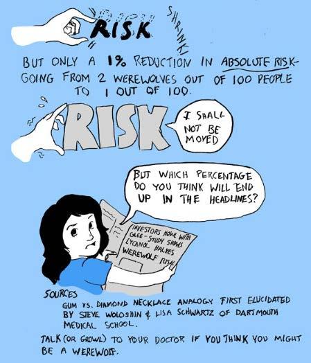
57 / /relative-riskabsolute-comic-health-medicalreporting.htm

58 Alcohol Use and Breast Cancer Appropriately interpreted as a 51% increase in breast cancer risk comparing 0 daily intake to 2+ drinks/day, translating to a 1.3% increase in the incidence of breast cancer over 10 years while the increased risk found in this study is real, it is quite small. Women will need to weigh this slight increase in breast cancer risk with the beneficial effects alcohol is known to have on heart heath, said Dr. Wendy Chen, of Brigham and Women's Hospital in Boston. Any woman's decision will likely factor in her risk of either disease, Chen said. MSNBC