Backup Strategy for Failures in Robotic U-Shaped Assembly Line Systems

Transcription

1 University of Rhode Island Open Access Master's Theses 2016 Backup Strategy for Failures in Robotic U-Shaped Assembly Line Systems Alexander Gebel University of Rhode Island, Follow this and additional works at: Terms of Use All rights reserved under copyright. Recommended Citation Gebel, Alexander, "Backup Strategy for Failures in Robotic U-Shaped Assembly Line Systems" (2016). Open Access Master's Theses. Paper This Thesis is brought to you for free and open access by It has been accepted for inclusion in Open Access Master's Theses by an authorized administrator of For more information, please contact

2 BACKUP STRATEGY FOR FAILURES IN ROBOTIC U-SHAPED ASSEMBLY LINE SYSTEMS BY ALEXANDER GEBEL A THESIS SUBMITTED IN PARTIAL FULFILLMENT OF THE REQUIREMENTS FOR THE DEGREE OF MASTER OF SCIENCE IN SYSTEMS ENGINEERING UNIVERSITY OF RHODE ISLAND 2016

3 MASTER OF SCIENCE THESIS OF ALEXANDER GEBEL APPROVED: Thesis Committee: Major Professor Manbir Sodhi Gretchen A. Macht Lutz Hamel Nasser H. Zawia DEAN OF THE GRADUATE SCHOOL UNIVERSITY OF RHODE ISLAND 2016

4 ABSTRACT The application of robotic U-shaped line layouts is becoming more important for manufacturing companies. Compared to straight assembly line layouts, U-shaped assembly lines result in cost savings, easier material handling and higher production rates. The reason for this is that U-shaped lines improve visibility and skill sharing between operators, increase production quality, reduce work in process inventory and facilitate problem-solving of appearing production failures which is shown in several researches. Key companies such as Toyota and Boeing are using U-shaped assembly lines to benefit from the advantages of U-shaped line layouts. However, few breakdown strategies are designed especially for U-shaped lines even though machine breakdowns are common. Breakdowns reduce the throughput rate and product quality and therefore strategies are needed which can ensure the targeted throughput and product quality of companies during breakdowns. In this thesis a breakdown strategy IS designed for a robotic U-shaped line which uses versatile backup robots on backup stations to cover the failures of workstation robots. Versatile backup robots are only considered in one prior study for a straight line layout and, in that study, the backup robots demonstrated a better performance than other breakdown strategies used for straight lines. The concept of backup stations with versatile robots is adapted to the robotic U-shaped line layout to identify whether backup robots can be an efficient breakdown strategy for robotic U-shaped lines. This adaptation is the placement of the backup stations between the arms of the U-shaped line layout. An automotive body shop assembly line configuration is selected for the U-shaped line layout. Ten workstations are used in the line configuration. Four positions exist for the placement of backup stations. Each

5 combination of workstations and placement positions have been analyzed to find the most efficient backup strategy for line configuration designed. The analysis starts with the one backup station, then considers two backup stations and finally three backup stations on the four possible placement options. The best option of the one, two and three backup stations are compared with four backup stations and the current breakdown strategies which are the usage of manual repair stations only and the workload reallocation of broken robots by working robots downstream the line. The criteria for the performance comparison are the cycle time and product quality which are generated for a 5%, 10% and 15%-line breakdown. For the generation of the criteria, a genetic algorithm is used which is modified from a straight line layout to the robotic U-shaped line backup strategy and current breakdown strategies. The analyses of the best placement options for the one, two, three and four backup stations options identify that the three and four backup stations options have the best cycle time and product quality for breakdowns, because they cover each workstation without the use of manual repair stations. It is shown that the three backup stations option is the best choice for the designed automotive body shop assembly line configuration. The three backup stations option has the same cycle time and product quality as the four backup stations option, but it uses one less backup station. Furthermore, the robotic U-shaped line backup strategy using three backup stations has a much better performance than the current breakdown strategies. Its cycle time for breakdowns is half as much as the cycle time of the current breakdown strategies and the robotic U-shaped line backup strategy does not use manual repair stations that generate a high product quality consciously. Due to these facts, the robotic U-shaped line backup strategy is an efficient breakdown strategy for

6 the robotic U-shaped line, because it ensures production with a smooth line flow, a continuously high product quality and the avoidance of work in process inventories for breakdowns. Nevertheless, the robotic U-shaped line backup strategy has three major disadvantages. The first disadvantage is that the backup robots have to be maintained after each operating period to ensure that they do not break down. The next disadvantage is the requirements of an intelligent conveyor system so that the backup station can be accessed without disrupting the material flow when a breakdown occurs. The last disadvantage is that the backup robots have to been equipped with several possibly costly tools, to cover the workstation robots. The final decision on which backup strategy to use is therefore conditional on the cost of equipment, but this study can easily be extended to include these factors when the data is available.

7 ACKNOWLEDGMENTS First of all, I would like to thank my advisor Dr. Manbir Sodhi for his valuable support, comments, and suggestions. His advises motivated me to face this challenging research field, acquire new skills and increase my knowledge. I would like to thank Arash Nasrolahi Shirazi for the assistance to learn the programming language Python, the offering of your genetic algorithm, and the hours of discussions to improve my research project. Thank you to my committee members Dr. Grechten A. Macht, Dr. Lutz Hamel and Dr. David Freeman for reviewing my thesis and sharing your knowledge. Additionally, I would like to thank everybody involved in the exchange program between The University of Rhode Island and Technical University of Braunschweig. Your involvement gave me the chance to be a student at URI, make new friends all over the world, and have a wonderful time in the United States of America. Finally, I would like to thank my parents Viktor and Tamara Gebel as well as my siblings Andrej and Sergej Gebel. Your support made this awesome year in the USA possible. Thank you so much and it is an honor to be a part of such an extraordinary family.. v

8 TABLE OF CONTENTS ABSTRACT... ii ACKNOWLEDGMENTS... v TABLE OF CONTENTS... vi LIST OF TABLES... viii LIST OF GRAPHS... ix LIST OF FIGURES... x CHAPTER INTRODUCTION Current Situation and Problem Statement Objectives and Approach... 4 CHAPTER Line Balancing Problem Industrial environments Product design and process layout selection Constraints and attributes leading to line balancing constraints Objective function Solution procedures Exact methods Heuristic procedures CHAPTER U-Shaped line layout Lean Manufacturing Functionality of a U-Shaped line Breakdown strategies vi

9 CHAPTER Robotic U-shaped line backup strategy design Breakdown strategies evaluation Backup strategy design and functionality Genetic algorithm for the backup strategy CHAPTER Robotic U-shaped line backup strategy analysis One backup station analysis Two backup stations analysis Three backup stations analysis Breakdown strategies comparison Breakdown strategies comparison using a five-time greater rework time Breakdown strategies comparison using a two-time greater rework time CHAPTER Critical view on the ru-sbs & further research CHAPTER Summary APPENDICES Appendix A: Kahan et al. approach [50] Appendix B: Müllers redundancy level approach [9] Appendix C: Modified Genetic Algorithm BIBLIOGRAPHY vii

10 LIST OF TABLES Table 2.1: Goldberg s Population Fitness Table 2.2: Goldberg's example offspring [41] Table 4.1: Task execution time matrix Table 4.2: Design of a capability matrix [50] Table 4.3: Task precedence matrix Table 4.4: Genetic algorithm replication test Table 4.5: Genetic algorithm replication test viii

11 LIST OF GRAPHS Graph 3.1: Comparison of Shirazi et al. [53] Graph 5.1: Mean cycle time for the use of one backup station Graph 5.2: Product quality analysis for the one backup station options Graph 5.3: Mean cycle time for the use of two backup stations Graph 5.4: Product quality analysis for the two backup stations options Graph 5.5: Mean cycle time for the use of three backup stations Graph 5.6: Product quality analysis for the three backup station options Graph 5.7: Mean cycle time of the breakdown strategies considered Graph 5.8: Product quality analysis for the breakdown strategies comparison Graph 5.9: Mean cycle time of the breakdown strategies using a five-time greater manual rework time Graph 5.10: Product quality analysis for the breakdown strategies comparison using a five-time greater manual rework time Graph 5.11: Mean cycle time of the breakdown strategies using a two-time greater manual rework time Graph 5.12: Product quality analysis for the breakdown strategies comparison using a two-time greater manual rework time ix

12 LIST OF FIGURES Figure 1.1: Chapters of the Master thesis... 6 Figure 2.1: Precedence graphs [5]... 9 Figure 2.2: Facility design factors [54] Figure 2.3: Process Layouts [5] Figure 2.4: Classification of ALB problems [15] Figure 2.5: Branch and Bound illustration Figure 2.6: Genetic algorithm concept [40] Figure 2.7: Crossover example [40] Figure 2.8: Mutation of a binary string [42] Figure 3.1: A simple U-Shaped line [6] Figure 3.2: Chase mode in U-Shaped lines [43] Figure 3.3: Double-Dependent U-lines [43] Figure 3.4: Multi lines in a single U-shapes layout [43] Figure 3.5: Embedded U-lines [43] Figure 3.6: Figure-eight-pattern U-line [43] Figure 3.7: Multi-U-line facility [43] Figure 3.8: Breakdown strategy with inventories [49] Figure 3.9: Balancing of uncompleted tasks [50] Figure 3.10: Rebalancing of a whole assembly line [52] Figure 3.11: Schematic of Backup stations for high capability robots [53] Figure 4.1: Self-generated robotic U-shaped line design Figure 4.2: Work position of robots from Station 1 [9] x

13 Figure 4.3: Four options for the robotic backup station placement Figure 4.4: Backup station option A covers broken robots of workstation 1 and Figure 4.5: Backup station option A covers broken robots of workstation 9 and Figure 4.6: Use of manual repair stations in the robotic U-shaped line design Figure 4.7: Framework of the modified algorithm Figure 4.8: Randomly generated parent gene Figure 4.9: Example of ten piece allocated to a specific workstation Figure 4.10: Example of 12 pieces for the one backup station option A Figure 4.11: Feasible number of tasks on each workstation Figure 4.12: Allocation of each tasks to one workstation robot Figure 4.13: Work time for each robot Figure 5.1: Final robotic U-shaped line backup strategy design xi

14 CHAPTER 1 1 INTRODUCTION 1.1 Current Situation and Problem Statement The methods of manufacturing have changed significantly over the centuries and these changes are described as Industrial Revolutions. In the 18th century, the first Industrial Revolution began with the use of powered machine tools [1]. The first Industrial Revolution resulted in a fundamental change from agricultural to industrial societies. Henry Ford pioneered the second Industrial Revolution by inventing mass production and assembly lines [1]. The third Industrial Revolution started in the nineteen-seventies with the development of automated manufacturing systems and programmable machines. In addition, manufacturing principles such as Lean Manufacturing have made the current production system more efficient by eliminating waste and continuous production process improvements [2, 1]. The National Science Foundation gives an American example of the consequences of ignoring manufacturing trends in their study [3]. In the nineteen-eighties the American market was overflowing with products coming from more efficient Japanese factories using the principles of Lean Manufacturing for an improved production process with less production waste, while the focus of American factories was to produce as many products as possible in the mass production flow lines. The elimination of waste in the production process leads 1

15 to a higher product quality and lower prices compared to the mass production flow lines. Thus the consumer preferred to buy the products from the Japanese factories [3]. The examples from the National Science Foundation about the American markets should demonstrate that manufacturing companies have to keep their eyes open for changing trends and production environments [3]. A study made by MHP A Porsche Company presents that the fourth Industrial Revolution arises, which involves the use of Smart Factories. Smart Factories are companies connected intelligently with their production environment which includes the connection of human, machines and resources with each other. The continuous growth of the internet and information technologies provides factories and their resources with more information that leads to transparency of information. Figure 1 illustrates an example from the MHP A Porsche Company study of Smart Factories connected over Computer Processing Systems with their environment which consist of Smart Logistic, Smart Buildings, Smart Products, Smart Grids and Smart Mobility [1]. Figure 1.1: Smart Factory [2] 2

16 Increasing individual customer needs, volatile global markets, scarcity of resources, ecological requirements and cost pressure are the current challenges for factories. The fourth Industrial Revolution will help to handle these challenges by providing factories more information about their environment that will help factories to react more flexibly to changes. According to the study of MHP A Porsche Company, the ability to react to demand variability which includes time and value aspects, using resources efficiently, customer oriented product design and production will be important features resulting from flexibility [1]. The study of MHP A Porsche Company is only a survey of the slowly increasing awareness of German companies about the upcoming trend of the fourth Industrial Revolution. Nevertheless, challenges such as individual customer needs, volatile global markets and cost pressure exist already and solutions have to be developed to handle these challenges [4]. Production optimization is one important step to increasing companies efficiency [4]. Production flow lines exist in many manufacturing companies and they require high investment and running cost. These costs have a significant influence on economic performance of the company and therefore the line balancing problem is important for the production optimization [5]. Robotic assembly lines are highly automated systems to produce finished goods. Although much research has been done in the broad field of the line balancing problems, only a few papers consider robot breakdowns despite the fact that breakdowns are common. Another common topic in assembly line balancing problems considers U- shaped layouts. Compared with the straight assembly line layout, U-shaped assembly lines result in reduced cost, easier material handling and higher production rates. The reason for this is that U-shaped lines improve visibility skills between operators, 3

17 increase production quality, reduce work in process inventory and facilitate problemsolving of appearing production failures which is shown in several researches [6, 7]. Companies such as Toyota and Boeing are starting to use U-shaped assembly lines to become more efficient [8]. Therefore, the objective of this thesis is to design a breakdown strategy for a robotic U-shaped assembly line which ensures an efficient line flow for breakdowns. 1.2 Objectives and Approach The objective of this thesis is to design a breakdown strategy for robotic U-shaped flow lines which ensures a production with a smooth line flow and a continuously high product quality. The approach for the breakdown strategy starts with a general description of the flow line balancing problem. Chapter 2 explains in detail the different constraints, optimization goals, and solution approaches which are essential to model and solve a flow line balancing problem. Subsequently, a brief description of U-shaped lines will follow in Chapter 3. The advantages of U-shaped assembly lines compared to straight assembly lines will be discussed. Furthermore, the requirements of U-shaped assembly lines will be shown and which breakdown strategies already exist for U-shaped assembly lines and for straight assembly lines. The reason for the consideration of breakdown strategies for the straight assembly lines is that the research field of breakdown strategies is limited. The consideration of a wider breakdown research field will ensure that an efficient breakdown strategy can be designed for the robotic U-shaped assembly line. 4

18 Chapter 4 evaluates the existing breakdown strategies and it designs a U-shaped line configuration which is an adaptation of an automotive assembly line body shop. For this line configuration is a breakdown strategy design that uses the various number of one, two, three and four robotic backup station on the four possible placement options in the robotic U-shaped line layout configured. Furthermore, the functionality of the various design options of the robotic U-shaped line backup strategy are described. Chapter 5 analyzes the various number of one, two, three and four backup station on the four possible placement options of the robotic U-shaped assembly line backup to identify the best performing option. In addition, the robotic U-shaped assembly line backup strategy is compared with current breakdown strategies based on its performance. The performance of the various design options for the robotic U-shaped line backup strategy and current breakdown strategies are investigated for 5%, 10% and 15%-line breakdown scenarios. Afterwards, a critical view on the generated robotic U-shaped backup strategy follows in Chapter 6. This critique shows some drawbacks which have to be considered to make the robotic U-shaped backup strategy a useable implementation for factories. The critique leads to further research requirements in the assembly flow line breakdown strategy field. At the end of this thesis is a summary of the chapters and the generated results. Figure 1.2 illustrates the chapters of this thesis. 5

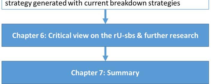
19 Figure 1.1: Chapters of the Master thesis 6

20 CHAPTER 2 2 LINE BALANCING PROBLEM The Line Balancing Problem has been widely researched. It is important for researchers as well as practitioners, because flow lines require high investment cost and can lead to high running cost [9]. Furthermore, the line balancing problem consider various restrictions and constraints, which break the line balancing down and specify it. Especially the constraints could specify the line balancing problem to current challenges of factories. An example for line balancing problem dealing with current challenges of factories is in a journal article published by Chicaet et al. [10]. It deals with the optimization of an assembly line balancing problem considering the constraints varying work time, space and uncertain demand, which are equivalences to the aspects individual customer needs and volatile global markets as current challenges of factories [10]. This chapter will review the literature relevant to the restrictions and constraints. Subsequently, the general line balancing will be zoomed in to the robotic U-shaped assembly line balancing problem. 7

21 2.1 Industrial environments The industrial environment specifies the general term line balancing problem by giving it a functionality. Common industrial environments in the academic research are machining, assembly and disassembly lines [5]. In machining lines, operations on parts such as drilling, welding, grinding and etc. are completed on several machines. Machining and assembly lines are highly automated and have to follow given precedence relations. Assembly lines produce final products and the significance is that several operations can be done simultaneously on a station with more than one machine or robots. Assembly configurations are also being investigated by disassembly line types. The research on disassembly lines is growing because of the rising governmental regulation for product recycling and therefore parts have to recycled or reused as good as possible. Nevertheless, the most disassembly lines are manual and just reversing of the precedence relations of the assembly graph gives not a working disassembly graph [5]. Figure 2.1 illustrates from the literature, an example for precedence graphs in the typical industrial environments. The circles with numbers represent a task and the arrows are the relationships between tasks. As an example, in Figure 2.1, the assembly line task 4 can just start after tasks 2 and 3 have been completed, but task 5 has just to wait for task 3 to be proceed. Companies decide their industrial environments by considering the products they are producing which leads to other two important aspects of the line balancing problem the product design and process selection. 8

22 Figure 2.1: Precedence graphs [5] 2.2 Product design and process layout selection A product design translates into a set of tasks which have to be executed to produce a specific product. Therefore, tasks are the breakdown of the full production process into logical and small steps. Following these steps leads to the required product in the defined Quality. The steps generate the precedence relationship between each other. In assembly lines a final product just could be assembled after subassemblies and components of subassemblies has been done. The technology used is also an important consideration for the precedence relationships [9]. In new facilities, the set of tasks defines the production technology that has to be purchased and the product design creates the process sequences through the whole facility. Figure 2.2 shows that the 3 factors product, process and schedule design are defining the facility design. 9

23 Figure 2.2: Facility design factors [56] Thereby the line balancing problem generates the schedule design using the defined constraints and objectives. A more detailed explanation about constraints and objectives will be given in section 2.3 and 2.4. However, when using existing production facilities, the designed product has to be completed with the existing line technology. In addition, existing production could have resulted in machines placed in a specific line layout. The line layout is crucial for the line direction and possible distribution of tasks to a special workstation. Typical line layouts are basic straight lines, straight lines with multiple workplaces, U-shaped lines and lines with a circular transfer which are shown in Figure

24 Figure 2.3: Process Layouts [5] In basic straight lines, a workpiece runs through each workstation in the given order. Thereby the required set of tasks is done one after the other and the workpiece comes from the last station as a finished good, if the industrial environment is an assembly line [7]. A single straight assembly line works for simple products. Complex products and high production intensities require a straight line layout with multiple workplaces or a U-shaped line layout for a smooth production flow. In a straight line with multiple workplaces layout several tasks can be performed simultaneously at each station. This 11

25 is essential for a smooth line flow where a specific amount of subassembly has to be done before the workpiece can enter the next station [11]. Lines with circular transfers place their workstation around a rotating table as illustrated in figure 2.3. The table is used for loading and unloading the workstations with the required material to produce the finished good. A line layout with a circular transfer can be seen as being equivalent to a line balancing problem for a basic straight line and straight line with multiple workplaces. The frequency of the turn tables decides which optimization method could be used. A single turn is equivalent to basic straight lines and multi-turn for straight line with multiple workplaces [12]. As Figure 2.3 shows, U-shaped lines have their start and end point at the same place and operator could work inside the line layout. The literature mentioned several advantages of U-shaped line layouts compared to straight line layouts [8, 13], which will be detailed further in Chapter Constraints and attributes leading to line balancing constraints Constraints construct a border for the line balancing problem in which the optimal task to workstation scheduling has to be found. Thereby constraints arise from logical, mathematical, practical conditions and from attributes of the objectives considered in the optimization [5]. A logical constraint mentioned in Section 2.1 is the precedence relationship between tasks, which have to be fulfilled to produce the required product. Another 12

26 logical constraint is the number of workstations. The line balancing optimization cannot schedule task to an eleventh workstation, if just ten workstations are given [14]. The cycle time is one of the most important constraints in the line balancing problem and it belongs to the mathematical constraints. In the literature two different definitions for the cycle time are given. The first definition describes the cycle time as the time needed to produce a finished product from the start to end of a production line in a facility. The second definition describes the cycle time as the amount of time given to each workstation to fulfill their scheduled tasks [15]. The second cycle time definition is more commonly used and the following formula shows how the upper bound of the cycle time could be calculated. / 15 The line balancing problem should consider several attribute which influence optimization [5]. Each workstation has attributes which influence the distribution of tasks to a specific workstation. These attributes could be the type and number of workers and tools assigned to a specific workstation and the buffer capacity of each workstation [5]. In the literature these types of optimization problems are described as Assembly Line Design Problems (ALDP), because they try to set up workstations optimally for the assembly tasks [16]. 13

27 Worker distribution can also be considered in the line balancing problem and they too can be defined by specific attributes. A current optimization model of Ramezanian et al. considers the different skill levels of workers and the amount of cost they cause with the scheduling to specific workstations [17]. Another important attribute mentioned in the context of the line balancing problem is that of the task attributes which could be constant, dynamic, uncertain or dependent on the assignment to a workstation. Dynamic and uncertain attributes or lead times make the line balancing problem very complex and increase the computing time required to find a feasible solution compared to that for constant and assignment dependent problems. On the other hand, dynamic and uncertain attributes reflect the practical manufacturing and even an attribute considered constant such as the task time, could become uncertain [18]. However, the optimization with constant attributes is needed to find optimal solution approximations and establish a foundation for further researches. For example, the Simple Assembly Line Balancing problem which considers constant task times, an upper bound of a given cycle time for every station and respects the precedence constraint between the tasks was introduced in 1955 and was used to minimize the number of the workstations used in a basic straight line design. Since this initial problem formulation, the related body of research has grown continuously and in just the period from 2007 to 2012, 267 scientific papers were published for this line balancing problem [5]. In practice, companies produce not just one product, but several models of a basic product and/or several different products. The literature defines the optimization problems which consider the number of products a Single-model lines, Mixed-model 14

28 lines and Multi-model lines. Single-model just considers one basic product, Mixedmodel lines consider a similar products and the Multi-model line consider different products, which are usually produced in batches [5]. It is obvious that the complexity of such problems increases significantly with the number of the products and differences between them. It is not just the number of products, that are considered in the line balancing problem. The number of flow lines is also a constraint because factories usually have more than one production line. The line balancing problem therefore includes cases with multiple lines (with identical or different configuration workstations) and workers assigned to more than one line and several parallel lines with crossover [19, 20]. Multiple lines are very complex to configure, because they must also consider constraints previously listed such as task and workstation attributes. Therefore, finding the solution becomes a time intensive and complex task [5]. However, considering every constraint mentioned above makes the line balancing problem too complex. Thus the literature has started to categorize the line balancing problem. Figure 2.4 illustrates a classification of the Assembly line balancing problem. The single model assembly line with deterministic task times in a U-shaped line layout is the simplest mentioned research field for U-shaped lines. Nevertheless, it simplifies the functionality of a production line and offers a foundation for the complex backup strategy research. Therefore, the single model assembly line with deterministic task times in a U-shaped line layout will be considered in this research. 15

29 Figure 2.4: Classification of ALB problems [15] 2.4 Objective function Another difference between line balancing problems is in the objective function. The first formulations of the assembly line balancing problem sought the minimum number of workstations to manufacture a product [21]. The types of the objective functions considered have since increased. Besides the minimization of the workstation, other objective functions are: Minimization of the cycle time. Maximization of the line efficiency. Maximization of the system utilization. Minimize the re- and configuration cost. Maximize the line profit. 16

30 The list of objective functions shows that constraints can became objective functions, because the cycle can be used as objective and constraint. The researcher defines his/her optimization goal and chooses the best fitting objective function for his purpose. Each objective function requires its own constraint variations and therefore the models in the literature vary considerably [5, 22]. Current research tries not just to optimize the production lines, but also to make them robust. In Xu et al. definition robust approaches try to find a solution or a set of solutions that performs well across all scenarios and hedges against the worst of all possible scenarios [23]. Taguchi introduced a methodology for robust optimization and defined three stages to attain robust design. The first stage is the systems design where the parameters of a product are defined in general. In the second stage these parameters are optimized to create quality requirements. These two steps are the usual steps of optimization problems which were mentioned above. The creation of a tolerance for the design parameters is the last step of this methodology [24]. Thereby tolerances are uncertainties and they could be deterministic, probabilistic and possibilistic. Deterministic tolerance gives an area in which a parameter for a task and/or workstation can vary. The second tolerance type works with probabilities in which an event change the parameters to a specific value. Possibilistic tolerances are fuzzy measures in which probabilities could appear to change parameters in to a plausible range [25]. Robust optimization increases the complexity of the line balancing problem dramatically. It considers the range of listed constraints in Section 2.3 and can consider additional parameters, while changing their values. Thus several options exist to solve robust optimization. Beyer et al. presented theoretical and practical solution options in 17

31 a survey. The theoretical methods for robust optimization such as the robust counterpart approach and the aggregation approach are not considered in the flow line balancing literature, because their complexity needs an enormous amount of computing power and time to generate a possible solution [25]. Practical methods to solve robust optimizations include evolutionary approaches such as genetic algorithms. Evolutionary approaches belong to approximate methods which do not give an optimal solution for a problem. Rather they generate a feasible solution for a problem in an acceptable computing time [5, 25]. A more detailed description about solution method will be given in the following section. Robust line balancing approaches are developed to handle uncertain data. Robust means also that the flow line should continue to operate even if one or more machines break down. Break downs are practical problems and should also be considered in robust design. Battaia et al. and Hazir et al. recommend the line balancing problem with robustness against break downs as further research [5, 26]. The literature of the assembly line balancing offers studies about break downs, because of their practical application. Therefore, in Section 3.3 the current state of the break down research will be given and especially which break down strategies could be adapted for robotic U-shaped assembly lines. 18

32 2.5 Solution procedures After considering all the parameters above, the last step in the line balancing is to choose a solution procedure to solve the problem. The solution procedures have to find the best solution for the defined constraints and objective function. In addition, the solution procedure has to execute fast. In the line balancing problem, the performance of solution procedures is measured with the required time to find an optimal solution [27]. Another important factor in the performance is the solution value. Some solution procedures provide better solutions than other procedures and therefore the literature classify the solution procedures in exact and heuristic methods Exact methods As their name suggests, exact methods find the best solution for an optimization by considering a specific number of tasks and constraints. Therefore, the objective function and the constraints have to be defined in a mathematical model. The most common model for the assembly line balancing problem is the mixed integer program. To illustrate how a mixed integer program works, the simple assembly line balancing problem (SALBP) 1 and 2 will be taken as example. These two optimization problem are very simple defined. As mentioned in section 2.3 the SALBP-1 optimizes the number of used machines by considering the constraints cycle time and precedence relationship between tasks. The SALBP-2 is similar to the SALBP-1. It uses also a limited amount of constraints, but it optimizes the cycle time for a given number of 19

33 machines. The following parameters were assumed to generate a mathematical model for the multi integer program [28, 29]: number of tasks number of workstations time to fulfill a task cycle time set of immediate predecessors of the task weight cost of an assigned workstation earliest possible workstation for task latest possible workstation for task SALBP 1 [28].,,.,,.,,, &..,.. 20

34 SALBP 2 [29]..,.,., The equation (1.1) is the mathematical formulation for the objective function of this optimization problem, which searches for the minimum number of used machines. The constraint (1.2) defines in a mathematical form, that each task could be just assigned to one machine. In the equation (1.3) is defined that the used work time of each machine has to be lower or equal to the cycle time to fulfill all the assigned tasks. In the next step the equations (1.4) defines the precedence constraint. A task can be just done on a machine if it predecessor has be done on a previous or on the same machine. The SALBP - 1 has two equations more than the SALBP 2. The equations (1.5) and (1.6) support the objective function by weighting the machines. Each time the number of machine used is increases, the new machine gets a higher weighting than the previous machine. This weighting idea should support the objective function to keep the used number of machines as small as possible. In the end is the equation (1.7) which defines the values for the variable. Thereby has the value 1 if task is assigned to the 21

35 machine and otherwise it gets the value 0. The linear definition of constraints in a mathematical model and that could just take the values 0 and 1, makes this model to a mixed integer program solution procedure. The SALBP 2 has some similar equations as the SALBP 1. The equation (2.2) defines as well that each task could be just assigned to one machine and equation (2.3) sets the cycle time as upper bound work time for each time for each machine. Thereby it has to be mentioned, that the SALBP 2 does not have a given cycle time. The interaction between the equations (2.1) and (2.3) is searching for the lowest cycle time by considering as well the other constraints. The equation (2.1) is the objective function of the SALBP-2, which is the cycle time minimization. This example should show, that an objective function can be a part of the constraints. The precedence relationship will be defined by equation (2.4), where a tasks can just be done after its predecessor. In the end the equation (2.7) makes the SALBP -2 to a mixed integer program model such as equation (1.7) does it with the SALBP 1. As mentioned in section 2.3 the line balancing problem can become very complex with the number of constraints used. Even if the set of task and machines is small, some constraints can make it impossible to construct a linearized mathematical model. In this case a nonlinear integer program could be used. A good example of this could be found by Hamta et al., who extended the SALBP-2 with flexible tasks times and a second objective function which consider the machine cost. These additional parameters made it impossible to create a linearized mathematical model and therefore a non-linear model was created to find an exact solution [30]. The linear and nonlinear integer programming model is used to create mathematical equations, which have to be solved to find the exact solution. It is practical to use special solver as Cplex, LINGO, ILOG to generate 22

36 a solution. These solvers follow the branch and bound algorithm to generate the exact solution [5]. The branch and bound algorithm can be seen as a tree diagram. It creates several levels of branches. At each level the algorithm compares the value of the branches and let just the branch grow, which has the best value. Here best means a low value if it is a minimization problem and a high value if is a maximization problem. The branch and bound algorithm creates as long level of branches as the entire of set parameters are considered in the tree diagram [31]. It is difficult to illustrate a line balancing problem in a branch and bound algorithm, because it becomes very huge even with a small set of parameters. Therefore, Figure 2.5 shows the basic idea of the branch and bound algorithm. In this example 4 task has to be ordered in an optimal position and from the start point the task 1 and 4 have the same value and a better value than task 2 and 3. Thus the branch and bound algorithm follow these branches to find the optimal solution. Figure 2.5: Branch and Bound illustration 23

37 The possibility to find an exact solution is just one aspect of evaluating the performance of solution procedures. Another criterion is the required amount of time to find the exact solution. Thus the researchers try to modify their mathematical model with task specific bounds. A current example for a modified model is the branch, bound and remember algorithm from Sewell el al. which is branch and bound approach combined with dynamin programming [32]. The branch and bound part eliminates sub problems, which cannot offer a better solution than the current found branch solution. The dynamic program remembers all calculated solution and avoid that a solution option is calculated twice solve. Thus branch, bound and remember algorithm can solve the simple line balancing problem faster than any other exact algorithm [32]. Dynamic programming is a fast method to generate an exact solution. It divides a problem in sub-problem and generates solutions for the sub-problem. Afterwards the best solution is generated out of the sub-solutions by changing the sub-problems until the best solution is found for the initial problem [33]. The literature describes line balancing as NP-hard. Thus the required solution time increases exponentially with the parameters such as task size and the number of workstation used. With more parameters and uncertain data, exact solution may not be found. Therefore, approximate procedures have been developed to solve optimization problems with a large amount of sets, uncertain data and several objective function [10, 34]. 24

38 2.5.2 Heuristic procedures Heuristic procedures may not find the optimal solution for a line balancing problem, but they find acceptably good solutions even for complex problems in an acceptable amount of time [5]. The literature categorizes approximate procedures into simple heuristic and metaheuristic methods. Simple heuristic methods use greedy algorithms or priority rules to generate a feasible solution for a large problem size in an acceptable time amount. Most priority rules are used for tasks or workstation attributes, which increase the complexity for the solution finding as mentioned in section 2.3 [35]. In addition, the user of simple heuristics methods can decide what an acceptable solution search time is. Therefore, they have to define how many iterations their method does until it stops and delivers the feasible solution. Needless to say that a low number of iterations do not usually generate near optimal solutions. Nevertheless, simple heuristic methods are often used to generate an upper bound for exact solution methods and these are used to find an optimal solution for a large problem size [35]. Metaheuristic methods are used for optimization problems with large problem sizes and complex constraints. Mostly a mathematical model cannot be created to solve such problems and metaheuristic methods are able to generate a near optimal solution. Metaheuristic methods are build up in a programming language as C, C+, Pascal or Python and follow specific algorithms. 25

39 Some of the heuristic approaches used in the literature for the solving of the line balancing are: Neighborhood methods [36] Evolutionary approaches [37] Swarm intelligence approaches [38] The neighborhood methods are used for the optimization of multi-objective problems. The optimization starts by finding the best solution for the first objective. Afterwards, the second objective is considered and the neighborhood methods searches near the area (neighborhood) of the best solution for the first objective to find the best trade off solution for both objectives [36]. The swarm intelligence approaches base on the natural behavior of animal swarms in the food search process. In the optimization problems, the objective represents the food and a several number of search function, which is defined by the user of the swarm intelligence approach, represent the individuals in a swarm. The search functions start the solution search process simultaneously over the whole search area. After the finding of a good solution that has to be defined by the user in the initial phase of the swarm intelligence approach, all research functions concentrate on the area of this good solution generated, to find a better solution for the optimization problem [37]. The evolutionary approaches are based on natural behavior as well. The complexity of these methods makes it difficult to illustrate them. Thus the genetic algorithm will be used to demonstrate the evolutionary approaches. The genetic algorithm is a part of the evolutionary approaches and the most widely used metaheuristic method [5]. John 26

40 Holland introduced the genetic algorithm for the first time in The Genetic algorithm is an abstraction of the biological evolution process adapted in a computer system [39]. Figure 2.6 illustrates how the biological evolution process adapts in an algorithm. Thereby all stages will be explained with the biological logic in them and how this logic gets translated into an algorithm. The first step of a genetic algorithm is to initialize a population. These will be the first parents of several generations that follow. In the line balancing problem this population exist of a chosen amount of possible solution for an optimization problem. All the parameters of the considered constraints are genes and their connection build up a string called chromosome [40]. In programming languages all kind of alphabets can be used to design chromosomes. A binary alphabet will be used to show how the genetic algorithm work based on example of Goldberg [41]. Nevertheless, numerical and characters can also be used as alphabets. The process to choose an alphabet and design the chromosomes is called coding in the computer language. The second stage in the genetic algorithm is to evaluate the fitness of the population. Fitness is the value which gets generated by chosen chromosomes. A high value is good or bad depends on the objective function. If the objective is to minimize the cycle time, a lower cycle time is better than a higher. Goldberg choose in his example the function f(x) = x 2 in an interval from 0 to 31 and he wanted to maximize the value of f(x). Therefore, he chooses randomly 4 numbers as population, programs them as chromosomes in a binary algorithm and evaluate their fitness as shown in Table 2.2 [41]. 27

41 Figure 2.6: Genetic algorithm concept [40] Parent No. Real No. Binary No. Fitness f(x) Table 2.1: Goldberg s Population Fitness 28

42 Constraints Satisfaction is the third stage of the genetic algorithm. In this stage it has to be proven whether all parents fulfill the defined constraints. In Goldberg s example the only constraint is that the number found should be in the interval between 0 and 31. All chosen parents in Goldberg s example are in this interval and there they all fulfill the given constraints [41]. However, the best solution for f(x) = x2 in the interval between 0 and 31 has not been found yet. Therefore, the genetic algorithm has an additional constraint. This constraint is the number of iterations, which the algorithm has to do. Iterations means how many generations of possible solution the algorithm produce until it can stop. In the given example the algorithm is in it 0 iteration, because it is first generation of solution. The following stages will show how generations of solutions are created [39]. The fourth genetic algorithm stage is select survivors. The programmers decide how many parents of the population will be used in the next stage. This shows that genetic algorithms are individual designed to solve optimization problem and a general genetic algorithm does not exist [10, 39]. Nevertheless, it is logical to use the parents with the best fitness. Goldberg use 4 parents in his example. Therefore, he chose the best 3 parents to randomly vary individuals [41]. Randomly varying individuals is the next stage of the genetic algorithm. This is the reproduction stage in where the children of the survival population are made. Two methods exist to produce the next generation. These methods are crossover and mutation [40]. Crossover means that two parents generate two offerings. Each offspring has the genes of the two parents. The programmer of the genetic algorithm decides how many 29

43 genes of a parent go to an offspring. Thereby, the parent chromosome can be cut down in a chosen number of genes and distributed to the two offspring. Figure 2.7 shows a crossover with one cutting point. Figure 2.7: Crossover example [40] Mutations modify one or more genes in the created offspring. As in nature the mutation probability should be low in the genetic algorithm [40]. In the end the programmer has to decide which mutation probability is used or if the genetic algorithm should use only crossover to search for the best solution. Eiben et al. recommend to use mutation to find better solutions [42]. The crossover search consists only of solutions, which are combined of the two parents. Using mutation brings new information in the solution area and can identify much better solution, because the first parent generation is generated randomly. In Figure 2.8 is the mutation of a binary string shown. Figure 2.8: Mutation of a binary string [42] 30

44 Goldberg s example use just crossover to create the first offspring generation, because the probability for mutation in the first iteration is very low. In addition, he uses the best three parents as survivors. As mentioned above two parents create two offspring. Therefore, Goldberg uses the best solution twice to create four offspring [41]. Table 2.3 illustrates Goldberg s first generation of offspring. Parent Offspring String Value Fitness String Value Fitness Table 2.2: Goldberg's example offspring [41] The stage randomly varies individuals ends with the creation of the offspring and leads the algorithm to evaluate fitness and afterwards to the constraint satisfaction stage again, which work the same as illustrated above. In this stages the offspring created become the new parents and the stages will repeat until the defined amount of iterations has been completed. If this happens, the algorithm will go to the last stage to output results. In the last stage the current offspring is taken and the offspring with the best fitness is presented as the best solution for the problem. As mentioned above approximate solution procedures may not deliver the best possible solution but a near 31

45 optimal solution. In Goldberg s example a near optimal solution could be found even after first iteration (see Table 2.3). The detailed explanation of the genetic algorithm should underline the key factors, which make the genetic algorithm to most used method for complex optimization methods: Solution search start from a population and not just from a single point Parent population can be generated randomly Using probabilities for creating offspring (mutation and cut points) User creates coding part individually to design the chromosome and to validate their fitness [41] These criteria make the genetic algorithm to flexible optimization method which can be used for a large amount of optimization problems, because the user created coding part can be adapted to numerous optimization problems. The random research starting points offers the chance to find good solution in several solution areas, which allows to solve complex problems. Furthermore, the more iteration the genetic algorithm does, the merrier the response will be as shown in table 2.3. Thus the user can get a good solution even for a self-defined number of iterations. 32

46 CHAPTER 3 3 U-SHAPED LINE LAYOUT Japanese factories started the use of U-shaped production layout to build up a justin-time (JIT) production. Miltenburg underlies in his survey of U-shaped production lines, that some writers see the U-shaped line design as the most effective technique for a just-in-time production [43], which will be shown in this chapter. JIT belongs to the Lean Management principles. Therefore, the following chapter will give a short overview of Lean Management. Afterwards the idea and the advantages of U-shaped production lines will be presented. In the end of Chapter 3 an overview of breakdown strategies for assembly line will be given and shown which breakdown strategies are especially used for U-shaped production lines. 3.1 Lean Manufacturing Lean Manufacturing based on the Toyota Production System, which development started in 1959 by Dr. Shigeo [44]. It is a continuous improvement in the production process to satisfy the customer requirements in terms of cost, quality and delivery times by reducing lead time, cost, improving the process flow and on the elimination of waste generated in the production environment and all activities that do not add value to the enterprise [45, 46]. Toyota proofed, that the principles of Lean Manufacturing are 33

47 successful and today Toyota is a benchmark for other manufacturing companies. The identification and elimination of seven types of wastes is one of the basic principles of Lean Manufacturing. The first type of waste is the waste from producing defects. The later a defective product is detected, the more this defect will cost. A defect product identified by a customer has to be repaired or replaced and can lead to the loss of customer. But even if defects are detected as soon as possible, they lead to cost in detecting and repairing them. In the worst case the unfinished good has to be thrown away and this leads to additional cost, which the customers are not willing to pay. Therefore, the production process should be done right and every step of the productions should be defined in the product design phase correctly [47]. Another type of waste is the waste in transportation. Material has to move through different stations until it becomes a finished good. Thus the layout of the facilities and the routing sequence of operations should be optimized to deliver the minimum transportation cost as possible [47]. The third waste is the waste from inventory. "Toyota calls inventory the roof of all evil" [47]. Every item, which sits in the inventory, causes cost and binds money that could be invested in other opportunities. Moreover, inventory hides the company problems as inadequate market intelligence, instability and worse quality of the production process. To perform a better productions process, inventory should be eliminated [47]. Waste from overproduction belongs also to the seven wastes of lean manufacturing. The production output of companies is much higher than the customers demand for a 34

48 product, which leads to inventories. Companies do this to keep their workers and machines busy and get low unit prices. But unsold units produce also cost, which has to be carried by the sold units. In the end each over production unit just leads to more cost. Furthermore, if everyone has to be busy, no one gets the chance see the emerging problems of the company [47]. The next waste in Lean Manufacturing is the waste of waiting time. This waste includes waiting for orders, parts, materials, items from preceding processes, or for equipment repairs [47]. It is a sign for a flawed process flow, if waiting appears. Moreover, waiting time increases the unit cost, for which the customer has to pay, and in addition the customer has to wait longer [48]. Another waste is the waste in processing. Every task, which doesn t add value to a product, should be eliminated. Additionally, each process should be improved, if the improvement makes the process more efficient [47]. The last waste of lean manufacturing is the waste of motion. This waste takes a deeper look on every step of a process and tries to eliminate each unnecessary movement to make the process much more efficient [48]. Eliminating the seven wastes of Lean Manufacturing results in an efficient production process with a high quality. For achieving this a Total Quality Management System is needed, which is also an important part of Lean Manufacturing. The term Quality is defined it from the interaction of the customers and producer s perspective. Customers buy products to fulfill their needs, which have to be translated by the producers to the basic quality of their products. This translation occurs in form of the product design and manufacturing. By including the other departments as 35

49 engineering, manufacturing, marketing, sales and the suppliers the Total Quality Management gets defined. Thus everybody shares an idea of how their performance should be. The workers start to proof the work in process and give a feedback to their predecessor, because a failure performance of the predecessor cannot be recovered by the current station. In addition, everybody has to be watchful and flexible, because the needs of the customers are changing continuously and therefore the companies have to change and improve their understanding of quality continuously. The elimination of the seven wastes and Total Quality Management stipulates, that only goods should be produced, which fulfill the quality and the demand of the customers. Hence it is logical, that Lean Manufacturing includes a process of controlling production and this starts with the customer [47]. Pull Production is the term for this method and it was developed in the 1950s by Toyota. American supermarkets first implemented these methods and they were adopted to the manufacturing industry. Each time a customer buys a product, the predecessor station is allowed to send an order to their predecessor station [48]. This procedure should ascertain, that only needed goods are produced and it deviates from the old form of Push Production. Push Production is the opposite production method, which try to produce as much goods as possible. The idea behind Push Production is to get low unit cost. Discounts should secure, that customers are buying this huge amount of products [48]. It is difficult to state in general terms whether pull or push production is better, because it depends on the products. If a product is standardized such as toothpicks, push production is better to get low unit cost and a huge volume of products. But if a products 36

50 get more specific, then the pull production is better suited to fulfill the needs of the customers [47]. To realize the concept of pull production, the two aspect of Lean Manufacturing needed are Just in Time and SMED. Just in Time is a concept with the main idea being that a station gets its required material in the needed moment and in the right amount. This concept supports the idea of the elimination of inventory. To fulfill the requirements of Just in Time, the delivery of the material has to be optimized and the delivered material has to fulfill the standards of Total Quality Management [48]. SMED means Single Minute Exchange of Die. This concept is more a methodology developed by Shingo [47], which has the goal to reduce the time, where a machine or an operation has to been stopped to change a tool, to a single minute. In the practice a minute to exchange a tool could not be realized for a long time [47]. Today, automotive assembly line robots use more than one welding gun for their tasks execution and could change the welding guns used in a few seconds [9]. Lean manufacturing follows the concept of a continuous improvement, also called Kaizen, which makes it to a dynamic production strategy. Continues improvement means that mistakes are analyzed in-depth to find and solve the reason for the mistake, learn from it and never repeat the mistake again. The concept of Kaizen also extends to the workers. They should get the chance to improve and raise their knowledge and skills through different projects and task to become an important part of the company. 37

51 3.2 Functionality of a U-Shaped line In a U-Shaped production line are the producing machines arranged in a U form. Thereby the start and the end of the production line are at the same vicinity. Operators work inside the U-Shaped line design as illustrated in the following Figure [6]. It is possible to place the operators outside the line, if the machines allow an operation from both sides. Nevertheless, the literature places the operators in the middle of lines and this concept will be used in the following. Figure 3.1: A simple U-Shaped line [6] The movement of the Operator and the production flow can be clockwise or counterclockwise [6]. The flow direction can be decided by the line balancing decision and which balancing direction delivers the best line efficiency. In Miltenberg s description of the U-shaped line, no further material is allowed to enter the line while a product is still in work [43]. Thus the idea of Just-in-Time should be fulfilled to produce 38

52 just a product then it is needed. Additionally, it become easier to stop the machines if a problem with a product or machine appears. This production flexibility should be able to generate the required quality with zero product defects. Miltenberg defined, in his survey of U-shaped production lines, the chase mode. Originally the chase mode means that one operator works at a U-shaped line and convoys the products through all the workstations. More common is that two or three operators run a U-shaped line. In this scenario the operators are assigned to a specific section of the line and fulfill their scheduled tasks for each product. Figure 3.2 shows the chase mode with one operator and two operators. Figure 3.2: Chase mode in U-Shaped lines [43] 39

53 One operator is able to run a whole production line, because there is a separation of work by the operator and the machine work. The operators work usually consists of: 1. bring the work in process part to the required machine 2. load the machine with the part and other requirements 3. start the machining process 4. wait a short to check if everything is alright 5. unload the work in process part 6. check the quality of the part [43] The machine work is the automated part work with the machining functions as drilling, welding, assembly or other machining process which are needed to produce a product in the required quality [43]. One big advantage of U-shaped lines over straight lines is the better rebalancing possibilities. Rebalancing includes the following three functions: varying the production rate moving machines changing standard operations [43] Varying the production rate means including operates to increase the production rate or removing operators to decrease it. Flexible and multi-skilled workers are needed to adapt the current production rate to the required demand. This leads to better educated workers and make the production job more interesting [43]. 40

54 Moving machines and changing standard operation are necessary for new products and technological production innovation. As mentioned in section 2.2 the product design and production technology are the decisive part for the production tasks. With innovations, new tasks appear which requires additional precedence relationship and other machines. Therefore, moving machines and changing standard operations is essential for a smooth production and flexible production rates [43]. The current description of U-shaped production lines refers on the simple U-shaped line design. In Section 2.3 it was mentioned how complex the line balancing problem can become with multi-lines. In practice it is common to have more than one simple line. The following figures illustrate how other configurations of more complex U- shaped lines are discussed in the literature. Figure 3.3: Double-Dependent U-lines [43] 41

55 Figure 3.4: Multi lines in a single U-shapes layout [43] Figure 3.5: Embedded U-lines [43] 42

56 Figure 3.6: Figure-eight-pattern U-line [43] Figure 3.7: Multi-U-line facility [43] 43

57 All the U-shaped lines above are designed for a practical use with multi-product production. It is not common and too laborious to reorganize the whole production line for product changes. In addition, each layout can vary their production rate by adding workers to the lines. Figure 3.7 is the most complex layout design, because it structures the whole facility in a U-shaped layout [43]. These complex U-shaped line designs illustrate the advantages of U-shaped lines. The first advantage of the U-shaped layout is the increased visibility and communication in the production process. Thus the production quality increases and problems are solved much faster, because workers recognize problems faster and can help each other to solve it [6]. Another advantage is that workers become much more skilled. Workers are scheduled between workstations and different lines to vary the production rate. This work rotation makes the work more interesting and the workers learn many more tasks, which also helps them to react more efficiently to emerging problems [6]. The next advantage is the possibility of the line rebalancing. The flexible reaction to demand helps companies to fulfill the requirements of lean manufacturing to avoid inventory, overproduction and to increase the production quality [6]. The last advantage is that U-shaped lines requires fewer workstations than straight lines, because they offer more possibilities to schedule tasks. This leads to less investments for U-shaped lines and a higher production quality can be reached with less invested money [6]. 44

58 3.3 Breakdown strategies Battaia et al. and Hazir et al. refer in their surveys about the line balancing problems to considered machine breakdowns in further research [5, 22]. The research on breakdown strategies is limited and can be categorized in the following options: Inventories Balancing of uncompleted tasks Rebalancing of the whole line Backup robots All of the breakdown strategies mentioned are mainly used for straight assembly lines. Only the inventory breakdown strategy was used for the U-Shaped line layout. Miltenburg compared the effectiveness of U-shaped lines with straight lines for machine breakdowns, which will be explained in the following [49]. Figure 3.8: Breakdown strategy with inventories [49] 45

59 Figures 3.8 shows Miltenburg s experiment design. It is simple designed with three workstations, seven tasks and a manageable amount of precedence relationships. Despite all their advantages are U-shaped lines are more efficient than straight lines, if inventories of work in process parts are placed after every workstation. If the placement of inventories after a workstation is not possible, a straight line layout should be used for proper high volume production even during breakdowns [49]. Another breakdown strategy is the balancing of uncompleted tasks. If a machine breakdown appears, the scheduled tasks of the broken machine cannot be performed. Kahan et al. introduced a mixed integer program formulation for the rebalancing of tasks from broken machines [50]. Appendix A includes the mixed integer formulation of Kahan et al. They used the design of an automotive body shop, where a car body runs through workstations and welding robots add parts until it is completed. Each station has several robots, which can perform several task simultaneous [50]. The following figure illustrates the experiment design of Kahan et al. Figure 3.9: Balancing of uncompleted tasks [50] 46

60 In addition to the mixed integer formulation, Kahan et al. tested what the best distribution for the uncompleted task is. In their test the objective function is to minimize the cycle with the reallocation of the uncompleted tasks to working stations. The response of this test is very clear. Manual repair stations had the worst performance with the highest cycle time. On manual repair stations, workers do to all the required work manually to complete the tasks of the broken machine. The best performance has the breakdown strategy with the reallocation of uncompleted tasks to working stations downstream the flow line [50]. The reallocation of tasks from a broken to a working workstation is possible if the working workstation has the same equipment or capabilities as the broken one. Additionally, the precedence relationships between tasks have to be respected. The redundancy level maximization of assembly line with a specific number of tools at workstations is a possible way to resolve breakdowns. Furthermore, tool redundancy simplifies task reallocation. Müller formulated a mixed integer program with the objective function of tool redundancy to handle robotic breakdowns in assembly lines [9]. Müllers optimization model consists of two steps. The first step finds the minimum cycle time for the user researched assembly line balancing problem. Afterwards, the found cycle time is taken as an upper bound work time for all workstations and a second optimization tries to find the best redundancy level, which should ensure the line performance for breakdowns. Müllers mixed integer optimization model can be seen in appendix B [9]. 47

61 Shin et al. created a decision tool for uncompleted task reallocation. This decision tool has been designed as a practical approach based on variables as repair time and inventory size. The objective of the tool is to decide if the uncompleted part should be allocated to a working station or a manual station to secure the required throughput [51]. The third breakdown strategy is the Rebalancing of the whole line without the consideration of the broken workstation. While Kahan et el. just wanted to reallocate the task of the broken station to deliver a fast possibility of task reallocation, other authors have balanced all task to the working stations. A current research of Sanci presents a branch and bound algorithm, which balance all tasks in a feasible way after a breakdown [52]. The objective function is to minimize the cycle time to secure a smooth production flow even with fewer working machines. Figure 3.10 shows the basic idea of Sanci s branch and bound algorithm. Figure 3.10: Rebalancing of a whole assembly line [52] 48

62 Sanci s branch and bound algorithm is the Rebalancing of a whole flow line, but just with fewer workstations. The goal is to make balancing algorithm faster and to increase their reaction time on breakdowns. In addition, the Rebalancing of all tasks requires a tool redundancy at all stations, which is similar to the breakdown strategy balancing of uncompleted tasks. The last breakdown strategy is the use of backup robots, which was introduced by Shirazi et al. and realized in a multi-objective genetic algorithm [53]. This algorithm starts with a regular line optimization by scheduling tasks to the given number of workstation under the objective of a cycle time minimization. The special feature in this algorithm is the availability of additional backup stations for workstation with a high capability [53]. Stations with a high capability have a higher probability to break down than stations with an average and low capability. Therefore, just high capability stations need a backup station to avoid breakdowns. Shirazi et al. [53] tested his algorithm in the scenario of an automotive body shop assembly line, which is illustrated in the following Figure Figure 3.11: Schematic of Backup stations for high capability robots [53] 49

63 The backup stations support the high capability stations in a normal situation without a breakdown by taking some tasks away from the high capability stations. In Figure 3.11 workstation robots R1 and R4 have a high capability and hence they get supported by the backup stations 1 robots. Then a robot breaks down, the backup station just performs the tasks of the broken robot to keep a smooth production flow [53]. The objective of the multi-objective genetic algorithm of Shirazi et al. was to create a solution method, which does not require a high tool redundancy. A high tool redundancy leads to high investment cost and an inefficient production layout. Therefore, Shirazi et al. compared their solution method with other tool redundant solution methods [53]. The following graph illustrates the comparison between the multi-objective genetic algorithm of Shirazi et al. and the tool redundancy methods. Graph 3.1: Comparison of Shirazi et al. [53] 50

64 Graph 3.1 uses the criteria cycle time and group of tasks performed on manual repair station. The lower the cycle time is the better is the performance, because a low cycle time ensure a high production throughput. Furthermore, robots offer a higher product quality than manual repair stations and therefore the fewer tasks are executed on manual repair stations, the higher is the product quality [53]. Graph 3.1 shows that the breakdown strategy with backup stations have nearly the same performance as a tool redundancy breakdown strategy with a six level redundancy. A Redundancy level is the average number of robots, which can perform one task [9]. The backup station solution of Shirazi et al. has also a 2.5 level of redundancy [53]. A six level redundancy requires much more investment than just a 2.5 level of redundancy, because the cost for tools can become very high. Nevertheless, both solutions need manual stations for breakdowns. In the method of Shirazi et al. the user has to decide what a high capability for workstations is and where a backup station has to be placed. If the capability on some workstations is not high, the user will not place a backup station there. In this case are manual stations needed for the low capability stations to secure a continuous production flow for a robot breakdown [53]. 51

65 CHAPTER 4 4 ROBOTIC U-SHAPED LINE BACKUP STRATEGY DESIGN The previous Chapters gave a detailed explanation of the line balancing problem and U-shaped line layout. The goal of this Chapter is to design a backup strategy for the robotic U-shaped line, which is efficient and fulfills the requirements of lean manufacturing. Therefore, the breakdown strategies mentioned in Section 3.3 will be validated for their adaption ability to robotic U-shaped line. Afterwards, the functionality of the backup strategy designed will be explained. At the end of this chapter will be an explanation of the methodology to investigate the performance of the robotic U-shaped line backup strategy designed. 4.1 Breakdown strategies evaluation Section 3.3 presented the breakdown strategies for the line balancing problem. The U-shaped line layout was designed as an effective technique for a just-in-time production as a part of the lean manufacturing principles. Only Miltenburg s inventory breakdown strategy is especially designed for U-shaped production lines, because the research field for breakdown strategies is very limited and the most breakdown strategies are designed for straight lines. At this point appears a discrepancy between the inventory breakdown strategy and the lean manufacturing principles of waste 52

66 elimination in form of inventories. This discrepancy has to be considered in the generation of an efficient breakdown strategy which supports the basic idea of U-shaped lines to improve the production with lean manufacturing. The breakdown strategies balancing of uncompleted tasks and rebalancing of the whole line are mainly used for straight production lines. These breakdown strategies fulfill the principles of lean manufacturing much better than the inventory breakdown strategy, because they generate a smooth line flow without additional inventories. Thus it could be an opportunity to transfer one of these breakdown strategies for the U-shaped line layout. However, it has to be accepted that the balancing of uncompleted tasks and rebalancing of the whole line breakdown strategies need a tool redundancy on the used workstations. This fact is as well a discrepancy with the lean manufacturing principles mentioned in Section 3.1. Tool redundancy is a waste in processing, because during normal production conditions without breakdowns, the workstations are equipped with much more tools than needed. This leads to higher investment cost and binds money in the production lines which could be used more efficient in other departments. Furthermore, the working workstations take the workload of the broken ones. Thus the workload increases of the working workstations. A higher workload claims the workstations for larger durations and the probability of a breakdown increases. Consequently, these breakdown strategies make the production line more unstable during breakdowns. Due to this fact, the balancing of uncompleted tasks and rebalancing of the whole line breakdown strategies belong not to the best options for a U-shaped line backup strategy. 53

67 The breakdown strategy of Shirazi et al. is designed for straight lines and uses versatile backup robots. The use of backup robots has two major advantages. The first advantage is the backup robots support of workstations with an above average workload for a normal production without breakdowns. Thus breakdowns can be avoided with the reduction of high workloads. Furthermore, the cycle time can be reduced which increases the production throughput. During breakdowns the backup robots only focus on the tasks of the broken robots. This leads to a small increase of the cycle time and a high throughput can be still reached. Additionally, other workstations will not be influenced by a breakdown [53]. These advantages make the breakdown strategy of Shirazi et al. the best of the options considered and thus it offers the potential for an adaption to the U-shaped line layout. Nevertheless, the breakdown strategy of Shirazi et al. has some disadvantages. The user has to decide what a high capability for the used workstations is and how many robotic backup workstations the algorithm should use. Additionally, manual repair stations are needed for workstation which do not get a robotic backup station. Manual repair stations have two great disadvantages compared with robotic backup stations: a work time which is up to three times greater as reported in Kahan s et al. research [50] a lower product quality. 54

68 These disadvantages affect the line performance dramatically, because the cycle time gets much higher and the product quality decreases. Due to these facts, the U- shaped line requires a breakdown strategy which can avoid manual repair stations, has an efficient number of backup stations and can handle breakdowns with an adequate cycle time increase. A robotic U-shaped line has the ability to provide these factors for an efficient breakdown strategy. In Section 3.2, it was noted that the place between the top and the bottom part of the U-shaped line is used by operators. A robotic U-shaped line works automatically and does not need operator to perform on the workstations [8]. Thus, robotic U-shaped lines have unused space between their arms. The following Section will demonstrate how the unused space could be used to generate an efficient breakdown strategy. 4.2 Backup strategy design and functionality An average U-shaped line consist of ten workstations [43]. This thesis will use the average number of ten workstations to design a practical breakdown strategy. The first step for the breakdown strategy design is to illustrate the placement and the design of the chosen number of ten workstations in a robotic U-shaped line. Figure 4.1 shows the self-generated robotic U-shaped line layout which is used for a breakdown strategy design. 55

69 Figure 4.1: Self-generated robotic U-shaped line design The self-generated robotic U-shaped line design is an adaption of an automotive body shop assembly line, which is also used by Shirazi et al. to test the performance of their breakdown strategy [53]. An automotive body shop assembly line has four robots on each workstation. Each robot has a number of tasks which have to be performed on a specific position of the car body. As example, workstation 1 will be taken from the self-generated robotic U-shaped line design to demonstrate the performance of each workstation robot. The robot with the number 1 performs the tasks on the left and rear position of the car body. Robot 2 performs the tasks on the right and rear position and robot 3 perform the tasks on the front and left position. The last robot with the number 4 perform the tasks on the front and right position. The following figure summarizes the description of workstation 1. 56

70 R1 Left R3 Front Rear R2 Right R4 Figure 4.2: Work position of robots from Station 1 [9] Figure 4.2 shows that each robot on a workstation concentrates on a specific side and position of the car body. Thus robots can break down on a workstation and the other robots on the same workstation are still able to execute their tasks. This leads to the assumption that the precedence relationship between tasks constraint exist not between robots on the same workstation. The precedence relationship between tasks constraint has to be only considered within a robot and between workstations. This assumption offers the opportunity to design a breakdown strategy with an efficient number of backup stations. The reason for this is that the robotic U-shaped line offers four options for a backup station placement and the usage of all options allows the coverage of the whole robotic U-shaped line. Figure 4.3 illustrates the four options for the robotic backup stations placement. 57

71 Figure 4.3: Four options for the robotic backup station placement Each backup station consists of two backup robots. The placement of backup stations between the arms of the U-shaped line allows the coverage of four workstations by one backup station: Option A covers workstation 1,2,9 and 10 Option B covers workstation 2,3,8 and 9 Option C covers workstation 3,4,7 and 8 Option D covers workstation 4,5,6 and 7 The backup station option A will be used as example to demonstrate how one backup station is able to cover four workstations. Figure 4.4 and 4.5 illustrates the coverage of four broken workstation robots by backup station option A. 58

72 Figure 4.4: Backup station option A covers broken robots of workstation 1 and 2 Figure 4.5: Backup station option A covers broken robots of workstation 9 and 10 59

73 In the Figure 4. and 4.5 the robots 1 and 4 on the workstation 1, robot 3 on workstation 9 and robot 2 on workstation 10 are broken. All these workstation robots are covered by the backup robots on backup station option A. Thereby, the car body enters the backup station twice. The first entry is after workstation 1 where backup robot 1 is covering workstation robot 1 and backup robot 2 is covering workstation robot 2. The next entry of backup station option A is after workstation 9. In the process backup robot 1 covers robot 3 of workstation 9 and backup robot 2 covers robot 2 of workstation 10. The coverage of two different workstations with only one backup station entry is possible, because of the precedence relationship between tasks constraint mentioned above. This constraint assumes that the tasks precedence relationship consists within a robot and between workstations. Thus backup station option A can cover the broken robot from workstation 9 and additionally it can execute the tasks from the broken robot of the following workstation 10. In this scenario backup station 1 has an above average workload, because each backup robot covers two workstation robots. Therefore, the cycle time of this backup station is the sum of the first and second entrance. The usage of all robotic backup station options allows the coverage of the whole U-shaped line. Thus manual stations are not needed, which leads to a constant high product quality. Furthermore, operators do not have to wait on manual repair stations until a breakdown occurs. Rather operators can concentrate on the line performance and react much faster on breakdowns to repair the broken robots. The operator can enter the inner of the U-shaped line configuration while the workstations execute tasks. The conveyor systems of automotive body shop uses overhead conveyors which means that the flow line can be crossed while the workstations execute tasks [54]. Consequently, 60

74 the robotic U-shaped line backup strategy designed with four robotic backup stations fulfill the requirements mentioned above of an efficient backup strategy which avoid manual repair stations, use an efficient number of backup stations and handle breakdowns with an adequate cycle time increase. Nevertheless, the question appears whether four robotic backup stations are really necessary to design a breakdown strategy with a good performance. Industrial robots are expensive and the usage of more backup robots than needed would be a waste in processing which is against the principles of lean manufacturing. Hence, this thesis will test all the possible options of backup stations placements to find the best backup strategy for the robotic U-shaped line. The possible options of the backup stations placements are: One backup station on the places A, B, C or D Two backup stations on the places AB, AC, AD, BC, BD or CD Three backup stations on the places ABC, ABD, ACD or BCD Four backup stations on the places ABCD The usage of only one backup station do not allow to cover each workstation. Due to this fact the backup station options, which are not able to cover each workstation, get a manual repair station. Figure 4.6 uses the one backup station option A to demonstrate the use of manual repair stations. 61

75 Figure 4.6: Use of manual repair stations in the robotic U-shaped line design In this scenario robot 1 on workstation 3 and robot 2 on workstation 4 are broken. Furthermore, the backup station option A is used which can cover the workstation 1,2,9 and 10. The broken robots are out of the reach of the used backup station. Due to this fact the broken robots have to be covered by manual repair stations. The manual repair stations are placed at the end of each workstation which is an adaption of the manual repair station use of Kahan et al. [50]. For a realistic comparison between the backup station options, the manual repair station usage has been extended. In Kahan et al. design the manual repair stations cover only the broken robots of the previous workstation. The robotic U-shaped line design has the assumption that the precedence relationship between tasks constraint has to be only considered within a robot and between workstations. Thus the manual repair station 3 in Figure 4.6 is able to cover the failure robots of workstation 3 and 4. Furthermore, manual repair station 4 is also place in Figure 4.6 to cover the failure robots of workstation 4. The placement of a manual repair station after each workstation should support an acceptable line performance, although 62

76 their performance is much worse compared to robotic backup stations. The disadvantages of manual repair stations compared with robotic backup stations is mentioned in the previous section. Nevertheless, manual repair stations are needed for the options which cannot cover each workstation. The comparison between the different options in Chapter 5 will show whether the use of manual repair station will decrease the line performance dramatically. Before the comparison between the different options of the robotic U-shaped line backup strategy can be done, a line balancing problem has to generated and a solution approach has to be chosen. This will be done in the next Section. 4.3 Genetic algorithm for the backup strategy The robotic U-shaped line backup strategy designed has 40 workstation robots and therefore at least the number of 40 tasks is needed, because it makes no sense to let workstation robots unutilized. For the performance research of the backup strategy options designed, this thesis will use 72 tasks. Such there is the opportunity to utilize some workstation robots with two or three tasks which can be seen as above average workload compared to robots with only one task. Each task needs a time to be executed. This execution time will vary in the range from 20 to 41 seconds based on the task elimination time of Kahan et al. which was taken for the performance research of their breakdown strategy [50]. The allocation of the execution time to each task is noted in a task time matrix. Table 4.1 illustrates a section of the used task time matrix. 63

77 Task Execution Time in seconds Table 4.1: Task execution time matrix In the illustrated section of the task time execution matrix, task 1 requires an execution of 33 seconds, task 2 requires an execution of 24 seconds and so on. Afterwards, it has to be defined which task can be executed by which robots. This is implemented in a capability matrix. A capability matrix is a simple matrix with zeros and ones. A one indicates that a robot can perform a specific task and a zero means the robots cannot perform this specific task. Table 4.2 illustrates a capability matrix. 64

78 Table 4.2: Design of a capability matrix [50] In this example tasks 8 and 9 can be only performed by robot 7 and tasks 15, 16 and 17 can be only performed by robot 12. The next step is the design of the precedence relationship between task matrix. An example of such a matrix is illustrated in the following table. 65

79 Tasks Tasks Table 4.3: Task precedence matrix The task precedence matrix defines which task as to be executed before another task can be started. In Table 4.3 the first four tasks do not have a predecessor, because there are just zeros in the matrix and a zero means that no precedence relationships exist between the tasks. On the other hand, task 6 has two predecessors. The task 6 can be performed only, after the tasks 1 and 5 have been executed. If Table 4.3 is referred to the robotic U-shaped line designed, the first four tasks will be executed on the first workstation and each of these tasks will be executed on a different workstation. Which task is executed by which robot is considered in the capability matrix as mentioned above. The tasks 5 to 10 will be executed on the second workstation, where the tasks 5 and 6 will be executed on one robot and the tasks 9 and 10 will be executed on one robot. Thereby, the task 5 has to be executed before task 6 can be performed and task 9 has to be executed before task 10 can be performed. 66

80 All the matrices described above define constraints which have to be considered for a feasible solution. An objective function is needed for the performance comparison between the different options of the robotic U-shaped line backup strategy designed. Graph 3.1 in Section 3.3 has shown that backup strategies in the literature use the cycle time as performance comparison. Hence, the cycle will be taken as well as objective function to investigate the performance of the robotic backup strategy designed. A solution approach is needed to investigation the performance of the robotic U- shaped line backup strategy options. The use of 72 tasks and 40 workstation robots makes the robotic U-shaped line backup strategy to a large size problem compared to backup strategies form the literature which use around 19 to 40 tasks and 14 to 20 robots [9, 50]. As mentioned in Section 2.5, exact solution approaches require a long time to find a solution for large size problems. Furthermore, the different options of the robotic U-shaped line backup strategy require multiple options for the task allocation which makes this breakdown strategy to a complex design. For these reasons the use of a genetic algorithm will be best choice to investigate the performance of robotic U-shaped line backup strategy. Genetic algorithms can be constructed in a computer programming languages as Java, C, C++, Pascal, Python and so on [41]. Section describes the basic idea of genetic algorithms in a simple way, but the coding of an efficient genetic algorithm is complex. The generation of an original genetic algorithm will exceed the scope of this thesis. Thus an existing genetic algorithm will be adapted to the robotic U-shaped line backup strategy design. Shirazi generated for his research a fast genetic algorithm which 67

81 has given good solutions to many different problems. 1 This algorithm is realized in the programming language Python and it will be used for the adaption to the requirements of the U-shaped line backup strategy designed. In the discussion that follows, the most important steps of the adapted genetic algorithm will be shown for the U-shaped line backup strategy. Each step of the modified algorithm will be explained in detail. Furthermore, the differences between the original genetic algorithm of Shirazi and the modified algorithm will be explained. The explanation of the differences is important, because Shirazi s algorithm is designed for his backup robots breakdown strategy in a straight line. The following Figure illustrates the framework of the modified algorithm. Before the algorithm starts, the user has to decide which of the backup options mentioned above the algorithm has to investigate for the U-shaped line backup strategy. 1 Shirazi s genetic algorithm research is still in progress. He presents in April the current standing of his algorithm research and proofed the efficiency of his algorithm. The literature will be published end of the summer

82 Figure 4.7: Framework of the modified algorithm 69

83 The first step of the modified algorithm starts with a verification whether the algorithm has done enough solution replication. In the literature is the number of breakdowns for the line balancing problem not specified [9]. Due to this fact this thesis will consider a 5%, 10% and 15%-line breakdown. For each breakdown scenario 40 solutions will be generated to find an average and significant cycle time. Hence, the algorithm will end after 121 solution replications which is the step 15 in Figure 4.7. The first run is to find the cycle time for the robotic U-shaped line for a line flow without breakdowns. The precedence relationship between tasks, capability and the task time matrices are the same for the one, two, three and four backup stations options for the robotic U-shaped assembly line backup strategy and therefore the cycle time for a line flow without breakdowns is the same for each backup strategy option. Furthermore, the cycle time for a line flow without breakdowns is the lower bound for the performance comparison, because the cycle time for breakdown scenarios cannot be lower than the cycle time for line flow without breakdowns. Thus the cycle time for a line without breakdowns is an indicator for the performance of the backup strategy options investigated. The remaining 120 solution replications are for the investigation of the 5%, 10% and 15%-line breakdown scenarios. Each of the 5%, 10% and 15%-line breakdown scenario is replicated 40 times to configure a significant mean cycle time for the scenario. As mentioned in the capability matrix, the robots will execute one, two or three tasks and therefore the cycle time will be higher for breakdowns, if a robot with three or two allocated tasks breaks down compared to the robots with one tasks. Due to this fact a significant mean cycle time is required for the comparison of the breakdown 70

84 strategy. 40 replications for each breakdown scenario generate a signification mean cycle time which will be shown in the following analysis part. The step 2 defines the scenario which the algorithm has to consider in one run. The scenario definition means that the algorithm validates the following variables: Are workstation robots broken? Which workstation robots are broken? Are backup robots used? Can the backup robots cover all the broken robots? If the backup robots cannot cover each broken workstation robot, how many manual repair stations should be used? After the validation of these variables, the algorithm imports the precedence relationship between tasks, capability and the task time matrices. The matrix import is the end of step 2 and at this point the genetic algorithm can search for the best cycle time in the scenario generated. Thereby, the scenario changes with each solution replication, because the algorithm defines randomly which workstation robots are broken. Only the number of broken workstation robots changes after 40 solution replications beginning with 2 (5%), going to 4 (10%) and ending with 6 (15%) broken robots. It has to mentioned that the variables validated are a fixed value until the algorithm goes back to step 2 again. For examples, if robot 7 and 20 break down for the 5%-line breakdown, the algorithm will search for the lowest cycle while robot 7 and 20 are broken. Only if the algorithm goes back to step 2, two other robots will break down 71

85 randomly for the 5%-line breakdown scenario and the algorithm starts to search for the lowest cycle time while these two robots are broken. The third step is the start of the solution search process. The solution search process starts with a verification whether the following genetic algorithm part replicated itself often enough to generate a good solution for the scenario existing. During the tests of the modified genetic algorithm, it was shown that 40 replications of the genetic algorithm process are usually sufficient to generate a good solution for one genetic algorithm run. Scenario GA Replication Table 4.4: Genetic algorithm replication test 1 72

86 Table 4.5: Genetic algorithm replication test 2 Table 4.4 and 4.5 illustrates 80 genetic algorithm replications for 20 scenarios. The variables are fixed within a scenario which means that the algorithm searches 80 times for the lowest cycle time for specific broken robots. For example, if the robots 7 and 24 break down, which is a scenario, the algorithm will search 80 times for the lowest cycle time while robots 7 and 24 are broken. The first five scenarios searches for the lowest 73

87 cycle time for a line flow without breakdowns and they use in each scenario a different backup strategy option of the one, two, three and for backup stations options generated. In total, 400 genetic algorithms replications are performed to find the best cycle time for line flow without breakdowns and the lowest cycle time is 91 seconds in the first five scenarios. 400 genetic algorithm replications are a large size of replications and therefore 91 seconds is the lowest cycle time for a line flow without breakdowns by using the generated precedence relationship between tasks, capability and the task time matrices as constrains. The lowest cycle is used to validate the number of genetic algorithm required to find an acceptable trade of between a good solution for a scenario and the computing time required to generate a good solution. Table 4.4 shows that a good solution is found in the first 10 and 20 genetic algorithm replication, which are highlighted yellow and the best solution found for a scenario are highlighted green. It is shown that the best solution is mostly find between the number of 20 and 40 solution replications for the first time and sometimes the best solution is even found in the first 20 genetic algorithm replications as shown in the scenarios 4,7,12,17 and 20. Table 4.5 shows that in the 41 to 80 genetic algorithm replications a better solution than in the first 40 replications could not be found. Due to these facts more than 40 are not necessary to find a good solution for a scenario in an acceptable amount of computing, even if 16 hours are required for one backup strategy option investigation to find the solutions for the 121 scenarios generated by using 40 genetic algorithm replications. However, if the genetic algorithm part does 40 replications, it will usually have the best solution for the scenario existing which is the step 14 in Figure 4.7. Afterwards, the algorithm will go back to the step 1 to verify whether enough solution replications are 74

88 done and if not enough solution replications are done, the algorithm will generate a new scenario. The fourth step is the start of the genetic algorithm which is adapted from Shirazi and modified for the U-shaped line backup strategy. In this step, the solution search process starts with the generation of the initial population size. In Section 2.5.2, an example from literature is given for the genetic algorithm which uses the population size of four parents. This thesis uses a population size of 100 parents for the solution search. The reason for this large population size is to find a solution which is the best or at least near the best solution for the scenario investigated in an acceptable search time. A large population size offers more starting points for the solution search and increases the chance of finding the best solution. Section mentioned that one of the major advantages of the genetic algorithm is the random solution starting point. Shirazi uses this advantage in his genetic algorithm. The algorithm generates 72 randomly distributed numbers in the range from 1 to 72. Each number represents one task which has been defined in the task time, task precedence relationship and capability matrices. Figure 4.8 illustrates an example of a randomly generated parent gene. Figure 4.8: Randomly generated parent gene The parent gene in Figure 4.8 has a different structure as the parent example in Section 2.5.2, which consist only of zero and ones. The reason for this is that the example in Section uses a binary code structure numbers and the genetic algorithm 75

89 allows the use of numerical numbers. Nevertheless, the randomly generated parent does not fulfill the constraints of the precedence relationship between task and capability matrices. Thus the randomly generated population size has to be modified. This will be done the following two steps. The step 5 puts the population size in a feasible order which fulfill the requirements of the precedence constraints. This is implemented by a function called Order which was designed by Shirazi. The function takes each of the generated parents separately and validates their structure. If the function identifies a task that is in front of its predecessor, the Order function will take this task and place it after its predecessor. This operation will be repeated until each task is placed after their predecessor and such the whole population size will consist of parents which fulfill the requirements of the precedence constraint. The fulfillment of the capability matrix constraint is realized in the cycle time of the search process. This process is the step 6 in the modified algorithm. The step 6 consists of three function which are necessary to generate a feasible cycle time for the scenario investigated. The first function is called makestations and it cuts randomly each parent in a specific number of pieces. This specific number of pieces represents the workstations used and the length of each piece represents the number of tasks which should be executed by the workstation. Each of these cuts is done randomly to underline the basic ideas of genetic algorithms to start a random solution search, but the sum of the length of each piece randomly generated has to be 72 to match the initialization requirements of 72 tasks. Furthermore, the number of these pieces varies in each U-shaped line backup strategy option. Each option has the same number of ten workstations for a line flow without failures, but for breakdowns the backup stations 76

90 have to be entered to execute the tasks of the broken robots. This entry has to be considered as an additional station in the genetic algorithm and therefore the number of pieces varies for the robotic U-shaped line backup strategy options for breakdowns. Here appears the question why the backup robots are not used to support the line flow. In Section 4.1 is mentioned that one advantage of backup robots is the support of workstations with an above average workload for a line flow without breakdowns. This advantage cannot be considered in this research. The reason for this is that the support of workstations would lead to an unequal comparison. For a line flow without breakdowns the option using four backup stations would have 48 robots and the option using one backup station only would have 42 robots. Consequently, the four backup stations option would have a lower cycle time for the line flow without breakdowns, because it would have more robots than the other options. Furthermore, if the backup robots are used the whole time, they will also break down. Thus the backup robots would not be an efficient breakdown strategy. Due to these facts the backup robots will be used only for the coverage of broken robots. Nevertheless, the genetic algorithm designed by Shirazi has to be modified to consider the several backup options for the U-shaped line. The modified algorithm generates for a line flow without breakdowns ten pieces which represents the ten workstations. Figure 4.9 illustrates an example of a parent which is randomly cut in ten pieces for the allocation to a specific workstation. The first piece is allocated to workstation 1, the second piece is allocated to workstation 2 and so on. Furthermore, each piece consists of a fixed number of a fixed number tasks which have to be done by the allocated workstation. In Figure 4.9 the first piece contains the tasks 1,2,3,4,5 and is 77

91 allocated to the first workstation. The following function will verify whether the workstations are able to execute all the allocated tasks. Figure 4.9: Example of ten piece allocated to a specific workstation Figure 4.9 illustrates ten pieces which are allocated to one workstations only. In the previous Section it is mentioned that the backup station can be entered twice. The makestations function realizes the double entry of a backup station by generating for each backup station used two additional cuts in the parent gene. Thus the makestations function cuts the following number of pieces for the robotic U-shaped line backup strategy options for breakdowns: One backup station: 12 pieces Two backup stations: 14 pieces Three backup stations: 16 pieces Four backup stations: 18 pieces 78

92 Figure 4.10: Example of 12 pieces for the one backup station option A Figure 4.10 shows an example of 12 pieces for the one backup station option A. The backup station A can be entered after workstation 1 and 9. Thus the makestations allocates the second and the eleventh piece to the backup station A. It is not verified that the allocated tasks are from the broken robots. This verification will be done by the second function of step 6. The usage of additional cuts to handle the double entry of a backup station, allows the use of Shirazi s genetic algorithm for the robotic U-shaped line backup strategy. Hence, the algorithm has to be extended that the work time of backup stations are summed, which are used twice. This extension is realized in the end of the of this step where the cycle time is calculated. Manual repair stations do not get additional cuts. If manual repair stations have to been used, the modified algorithm places a manual repair 79

93 station in the workstation which requires a manual repair station. At the end the work time of the workstation and manual repair station will be summed. Thus a manual repair station can be placed after each workstation and the genetic algorithm of Shirazi is still usable. The next function used in the step 6 is the self-generated fescheck function. This function fulfills the requirements of the capability matrix. Each piece randomly generated by the makestation is allocated to a specific workstation and consist of several tasks. The self-generated fescheck function takes each piece separately and validates whether the number of tasks can be executed by this specific workstation. If some of the allocated task cannot be executed by their allocated workstation, the function will allocate these task to a nearby workstation, which can perform these task: Thus the precedence relationship between tasks constraint is still fulfilled and additionally the constraint is fulfilled that each task is allocated to a robot, which can execute the allocated tasks. At the end of the fescheck function, each generated station has a feasible number of tasks. 80

94 Figure 4.11: Feasible number of tasks on each workstation Figure 4.11 illustrates the ten workstations scheduled with a feasible number of tasks for a line flow without breakdowns. It can be seen that each workstation executes the number of six or eight tasks. Furthermore, the tasks fulfill the precedence constrains. It seems that the tasks are more randomly structured than in the Figure 4.9, because task 6 on workstation is listed in front of the tasks 1,2,3,4 and 5. Nevertheless, the last function will demonstrate that all the tasks in Figure 4.11 are in a feasible order. The last function of the step 6 is named as LengthPiece and it counts the work time of each workstation. The LengthPiece function uses the allocated number of tasks for each workstation and schedules each task to one robot which is able to execute the task. The robot with the highest work time defines the work time of a workstation. The LengthPiece function is modified for the robotic U-shaped line backup strategy options 81

95 compared to the initial LengthPiece function of Shirazi s genetic algorithm. This modification includes a verification whether a task can be executed by several robots and choices only a robot of the current workstation for which the work time is counted. The verification is necessary, because some workstations can be covered by two backup stations or by two manual repair station which is shown in the previous Section. Thus the verification ensures that each task is only done by one robot on the current workstation. Figure 4.12 shows the allocation of each tasks to one workstation robot only for a line flow without breakdowns. Figure 4.12: Allocation of each tasks to one workstation robot It can be seen that the most robots execute two tasks. Some robots execute one task and a few robots executes three tasks which is an above average workload in this scenario. Furthermore, it can be seen that robot 3 executes the task 6 only. Thus the task 6 could be placed in front of the tasks 1,2,3,4 and 5 in the previous fescheck function and a feasible order was still ensured. 82

96 After the LengthPiece function, each of the stations have a work time. At this point it has to be analyzed whether a backup station is used twice. If a backup robot is used twice, their work time will be summed to generate the real work time for this backup station. Furthermore, the station with the highest work time defines the cycle time for the investigated parent. The cycle time is the objective function for the modified genetic algorithm and the lower the cycle time of a parent is, the better is its performance. Step 6 in the algorithm ends with the computation of the cycle time. Figure demonstrates the work time of each robot. The yellow underlined robots define the worktime for a workstation, because they have the highest work time and the red underlined robot 4 on workstation 5 fine the cycle time of 91 seconds for the solution, because it is the robot with the highest work time. Figure 4.13: Work time for each robot 83

97 The seventh step is the verification whether the genetic algorithm generated enough offspring generations for one genetic algorithm replication. This modified algorithm uses 100 offspring generations for one genetic algorithm run. The combination of a population size of 100 parents, 100 offspring generation and 40 genetic algorithm replication is able to generate a good solution in an acceptable computing time. The scope of this thesis is not to improve the genetic algorithm of Shirazi, but to generate a backup strategy for the U-shaped line. Thus it is acceptable to use the combination of a population size of 100 parents, 100 offspring generation and 40 genetic algorithm replication, even if a faster combination exists to generate a good cycle time for each scenario. Nevertheless, if the genetic algorithm generates 100 offspring generations, one replication of the genetic algorithm will be done and the modified algorithm goes back to the step 3. If the algorithm generates less than 100 offspring generations, it will go to the step 8. In this step the genetic algorithm uses only the five parents with the lowest cycle time to generate an offspring generation. The use of five parents only to generate an offspring is an adaption of Shirazi s genetic algorithm which has the best performance by using five parents only for the offspring generation. The parents are generated in a list called Pop which structures the 100 parents generated by their cycle time. On the first position in the Pop list is the parent with the lowest cycle, followed by the parent with the second lowest cycle time and so on. The offspring generated are saved and structured in the Pop list as well which allows to use the five parents with the lowest cycle time in each offspring generation. 84

98 The step 9 is the offspring generation. The offspring generation bases on the initial genetic algorithm of Shirazi and use a fast method to perform crossover and mutation. This fast methods of the offspring generation will not be explained here, but a detailed explanation can be found in Shirazi s research [53] and they will be explained in his Ph.D. Thesis, which will be published in the end of August Nevertheless, the basic idea how crossover and mutation are performed is illustrated in Section After the offspring generation, each offspring has to be structured in a feasible order. The structure of the offspring in a feasible order is step 10 in the modified algorithm. This step uses the same Order function as the step 5 to structure the offspring. Afterwards, the step 11 follows which generate a cycle time for each offspring. The step 11 uses the same three makestations, fescheck and LengthPiece functions as the step 6 to generate a cycle time for the offspring. The offspring or parent with the lowest cycle time is the current best solution for one offspring generation and the step 12 in the modified algorithm. The step 12 saves the cycle time and the structure of the solution with the lowest cycle time, which is shown in Figure 4.12, in a list called cbresponse. During the first offspring generation, the cbresponse list is empty and it saves the solution from the first place in the Pop list which is structured and has the solution with the lowest on the first place. During the remaining 99 offspring generations, it is validated if the solution on the first position of the Pop list is smaller than the solution of the cbresponse list. If the solution on the first position of the Pop list is smaller than the solution of the cbresponse list, the cbresponse list overwrite its current value with the value of the solution on the first position of the Pop list. Otherwise, the cbresponse list keeps its value. 85

99 After the step 12 the algorithm goes back to the step 7 to verify whether enough offspring generations have been generated. The algorithm uses the number of the current offspring generation and verifies whether this number equals 100, which is the required number of offspring generations for one genetic algorithm replication. If less than 100 offspring generations have been generated, the genetic algorithm uses the current five best solutions, which can consist of the initial population or previous offspring generations, for the next offspring generation. If 100 offspring generations have been generated, the genetic algorithm reports the parent or offspring with the lowest cycle time which is the best solution for one genetic algorithm replication and the step 13 in Figure 4.7. The step 13 works in the same ways as the step 12. It consists of a list called bestopt which saves the value of the cbresponse list for the first run. Afterwards, it validates for the remaining 39 genetic algorithm replication if the cycle time of the solution in cbresponse list is smaller than the cycle time of the solution in the bestopt list. If the cycle time of the solution in cbresponse list is smaller than the cycle time of the solution in the bestopt list, the bestopt list will other write its solution with the solution of the cbresponse list otherwise the bestopt list will keeps its solution. The solution of the cbresponse list changes in each genetic replication run, because the step 13 leads to the step 3 which is the verification whether enough genetic algorithm replications have been done. If not enough genetic algorithm replications have been done, the values of the Pop list, cbresponse list will be deleted and the modified algorithm will go to the step 4 otherwise it will go to the step

100 The Step 14 is the solution for the current scenario investigated which is saved in the cbresponse list. At this point, the cbresponse list has the best solution for one scenario generated. This solution is printed to illustrate the cycle time and the sctructre of the best solution for the generated scenario. Furthermore, the number of the broken robots is printed which are broken in the investigated scenario and here ends the generated scenario. The algorithm goes automatically to the Step 1 which verifies whether enough solution replications have been done. As mentioned above, the modified algorithm investigates for each backup strategy option the breakdown scenario of a 5%, 10% and 15%-line breakdown. Each scenario has 40 replications and the cycle time for line flow without breakdowns will be investigated as well. Thus the modified algorithm does 121 solution replications. If not enough solution replications have been done, the modified algorithm will go to the step 2 otherwise it will go to the step 15 which is the end of the algorithm. In the step 2 a new scenario is generated there the robots breaks down randomly and the algorithm starts to search for the lowest cycle time while these robots are broken. Figure 4.7 illustrates only the framework of the modified algorithm for the U-shaped line backup strategy research. The whole algorithm is shown in Appendix 3. The modified algorithm is able to investigate each option of the robotic U-shaped line backup strategy. Afterwards, the cycle times of each option can be compared with each other to find the best option for the robotic U-shaped line backup strategy which will be done in Chapter 5. Nevertheless, the question arises whether the U-shaped line backup strategy generated is better than existing backup strategies. Hence, the robotic U-shaped line backup strategy will be compared with other breakdown strategies. 87

101 The inventory breakdown strategy has a discrepancy with the basic idea of a U- shaped line layout as a part of lean manufacturing and will not be used in this methodology. Kahan et al. uses several breakdown strategies in their research which offers the potential for a cycle time comparison [50]. One of these breakdown strategies is the coverage of each broken workstation with manual repair station only [50]. Another breakdown strategy of Kahan et al. is the workload reallocation of a broken robot by working robots downstream the line. As mentioned in Section 3.3, the workload reallocation downstream the line has the best performance in research of Kahan et al. [50]. Due to this fact the manual repair stations only and workload allocation downstream the line breakdown strategies will be used for a comparison with the robotic U-shaped line backup strategy. These breakdown strategies could be realized in the modified algorithm and therefore a realistic comparison can be done. The breakdown strategy designed by Shirazi et al. will not be considered in the comparison, because their breakdown strategy is still in research. The improved breakdown strategy of Shirazi et al. will be available in the end of August 2016 and afterwards a comparison between the robotic U-shaped backup strategy and the robotic straight line backup strategy can be performed. 88

102 CHAPTER 5 5 ROBOTIC U-SHAPED LINE BACKUP STRATEGY ANALYSIS In the previous chapter, the robotic U-shaped line backup strategy is described in detail. There are four options for the placement of backup stations. This chapter will identify the best option and the number of backup stations for the robotic U-shaped line backup strategy. For this purpose, this chapter will consist of six analyses: 1. The first analysis identifies the best placement for one backup station. 2. The second analysis identifies the best placement for two backup station. 3. The third analysis identifies the best placement for three backup stations. 4. The fourth analysis compares the backup station options with current breakdown strategies. 5. The fifth analysis uses a higher task execution time on manual repair stations to shows the performance of the breakdown strategies for more complex products. 6. The sixth analysis uses a lower task execution time on manual repair stations to shows the performance of the breakdown strategies for standardized products. The last analyses use the best placement for one, two and three backup stations to compare them with the performance of four backup stations. Furthermore, the most efficient robotic U-shaped line backup strategy will be compared with the breakdown strategies of Kahan et el. which are the usage only manual repair stations of and the 89

103 workload reallocation of broken robots by working robots downstream the line [50]. These last analyses should illustrate the potential of the robotic U-shaped backup strategy in comparison with current line balancing breakdown strategies. The performance of each breakdown strategy will be evaluated by using essential criteria. As mentioned in the previous chapter, the first criterion is the cycle time which is used in the literature as benchmark for breakdown strategies. The second criterion is the generated product quality from the considered breakdown strategies. It is difficult to describe the generated product quality with the modified genetic algorithm, because the optimization goal is the cycle time minimization only. Therefore, the product quality will be described by the number of tasks which are executed by the manual repair stations. 5.1 One backup station analysis Graph 5.1: Mean cycle time for the use of one backup station 90

104 Graph 5.1 shows the mean cycle time and the standard deviation of the mean for the use of one backup station on the four placement options in the robotic U-shaped line backup strategy design. The mean cycle time and its standard deviation are calculated for the 5%, 10% and 15%-line breakdown scenarios. Each breakdown scenario was replicated 40 times and the robot failures were generated randomly. Out of the 40 replications, the mean cycle time and the standard deviation of the mean cycle time are calculated. This procedure is applied for the following analyses as well. The cycle time for the line flow without breakdowns is the optimum cycle for each breakdown strategy, because the initial data is the same for each breakdown strategy to generate a realistic comparison. Due to this fact, the cycle time for a line flow without breakdowns will be presented in this analysis only and it has the amount of 91 seconds. The one backup station option A has the mean cycle time of 224 seconds with a standard deviation of 8.01 seconds, the option B has the mean cycle time of 204 seconds with a standard deviation of seconds, the option C has the mean cycle time of 201 seconds with a standard deviation of seconds and the option D has the mean cycle time of 193 seconds with a standard deviation of 7.02 seconds for the 5%-line breakdown scenario. Afterwards, the option A has the mean cycle time of 239 seconds with a standard deviation of 7.37 seconds, option B has the mean cycle time of 265 seconds with a standard deviation of 8.09 seconds, option C has the mean cycle time of 246 seconds with a standard deviation of 7.78 seconds and option D has the mean cycle time of 208 seconds with a standard deviation of 5.91 seconds for the 10%-line breakdown scenario. For the 15%-line breakdown scenario, the option A has the mean cycle time of 256 seconds with a standard deviation of 5.75 seconds, option B has the 91

105 mean cycle time of 267 seconds with a standard deviation of 5.99 seconds, option C has the mean cycle time of 272 seconds with a standard deviation of 6.29 seconds and option D has the mean cycle time of 222 seconds with a standard deviation of 5.43 seconds. It is striking that the cycle time increases dramatically from the without breakdowns line flow to the 5%-line breakdown scenario. This is due the fact that the one backup station options require the use of manual repair stations which need three times longer to execute tasks. The error bars show that option B, C, D are similar and option A has a significant higher mean cycle time than the options B, C, D for the 5%-line breakdown. For the 10% and 15%-line breakdown, the option D has a significant lower mean cycle time than the option A, B, C and therefore option D performs as best of the various one backup station options. It has a 13.8% lower cycle time than the option A, a 5.7% lower cycle than the option B and a 4.0% lower cycle time than the option C for the 5%-line breakdown scenario. The cycle time of option D increases slightly to 208 seconds for the 10%-line breakdown scenario and performs 13.0% better than the option A, 21.5% better than the option B and 15.5% better than the option C. The option D performs also better than the other options for the 15%-line breakdown scenario. It has a 15.3% lower cycle time than the option A, a 16.9% lower cycle time than option B and a 18.4% lower cycle time than option C. The reason for the lowest cycle time of option D is that it is the only backup station which can cover workstation 5. The workstation 5 has the highest work time of all workstations in the generated line balancing problem and therefore it defines the cycle time for a line flow without breakdown. Thus a failure of the workstation 5 robots has the highest impact on the cycle time. A higher number of robot failures increases the probability that a robot of workstation 5 will break which 92

106 explains the increasing cycle time of the option D for the 10% and 15%-line breakdown. Nevertheless, a more than twice higher cycle time for the 5%-line breakdown compared to the line flow without breakdowns validates the worse performance of manual repair stations. Whether the option D has the best performance of the one backup station options, can be identified after the analysis of the generated product quality. Graph 5.2 illustrates the mean number of tasks and the standard deviation of the mean number of tasks which are executed on the manual repair stations for the breakdown scenarios considered. Graph 5.2: Product quality analysis for the one backup station options The mean number of tasks and their standard deviation are calculated in the same way as the mean cycle time and its standard deviation. Each breakdown scenario was replicated 40 times and out of the 40 replications the mean number of tasks and the standard deviation of mean of tasks, which are executed on the manual repair stations, is calculated. For a line flow without breakdowns no tasks have to be executed on the 93

107 manual repair stations. Due to this fact the line flow without breakdowns will not be considered in following product quality analyses. For the one backup station case, option A results in the mean number of 2.4 tasks with a standard deviation of 0.20 on the manual repair stations, the option B has 2.1 tasks with a standard deviation of 0.25, the option C has 2.0 with a standard deviation of 0.23 tasks and the option D has the mean number of 2.4 tasks with a standard deviation of 0.33 tasks on the manual repair stations for the 5%-line breakdown scenario. For the 10%-line breakdown, option A has the mean number of 4.4 tasks with a standard deviation of 0.31 tasks, option B has the mean number of 4.4 tasks with a standard deviation of 0.33 tasks, option C has the mean number of 4.0 tasks with a standard deviation of 0.32 tasks and option D has the mean number of 3.9 tasks with a standard deviation of 0.24 tasks on the manual repair stations. For the 15%-line breakdown scenario, option A has the mean number of 6.9 tasks with a standard deviation of 0.36 tasks, option B has the mean number of 6.7 tasks with a standard deviation of 0.43 tasks, option C has the mean number of 6.9 tasks with a standard deviation of 0.38 tasks and option D has the mean number of 6.0 tasks with a standard deviation of 0.35 tasks on manual repair stations. The error bars show that the options A, B, C, D are similar to each other in the 5%- line breakdown scenario. For the 10%-line breakdown scenario, the options A, B, C are similar to each other and the options B, C, D are similar to each other, but the option D has a significant lower mean cycle time than the option A. For the 15%-line breakdowns, the error bars show that the options A, B, C are similar to each other and the option D has a significant lower cycle time than the options A, B, C and therefore the options D 94

108 offers the best product quality of the one backup stations options. For the 5%-line breakdown scenario, the option C executes 16.8 % fewer tasks than the option A, 6.0% fewer tasks than the option B and 15.1% fewer tasks than the option D on the manual repair stations. This changes in the following scenarios where the option D executes 11.4 % fewer tasks than the option A, 11.4% fewer tasks than the option B and 2.5% fewer tasks than the option C on the manual repair stations for the 10%-line breakdown scenario. For the 15%-line breakdown scenario, the option D executes 13.0 % fewer tasks than the option A, 10.4% fewer tasks than the option B and 14.3% fewer tasks than the option C on the manual repair stations. The option D has best product quality of the various one backup station, because it covers the workstation with the highest workload as mentioned above. The capability matrix was designed in the way that several robots execute the number of two and three tasks. Hence, the workstation with the highest workload has some of highly loaded robots. Thus the manual repair stations of option D covers in the most breakdown scenario the robots with only one or two allocated tasks. The poor performance of the option D in the 5%-line breakdown is an outlier where the failing robots randomly generated had an above average workload. Option D performs in the cycle time and the product quality analyses as the best of the one backup station options for the robotic U- shaped line backup strategy designed. For this purpose, the option D will be taken as the one backup station option for the last analysis in this chapter. 95

109 5.2 Two backup stations analysis Graph 5.3: Mean cycle time for the use of two backup stations Graph 5.3 illustrates the mean cycle time and the standard deviation of the mean cycle time for the use of two backup stations on the four placement options in the robotic U-shaped line backup strategy design. The option AB has the mean cycle time of 181 seconds with a standard deviation of seconds, option AC has the mean cycle time of 164 seconds with a standard deviation of seconds, option AD has the mean cycle time of 126 seconds with a standard deviation of 6.72 seconds, option BC has the mean cycle time of 224 seconds with a standard deviation of seconds, option DB has the mean cycle time of 150 seconds with a standard deviation of seconds and option CD has the mean cycle time of 161 seconds with a standard deviation of 9.53 seconds for the 5%-line breakdown scenario. Afterwards, the option AB has the mean cycle time of 238 seconds with a standard deviation of 8.94 seconds, option AC has the mean cycle time of 182 seconds with a standard deviation of seconds, option AD 96

110 has the mean cycle time of 171 seconds with a standard deviation of 6.32 seconds, option BC has the mean cycle time of 262 seconds with a standard deviation of 8.51 seconds, option DB has the mean cycle time of 177 seconds with a standard deviation of seconds and option CD has the mean cycle time of 195 seconds with a standard deviation of seconds for the 10%-line breakdown scenario. For the last 15%-line breakdown scenario, the option AB has the mean cycle time of 260 seconds with a standard deviation of 5.05 seconds, the option AC has the mean cycle time of 238 seconds with a standard deviation of 9.12 seconds, option AD has the mean cycle time of 175 seconds with a standard deviation of 4.09 seconds, option BC has the mean cycle time of 277 seconds with a standard deviation of 6.25 seconds, option DB has the mean cycle time of 230 seconds with a standard deviation of 8.41 seconds and option CD has the mean cycle time of 220 seconds with a standard deviation of 6.03 seconds. The error bars show that the option AD has a significant lower mean cycle time than the options AB, AC, BC, BD, CB for the 5% and 15%-line breakdown scenario. Thus the option AD performs as best of the two backup stations options. For the 10%-line breakdown scenario, the options AD, AC, BD are similar to each other and they have a significant lower mean cycle time than the options AB, BC. It is worth noting that the options which use a backup station on position D have a better performance than the options without a placement on the position D. This is due the fact that the backup station on position D covers the workstation with the highest workload which is mentioned in the previous section. Thereby, the option AD has the best cycle time of all the two backup stations options. It has a 30.4% lower cycle time than option AB, a 23.6% lower cycle time than option AC, a 43.8% lower cycle time 97

111 than option BC, a 16% lower cycle time than option BD and a 21.7% lower cycle time than option CD for the 5%-line breakdown scenario. Afterwards, the option BD has a 25.6% lower cycle time than option AB, a 6.0% lower cycle time than option AC, a 35.5% lower cycle time than option BC, a 3.4% lower cycle time than option BD and a 12.3% lower cycle time than option CD for the 10%-line breakdown scenario. For the 15%-line breakdown scenario, the option BD has a 32.7% lower cycle time than option AB, a 26.5% lower cycle time than option AC, a 36.9% lower cycle time than option BC, a 24.1% lower cycle time than option BD and a 20.4% lower cycle time than option CD. The comparison between the best option AD and the other options shows that the option AC has comparable cycle times as the options BD and CD without the usage of a backup station on the position D. This is due the fact that the option AC is able to cover eight of the 10 workstations and therefore it can reach still a cycle time on the same level as the options BD and CD. On the contrary, options AC, AB and BC performs badly, because they can cover six workstations only. Nevertheless, the following product quality analysis will show whether option AD is the best of the two backup station options. 98

112 Graph 5.4: Product quality analysis for the two backup stations options Graph 5.4 shows the mean number of tasks and the standard deviation of the mean number of tasks which are executed on the manual repair stations for the two backup stations options. The two backup stations option AB has the mean number of 3 tasks with a standard deviation of 0.31 tasks, option AC has 0.9 tasks with a standard deviation of 0.19 tasks, option AD has 0.6 tasks with a standard deviation of 0.14 tasks, option BC has 2.1 tasks with a standard deviation of 0.23 tasks, option BD has 0.9 tasks with a standard deviation of 0.21 tasks and option CD has 1.4 tasks with a standard deviation of 0.21 tasks on the manual repair stations for the 5%-line breakdown scenario. Afterwards, the option AB has the mean number of 3.8 tasks with a standard deviation of 0.32 tasks, option AC has 1.2 tasks with a standard deviation of 0.21 tasks, the option AD has 1.4 tasks with a standard deviation of 0.21 tasks, option BC has 3.8 tasks with a standard deviation of 0.30 tasks, option BD has 1.2 tasks with a standard deviation of 0.22 tasks and option CD has 2.5 tasks with a standard deviation of

113 tasks on the manual repair stations for the 10%-line breakdown scenario. For the 15%- line breakdown scenario, the option AB has the mean number of 4.9 tasks with a standard deviation of 0.28 tasks, option AC has 2.5 tasks with a standard deviation of 0.32 tasks, option AD has 1.7 tasks with a standard deviation of 0.27 tasks, option BC has 4.9 tasks with a standard deviation of 0.33 tasks, option BD has 2.4 tasks with a standard deviation of 0.28 tasks and option CD has 4.3 tasks with a standard deviation of 0.33 tasks on the manual repair stations. The error bars show that the option AD has significant fewer tasks on manual repair stations than the options AB, AC, BC, BD, CB for the 5% and 15%-line breakdown scenario. Thus the option AD offers the best product quality of the two backup stations options. For the 10%-line breakdown scenario, the options AD, AC, BD are similar to each other and they have significant fewer tasks on manual repair stations than the options AB, BC. It can be seen that option AD has the best performance in the product analysis as well. The option AD executes 81.7% fewer tasks than option AB, 40.5% fewer tasks than option AC, 73.5% fewer tasks than option BC, 38.9% fewer tasks than option BD and 59.3% fewer tasks than option CD on the manual repair stations for the 5%-line breakdown scenario. Afterwards, the option AD executes 17.9% more tasks than the options AC and BD on the manual repair station, but it executes still 63.2% fewer tasks than option AB, 62.9% fewer tasks than option BD and 43.4% fewer tasks than option CD on the manual repair station for the 10%-line breakdown scenario. The better of performance of the options AC and BD validates the importance of using the backup stations to cover as many workstations as possible. Nevertheless, the option AD has the best performance for the 15%-line breakdown again. It executes 66.2% fewer tasks than 100

114 option AB, 34.0% fewer tasks than option AC, 66.5% fewer tasks than option BC, 30.5% fewer tasks than option BD and 61.6% fewer tasks than option CD on the manual repair stations. This lead to the conclusion that the option AD performs as best of the two backup stations options. Hence, the two backup stations option AD will be used in the last analyses to find the best option for the robotic U-shaped line backup strategy designed. 5.3 Three backup stations analysis Graph 5.5: Mean cycle time for the use of three backup stations 101

115 Graph 5.5 illustrates the mean cycle time and the standard deviation of the mean cycle time for the use of three backup stations on the four placement options in the robotic U-shaped line backup strategy design. The three backup stations option ABC has the mean cycle time of 161 seconds with a standard deviation of seconds, option ABD has the mean cycle time of 92 seconds with a standard deviation of 0.43 seconds, option ACD has the mean cycle time of 94 seconds with a standard deviation of 1.51 seconds and option BCD has the mean cycle time of 141 seconds with a standard deviation of seconds for the 5%-line breakdown scenario. Afterwards, the option ABC has the mean cycle time of 221 seconds with a standard deviation of seconds, option ABD has the mean cycle time of 108 seconds with a standard deviation of 3.74 seconds, option ACD has the mean cycle time of 106 seconds with a standard deviation of 3.24 seconds and option BCD has the mean cycle time of 168 seconds with a standard deviation of seconds for the 10%-line breakdown scenario. For the 15%-line breakdown scenario, the option ABC has the mean cycle time of 227 seconds with a standard deviation of seconds, option ABD has the mean cycle time of 139 seconds with a standard deviation of 5.32 seconds, option ACD has the mean cycle time of 122 seconds with a standard deviation of 5.40 seconds and option BCD has the mean cycle time of 224 seconds with a standard deviation of seconds. The error bars show that the options ABD, ACD are similar to each other and they have a significant lower mean cycle time than the options ABC, BCD for the 5%, 10% and 15%-line breakdown. Thus the options ABD and ACD perform much better than the options ABD and ACD. The option ABD has a 43.3% lower cycle time than option ABC, a 2.1% lower cycle than option ACD and a 34.9% lower cycle time than option 102

116 BCD for the 5%-line breakdown scenario. Afterwards, the option ACD performs better. It has a 52.3% lower cycle time than option ABC, a 2.2% lower cycle time than option ABD and a 37.2% lower cycle time than option BCD for the 10%-line breakdown scenario. For the 15%-line breakdown scenario, the option ACD has a 46.1% lower cycle time than option ABC, a 12.0% lower cycle time than option ABD and a 45.4% lower cycle time than option BCD. The reason for the good performance of the options ABD and ACD is that these options are able to cover breakdowns without the use manual repair stations. Furthermore, the cycle time increase of option ACD from 94 seconds for the 5%-line breakdown to 122 second for the 15%-line breakdown is still near the initial 91 seconds for line flow without breakdowns. This fact evidences the efficiency of backup robots for line breakdowns compared to the use manual repair stations. The following analysis will show how often the options ABC and BCD has to use the manual repair stations. Graph 5.6: Product quality analysis for the three backup station options 103

117 Graph 5.6 shows the mean number of tasks and the standard deviation of the mean number of tasks which are executed on the manual repair stations for the three backup stations options. The three backup stations option ABC has the mean number of 0.9 tasks with standard deviation of 0.20 tasks, option ABD has 0 tasks, the option ACD has 0 tasks and option BCD has the mean number of 0.7 tasks with standard deviation of 0.17 tasks on the manual repair stations for the 5%-line breakdown scenario. Afterwards, the option ABC has the mean number of 1.9 tasks with standard deviation of 0.25 tasks, option ABD has 0 tasks, option ACD has 0 tasks and option BCD has the mean number of 1.6 tasks with standard deviation of 0.33 tasks on the manual repair stations for the 10%-line breakdown scenario. For the 15%-line breakdown scenario, the option ABC has the mean number of 2.6 tasks with standard deviation of 0.33 tasks, option ABD has 0 tasks, option ACD has 0 tasks and option BCD has the mean number of 2.3 tasks with standard deviation of 0.28 tasks on the manual repair stations. The error bars show that the options ABD, ACD are similar to each other and they have significant fewer tasks on manual repair stations than the options ABC, BCD for the 5%, 10% and 15%-line breakdown. Thus the options ABD and ACD offer a higher product quality than the options ABD and ACD, because they do not have to use the manual repair stations. The options ABC and BCD may be able to offer a good product quality as well, because the mean number of tasks on the manual repair station is 1 for the 5%, 2 for the 10% and 3 for the 15%-line breakdown scenario. The number of 3 tasks executed by manual repair stations should be still be able to offer an acceptable product quality for the most products. Nevertheless, the number of 3 tasks executed by manual repair stations may be too much to offer an acceptable for 104

118 products which require a premium quality. Furthermore, the execution of one task on the manual repair station increases the cycle time dramatically which is shown in Graph 5.5 for the options ABC and BCD. Hence, the option ACD will be used in the following analysis, because it has the best performance of the three backup stations options for the robotic U-shaped line backup strategy. 5.4 Breakdown strategies comparison This section will identify the best backup station option for the robotic U-shaped line backup strategy designed. Furthermore, the best robotic U-shaped line backup strategy option will be compared with current breakdown strategies from the research of Kahan et al. which are the usage of manual repair stations only and the workload reallocation of broken robots by working robots downstream the flow line [50]. Graph 5.7 illustrates the mean cycle time and the standard deviation of the mean cycle time for the various backup stations options in the robotic U-shaped line backup strategy designed and the breakdown strategies from Kahan s et al. research. 105

119 Graph 5.7: Mean cycle time of the breakdown strategies considered The backup station option D has the mean cycle time of 193 seconds with a standard deviation of 7.02 seconds, option AD has the mean cycle time of 126 seconds with a standard deviation of 6.72 seconds, option ACD has the mean cycle time of 94 seconds with a standard deviation of 1.51 seconds, option ABCD has the mean cycle time of 93 seconds with a standard deviation of 1.55 seconds, the breakdown strategy workload reallocation downstream the line has the mean cycle time of 130 seconds with a standard deviation of 8.02 seconds and the breakdown strategy usage of manual repair stations only has the mean cycle time of 227 seconds with a standard deviation of 6.48 seconds for the 5%-line breakdown scenario. Afterwards, the option D has the mean cycle time of 207 seconds with a standard deviation of 5.91 seconds, option AD has the mean cycle time of 171 seconds with a standard deviation of 6.32 seconds, option ACD has the mean cycle time of 106 seconds with a standard deviation of 3.24 seconds, option ABCD has the mean cycle time of 100 seconds with a standard deviation of

120 seconds, the breakdown strategy workload reallocation downstream the line has the mean cycle time of 173 seconds with a standard deviation of seconds and the breakdown strategy usage of manual repair stations only has the mean cycle time of 250 seconds with a standard deviation of 5.68 seconds for the 10%-line breakdown scenario. For the last 15%-line breakdown scenario, the option D has the mean cycle time of 222 seconds with a standard deviation of 5.43 seconds, option AD has the mean cycle time of 175 seconds with a standard deviation of 4.09 seconds, option ACD has the mean cycle time of 122 seconds with a standard deviation of 5.40 seconds, option ABCD has the mean cycle time of 108 seconds with a standard deviation of 4.37 seconds, the breakdown strategy workload reallocation downstream the line has the mean cycle time of 230 seconds with a standard deviation of seconds and the breakdown strategy usage of manual repair stations only has the mean cycle time of 263 seconds with a standard deviation of 5.17 seconds. The error bars show that the options ACD, ABCD are similar to each other and they have a significant lower mean cycle time than the options D, AD, the breakdown strategies workload reallocation downstream and usage of manual repair stations only for the 5% and 10%-line breakdown. For the 15%-line breakdown scenario, the four backup station option ABCD has even a significant lower mean cycle time than the three backup station ACD. It should be pointed out that the robotic U-shaped line backup strategy with all four backup stations ABCD obviously has the best performance of all the backup station options and breakdown strategies considered. It has a 51.8% lower cycle time than option D, a 26.0% lower cycle time than option AD, a 0.6% lower cycle time than option ACD, a 28.2% lower cycle time than the breakdown strategy workload 107

121 reallocation downstream the line and a 59.0% lower cycle time than the breakdown strategy usage of manual repair stations only for the 5%-line breakdown scenario. Afterwards, the option ABCD has a 52.0% lower cycle time than option D, a 41.6% lower cycle time than option AD, a 5.7% lower cycle time than option ACD, a 42.4% lower cycle time than the breakdown strategy workload reallocation downstream the line and a 60.2% lower cycle time than the breakdown strategy usage of manual repair stations only for the 10%-line breakdown scenario. For the 15%-line breakdown scenario, the option ABCD has a 51.5% lower cycle time than option D, a 38.4% lower cycle time than option AD, a 11.9% lower cycle time than option ACD, a 53.1% lower cycle time than the breakdown strategy workload reallocation downstream the line and a 58.9% lower cycle time than the breakdown strategy usage of manual repair stations only. The comparison of the four backup stations option ABCD with the other backup stations options showed that the three backup stations ACD has similar performance to the four backup stations option. This is due the fact that both options can cover each workstation and therefore manual repair stations are not needed. Furthermore, the backup stations options ACD and ABCD have a much better performance than the breakdown strategies workload reallocation downstream the line and usage of manual repair stations only. Thereby, the breakdown strategy usage of manual repair stations only has the highest cycle time for each breakdown scenario. The breakdown strategy workload reallocation downstream the line has quite the same cycle time has the two backup stations option AD for the 5% and 10%-line breakdown scenarios. For the 15%-line breakdowns scenario, the cycle time of breakdown strategy 108

122 workload reallocation downstream the line increases to the same level as the one backup station option D. The reason for this is that the breakdown strategy needs manual repair stations as well. The workload of the last workstation cannot be reallocated downstream of the line, because there does not exist another workstation. Furthermore, the workload of a broken robots is allocated to the following workstation only. If the following robot breaks, the workload has to be executed by the manual repair station. Thus the breakdown strategy workload reallocation downstream the line preforms on the same level as the one and two backup stations options. The following product quality analysis illustrates the number tasks which has to been executed on the manual repair stations. Graph 5.8: Product quality analysis for the breakdown strategies comparison 109

123 Graph 5.8 shows the mean number of tasks and the standard deviation of the mean number of tasks which are executed on the manual repair stations for the backup stations options and breakdown strategies. As mentioned above, the backup stations options ACD and ABCD can cover each workstation and therefore the manual repair stations are not used. The breakdowns strategy usage of manual repair stations only has to use the manual repair each time when a robot fails. Thus it has the highest number of tasks on the manual repair stations for breakdowns which are the mean number of 3.5 tasks with a standard deviation of 0.15 tasks for the 5%-line breakdown scenario, 7.3 tasks with a standard deviation of 0.20 tasks for the 10%-line breakdown scenario and 10.6 tasks with a standard deviation of 0.22 tasks for the 15%-line breakdown scenario. The error bars show that the breakdown strategy workload reallocation downstream the line preforms on the same level as the two backup stations option AD. It has the mean number of 0.3 tasks with a standard deviation of 0.12 tasks for the 5%-line breakdown scenario, 1.0 task with a standard deviation of 0.20 tasks for the 10%-line breakdown scenario and 2.3 tasks with a standard deviation of 0.22 tasks for the 15%- line breakdown scenario on the manual repair stations. As mentioned in Section 3.3, the breakdown strategy workload reallocation downstream the line has the best performance in the research of Kahan et al. [50]. The present results show that the workload reallocation downstream the line performs better than the breakdown strategy usage of manual repair stations only. Nevertheless, the backup stations options ACD and ABCD performs much better than the breakdown strategy workload reallocation downstream the line. The backup stations option ACD and ABCD offer a good product quality continuously, because they do not 110

124 have to use the manual repair station. Furthermore, both backup stations options have a cycle time increase to around 100 second for the three breakdown scenario considered. A cycle time of 100 seconds is near the initial cycle time of 91 seconds for a line flow without breakdowns which evidences the good performance of the options ACD and ABCD as backup strategies for the robotic U-shaped line. In the previous chapter it is mentioned that the robotic U-shaped line requires a breakdown strategy which can avoid manual repair stations, has an efficient number of backup stations and can handle breakdowns with an adequate cycle time increase. The backup stations option ACD fulfills all requirements of the robotic U-shaped line backup strategy. It is able is able to cover each workstation and therefore manual repair stations are not needed. The cycle time of option ACD increases slightly compared to the initial cycle time for each breakdown scenario. Furthermore, the option ACD uses one workstation less than the option ABCD and both options have quite the same performance. Thus the three backup stations option ACD is the best choice for robotic U-shaped line backup strategy. Figure 5.1 illustrates the final design of the robotic U- shaped line backup strategy which uses three backup station on the places A, C and D. 111

125 Figure 5.1: Final robotic U-shaped line backup strategy design The following analyses will use various work times for the manual repair stations to verify the efficiency of the robotic U-shaped line backup strategy option ACD. 5.5 Breakdown strategies comparison using a five-time greater rework time This breakdown strategies comparison will use a five-time greater manual rework time for manual repair stations. A five times higher work time for manual repair stations should demonstrate a scenario where the tasks are more complicated. Thus operator require much more time to execute the tasks manually. 112