Intermodal Freight Transportation Planning Using Commodity Flow Data. Final Report

Transcription

1 Intermodal Freight Transportation Planning Using Commodity Flow Data Final Report Yunlong Zhang Department of Civil Engineering Mississippi State University Royce O. Bowden, Jr. Department of Industrial Engineering Mississippi State University Albert J. Allen Department of Agriculture Economics Mississippi State University 2003

2 ACKNOWLEDGMENT This study was sponsored by the National Center of Intermodal Transportation (NCIT), the Mississippi Department of Transportation (MDOT), and Mississippi State University. The following graduate students have contributed significantly to the study and this report: Haiyuan Wang Aaron Tan Yingjie Zhou Porfirio Fuentes Liping Long Civil Engineering/Industrial Engineering Industrial Engineering Civil Engineering Agricultural Economics Agricultural Economics i

3 TABLE OF CONTENTS ABSTRACT INTRODUCTION PURPOSE AND SCOPE LITERATURE REVIEW FEDERAL LEGISLATION STATEWIDE PASSENGER TRANSPORTATION PLANNING VS. FREIGHT TRANSPORTATION PLANNING INTERMODAL TRANSPORTATION PLANNING IN PRACTICES Statewide and Regional Practices European Practice Intermodal Transportation Related Simulation Practices DATA SOURCES Commodity Flow Data Reebie Associates TRANSEARCH Database Rail Waybill Data TransCAD Database County Population and Employment Data Vehicle Inventory Use and Survey (VIUS) Ground Counts Data Comprehensive Truck Survey Database METHODOLOGY AND BASE YEAR STUDY SUMMARY DESCRIPTION OF THE STUDY DATA SOURCE APPLICATIONS CFS Database Application TransCAD Database Application VIUS Application Cargo Density Database Application Ground Counts Database Application NETWORK DEVELOPMENT Highway Network for Traffic Assignment Network for Simulation COMMODITY FLOW ANALYSIS Treatment of Missing Data in the CFS Database Commodity Flow Generation Commodity Flow Analysis Results COMMODITY FLOW DISAGGREGATION Population Data Employment Data Disaggregation COMMODITY FLOW DISTRIBUTION ii

4 4.7 COMMODITY FLOW ASSIGNMENT Commodity Flow Assignment Assignment Results Analysis CONVERSION FROM COMMODITY FLOWS TO TRUCK TRIPS Payload Determination Truck Trips Conversion Model Validation Discussion on Truck Trips Conversion MODEL VALIDATION AND CALIBRATION FREIGHT FLOW FORECASTING ECONOMIC DATA Population Data Employment Data METHODOLOGY FOR FORECASTING LIMITATION OF THE METHODOLOGY FORECASTING RESULTS ANALYSES FURTHER ANALYSIS USING SIMULATION TOOLS SIMULATION O&D DATA PREPARATION BUILDING OF THE SIMULATION TRANSPORTATION NETWORK SIMULATION ASSUMPTIONS/CONSIDERATIONS Truck Mode Assumptions Rail Mode Assumptions Water Mode Assumptions Intermodal Assumptions Fuel Consumption Assumption SPEED CALCULATION TRUCK TRAFFIC PATTERN PERFORMANCE MEASURES IMPLEMENTED Link Average Speed and Congestion Fuel Efficiency Zone Utilization of Highways SCENARIOS FOR SIMULATION MODEL Scenario 1: Base Condition Scenario 2: Future 2X Increase in Overall Tonnage Transported Scenario 3: Future 2X Increase in Overall Tonnage Transported with Intermodal Shifts Conclusion from Simulation Scenario Results CONCLUSIONS AND FUTURE WORK iii

5 LIST OF TABLES Table 4-1 The City List in Neighboring States Table 4-2 Tonnage Carried of Different Components by Commodity Type Table 4-3 The Percentage of Commodity Carried by Truck or Rail (Single Mode) Table 4-4 List of Principle Commodities Table 4-5 Mode Share Analysis for Commodity 25 & Table 4-6 Two-digit SCTG & Four-digit SIC Code Matching Results Table 4-7 Speed Limit Used in Shortest Travel Time Traffic Assignment Table 4-8 Distribution of Tons of Freight by Type of Highways in Mississippi Table 4-9 Truck Capacity by Type Table 4-10 SCTG code and VIUS code Matching Results Table 4-11 Commodity Density Carried by Truck Table 4-12 Payload by Truck Type for Different Commodities (Before Payload Limit Consideration) Table 4-13 Payload by Truck Type by Commodities (After Payload Limit Consideration) Table 4-14 Truck Type Distribution by Commodity Table 4-15 Expansion Factors Table 4-16 Estimate Yearly Truck Usage by Truck Type Table 4-17 Comparison Results (Model Results vs. Ground Counts) Table 5-1 Matching between SCTG Code and Two Digit SIC Code Table 5-2 Base Year and Forecasted Years Transportation Comparison Table 6-1: Color Code for Network Links Table 6-2: Speed Limits Table 6-3: Passenger Car Equivalents on Extended General Highway Segments Table 6-4: Color Coding for Truck Entity in the Simulation Model Table 6-5: Fuel Efficiencies Table 6-6: Summary of Results for Base Condition (Scenario 1) Simulation Table 6-7: Summary of Average Traveling Speed and Congestion Statistics for the Base Condition Table 6-8: Summary of Results for Scenario 2 Simulation (2X Increase) Table 6-9: Summary of Average Traveling Speed and Congestion Statistics for Scenario 2 (2X Increase) Table 6-10: Summary of Results for Scenario 3 Simulation (With Intermodal) Table 6-11: Summary of Average Traveling Speed and Congestion Statistics for Scenario 3 (With Intermodal) Table 6-12: Overall Summary of the Four Scenarios Table 6-13: Summary of Results for Scenario 4 Simulation (With Intermodal) iv

6 LIST OF FIGURES Figure 2-1 Components and Relationships in the Study... 3 Figure 4-1 Developed base year study Model in Statewide Intermodal Transportation Planning for Mississippi Figure 4-2 Structured Analysis Procedures for Transportation Analysis Figure 4-3 Structured Approach and Databases Used in the Planning Figure 4-4 Highway Network in the Nation Level for Truck Flow Analysis Figure 4-5 Cities in Neighboring States Figure 4-6 Traffic Analysis Zones for Transportation Analysis in Mississippi Figure 4-7 Highway Network for Traffic Assignment in Mississippi Figure 4-8 Mode Share Analysis for Commodity 25 and Figure 4-9 The Methodology to Disaggregate State Level Data to County Level Figure 4-10 Total Commodity Flow in the State of Mississippi (based on tons) Figure 4-11 Wood and Wood Products in the State of Mississippi (I-I) (based on tons) Figure 4-12 Wood and Wood Products in the State of Mississippi (E-I) (based on tons) Figure 4-13 Wood and Wood Products in the State of Mississippi (I-E) (based on tons) Figure 4-14 Methodology for Converting Commodity Flow to Truck Trips Figure 4-15 Average Daily Truck Traffic (ADTT) in the State of Mississippi Figure 4-16 Comparison between ground counts and model results Figure 4-17 Major locations index used in comparison Figure 5-1 Forecasting Procedures Figure 5-2 Trend of Number of Trucks in Mississippi Figure 6-1: Screenshot of the VITS Animation Figure 6-2: Traffic Analysis Zones in the Simulation Model (County Map Generated Using TransCAD and Zones added Using a Graphics Editor) Figure 6-3: Boundary Points and the Groupings Used for Simulation Data Preparation Assignment Figure 6-4: Network Used for Critical Link Analysis in TransCAD Figure 6-5: All Highway Networks Used in Model Figure 6-6: All State Highways and Interstates Used in the Model Figure 6-7: All US Highways and Interstates Used in the Model Figure 6-8: All Rail and Waterway Networks (Also Includes Interstates As Reference) Figure 6-9: Interstate Speed-Flow Curve for α=0.45 and ß= Figure 6-10: Screenshot of Entity Color Coding Figure 6-11: Plot of Link Traveling Speed (Light blue) and Congestion (Dark maroon) over Time (Hours) Figure 6-12: The Selected Highway Links and the Direction of Flow for Traveling Speed, and Congestion Figure 6-13: Plot of Scenario 1 Traveling Speed (Light Blue) and Congestion (Dark Maroon) over Time (Hours) for Link R Figure 6-14: Plot of Scenario 2 Traveling Speed (Light Blue) and Congestion (Dark Maroon) over Time (Hours) for Link R Figure 6-15: Route Shift (Intermodal) for Future Scenario Figure 6-16: Plot of Scenario 3 Traveling Speed (Light Blue) and Congestion (Dark Maroon) over Time (Hours) for Link R Figure 6-17: Plot of Scenario 4 Traveling Speed (Light Blue) and Congestion (Dark Maroon) over Time (Hours) for Link R Figures 6-18, 6-19, 6-20, & 6-21: Screenshots of VITS Animations for Scenario 1, 2, 3, & v

7 APPENDICES Project data, results and some other documents are provided as appendices in separate CDs. The materials are organized into sub-directories on each CD, with a readme file describing the contents of the sub-directory. The following items are included: NAME AND CODE OF SCTG SYSTEM IN 1997 CFS 1997 COUNTY LEVEL POPULATION 1997 COUNTY LEVEL EMPLOYMENT BY COMMODITY BASE YEAR O& D FORECASTED YEAR O& D TRANSCAD NETWORKS FOR MODELING RESULTS FOR WOOD & WOOD PRODUCTS MODELONG BASE YEAR AND FORECASTED YEARS ASSIGNMENT RESULTS AGGREGATED OD FOR SIMULATION DATA INPUT SIMULATION MODEL SCRIPTS SIMULATION RESULTS VITS SIMULATION USER GUIDE vi

8 ABSTRACT This study presents a methodology to conduct statewide freight transportation planning by utilizing public domain data, primarily the Commodity Flow Survey database. The State of Mississippi was used as an example. Some states such as Mississippi, in spite of its relatively small size and population, have extensive intermodal freight transportation networks that are composed of all major transportation modes. This offers a good opportunity to analyze intermodal transportation characteristics for the state, in anticipation of future congestion on the existing highway system. Studies such as the Latin America Trade and Transportation Study (LATTS) presented a good case for concern, particularly for the states defined in the Southeast Transportation Alliance. In this study, the 1997 Commodity Flow Survey (CFS) database was identified to be the most cost-effective and flexible database that can be used for conducting statewide freight transportation planning study. The CFS database, together with other related databases such as Vehicle Inventory and Use Survey (VIUS) and Cargo Density Database (CDD), was used in the study to describe freight flows coming into, going out, within and through the state of Mississippi. Geographic Information Systems (GIS) based transportation planning software TransCAD was used to model the transportation system performance. Based on the model from the base year study results, forecasts of future transportation demand for years 2005, 2010, and 2020 were made. The Virtual Intermodal Transportation Simulation (VITS) data were obtained from the commodity flow/truck trips model in TransCAD and other resources, and a prototype simulation model was developed. This model served as a demonstration of the capabilities of simulation as an effective tool to aid in the design, planning, and visualization of a transportation system in aspects not afforded by TransCAD or other traditional/conventional transportation planning tools. Performance measures implemented in the VITS were shown in several scenarios designed to bring into attention how a simulation model can reveal the impact of transportation decisions. The developed methodology can be further refined and applied to other states. The prototype simulation model can be expanded to demonstrate the potential benefits of integrated intermodal transportation. Continuing research is being planned in those areas. 1

9 1 INTRODUCTION Freight transportation planning is an integral component of any state Department of Transportation s (DOT s) long range transportation planning. The importance of developing forecast and description of the intermodal transportation system for states has increased since the enactment of Intermodal Surface Transportation Efficiency Act (ISTEA) of 1991 and the following Transportation Equity Act for the 21 st Century (TEA- 21) of 1998 [1,2]. There are pressing needs to research and develop systematic intermodal freight transportation planning procedures and methodologies to model freight flows on transportation networks, to identify and prioritize transportation improvement needs, to meet the federal requirements, and to enhance the competitiveness of the economy at all levels. The Latin America Trade and Transportation Study (LATTS) provided a strong case for these needs, especially for the states strongly involved in the Latin American trade routes [3]. Prior research on truck travel forecasting at the state level has been limited by the lack of comprehensive data. Obtaining Origin and Destination (O&D) data from surveys of different traffic modes is too time consuming, expensive, and may not be practical in some instances. Many of the statewide intermodal freight transportation planning methodologies are based on the Reebie Associates TRANSEARCH database because it is assumed as the best commodity flow data currently available [4,5,6]. Although TRANSEARCH database has the advantage of having the county level data (thus eliminating the trouble of developing breakdown methodology from state level data), the database is very expensive also has limitations. The Commodity Flow Survey (CFS) data, published by Bureau of the Census, on the other hand, can be used to develop a more economical and flexible intermodal transportation planning methodology. Although limitations exist, some of those can be improved with further study (such as the case with incomplete data). In the market, most of the available simulation software packages are geared towards microscopic traffic simulation. Handling of freight, the related transfers, and intermodal issues are currently unavailable in a comprehensive package. This study included a prototype simulation component that serves to demonstrate the applicability of a simulation model for statewide intermodal transportation planning. Several performance measures were included to indicate system performance under different scenarios. 2 PURPOSE AND SCOPE The objective of this study is to develop a methodology for statewide intermodal transportation planning by using public domain database. The State of Mississippi is used in this study as an example to describe the freight movement characteristics. Since the methods derived are intended to be adaptable for use by other states, the methodology needs to be flexible especially when more detailed or updated data become available over time. Utilization of public domain data instead of commercial data is the key to a flexible and economical planning methodology. 2

10 The fact that relatively high percentage of freight trips terminate in the state of Mississippi presents researchers with an excellent opportunity to develop and calibrate demand estimation models with high reliability and accuracy. The availability of comprehensive intermodal networks in the state also enables examination of intermodal freight analysis. This study also intends to develop a prototype simulation model to provide additional information and visualization of intermodal flows for the State of Mississippi. The simulation provides what if scenario analyses that can be used for evaluation of improvement alternatives, and consider future changes in network and flow conditions. The study includes the following three major components: o Commodity flow data analysis o Transportation planning model o Intermodal transportation simulation model The three components are integrated to derive the methodologies for statewide intermodal transportation planning. Different components interact with each other, and the relationship is shown in Figure 2-1. Commodity Flow Data Analysis Transportation Planning Transportation Simulation Geographic Information System Methodologies and Integrated Transportation Planning System Figure 2-1 Components and Relationships in the Study Commodity flow analysis, transportation planning, and simulation are the three interconnected components of the study. The commodity flow data analysis component of the study is to analyze the CFS data and provide inputs for base year study of transportation modeling. Transportation planning model includes base year study and forecasted year study. The transportation planning procedure is implemented in GISbased TransCAD package. The results of transportation planning model can also serve as inputs for simulation model and provide calibration and validation data for simulation 3

11 model. The simulation model is also based on some mode information and O&D information derived from commodity flow analysis component. 3 LITERATURE REVIEW In this section, descriptions of literature reviews on federal legislation, statewide and regional intermodal transportation planning practices. European practices, simulation model applications and data sources available are also provided. 3.1 Federal Legislation Our nation s highway networks have experienced severe congestion, however other surface modes of transportation are underutilized. Intermodal transportation planning has been given priority since the enactment of ISTEA of 1991 [1]. Addressing the issue of improving the efficiency of moving goods, freight transportation planning should be an integral component of state DOT s long-range transportation planning. Section 2 of ISTEA states: It is the policy of the United States of America to develop a National Intermodal Transportation System that is economically efficient and environmentally sound, provides the foundation for the Nation to compete in the global economy, and will move people and goods in an energy efficient manner [1]. The TEA-21 was signed into law on June 9, 1998 and covers the period October 1, 1997 through September 30, 2003 [2]. It focuses on improving safety, rebuilding America, protecting the environment, creating opportunity and ensuring global competitiveness. To achieve the goal, the following are most important [2]: o Providing incentive programs to strengthen safety o Guaranteeing minimum funding levels of about $198 billion for federal highway, highway safety and transit programs o Continuing the ISTEA s landmark environmental provisions to protect the environment o Creating a new program with $750 million funding for Access to Jobs and Reverse Commute, extending Disadvantaged Business Enterprise program and increasing the tax-exempt transit benefit o Providing National Highway System (NHS) connectivity with major intermodal transportation facilities and continuing a separate Interstate System maintenance program. ISTEA and TEA-21 provide the states DOTs and Metropolitan Planning Organizations (MPOs) incentives to develop their intermodal transportation systems. Some states are in the process of updating existing models and/or developing new models. This is the motivation behind the study. 4

12 3.2 Statewide Passenger Transportation Planning vs. Freight Transportation Planning Many states have already developed their statewide passenger transportation planning models using the traditional four-step model. Common passenger transportation planning models and procedures have been established since passenger transportation data are easier to obtain than freight data. However, there is no standard freight transportation planning model up to date. There are two types of transportation planning model for freight transportation. One is commodity-based freight transportation planning, and the other is vehicle-based transportation planning model. The vehicle-based model is based on survey data or trip generation model for freight transportation. However, the expenses of conducting a comprehensive survey to get freight data are usually unaffordable. On the other hand, commodity-based method derives the O&D from the commodity flow data. 3.3 Intermodal Transportation Planning in Practices Statewide and Regional Practices Several major statewide intermodal transportation planning studies completed in other states and metropolitans were reviewed and described in this section. Attention was directed toward databases used in the model, methodologies used for disaggregation & conversion from commodity flow to vehicle trips, and mode change analyses Wisconsin s model The databases used in the model were the 1993 CFS database, TRANSEARCH database, and Input-Output coefficients database. The traditional four-step transportation planning method was adapted in the model. The modal choice step was skipped in this particular analysis because the research was only concerned with commodities transported by trucks. The commodities selected for the analysis were based upon economic sectors that generated most of the freight volumes. The following outlines what was done in this research: o Internal-to-internal, internal-to-external, external-to-internal, and external-toexternal trip type analysis. o The 1993 CFS was used to provide the data for the derivation of the production rates. o Employment data and population data were used to disaggregate commodity flow from the state level to a county level. o The annual commodity tonnages were divided by 312 (52 weeks times 6 days per week) in order to obtain daily tons. o Daily tons divided by tons per truck by commodity sector (from Reebie TRANSEARCH database) yielded daily truck trips by all commodities at the Traffic Analysis Zone (TAZ) level. 5

13 o An economy-based Input-Output software package, IMPLAN Professional software package, was used to derive the I-O direct matrix and I-O direct coefficients at the state level for developing the trip attraction rates. o The TRANPLAN software package was used to distribute and assign truck trips generated at the TAZ level for the four trips. Several measures of goodness of fit were used in this process. o The Link Volumes/Ground Counts ratio, the percent Root Mean Square Error, and the calculated annual vehicle miles traveled were compared with estimates from the Wisconsin Department of Transportation. o The performance of the model as a forecasting tool was assessed by backforecasting 15 years to the year o Zonal productions and attractions from the base year, 1992, were converted to 1977 using county employment variation and producer price indexes, a surrogate for changes in employment productivity. Overall the model performed well. The results from this application revealed that the methodology could be used by transportation planners as a forecasting and operational tool [7] Indiana s Model The Indiana s model was based on the 1993 CFS database. The model predicted both truck and rail traffic volumes for a network that included a TAZ for each Indiana s 92 counties, and 53 more TAZs that represented the remaining 47 contiguous states and the District of Columbia. Both the truck and rail networks were developed from U.S. DOT sources. It should be noted that the detailed roadway network for the Indiana freight model extended to about 200 miles beyond the state s border [8]. The actual workings of the model were very similar to a typical urban model. For each of 21 commodity groups that were considered important to Indiana, trip generation equations were developed based on a regression of data available from the 1993 CFS, nationally. Forecasts for Indiana county productions and attractions were then based on county-level employment and population projections. For areas outside of Indiana, forecasts were based on national growth factors. Following trip generation, freight shipments were distributed by Gravity Model. The results were calibrated using the national CFS data. Special care was taken to match the average shipping distance per ton for each commodity group. This prevented an inappropriate weighting for many short-distance lightweight deliveries versus a few long distance heavyweight shipments that might be included in the same commodity group. The mode split step also utilized the 1993 CFS, projecting the 1993 national shares into the future. Mode split for any commodity was a function of distance only. Before assigning traffic to the network, the Indiana model divided the freight tonnages into an equivalent number of vehicles, with tons-per-vehicle rates determined separately for each commodity group. The rates were based on values (by commodity group) from the Rail Waybill Sample, and the assumption that each truckload carries 40% of the load carried 6

14 by a railcar. A daily traffic assumption was made for the Indiana model as well, assuming 5 working weekdays and (from the Highway Capacity Manual) 0.44 working days for each weekend day. This resulted in a 5.88-day per week, or 306 days per shipping year. Finally, the traffic was assigned to the network using an all-or-nothing algorithm. A procedure to adjust the link speeds for non-interstate highway segments was provided, however, since an unmodified all-or-nothing assignment typically loads too many trips onto Interstate highways, another adjustment was made to the railroad network to account for the tendency of railroads to route cars by mainlines, ignoring many of the shortest paths [9,8,10] Virginia s Model Virginia s statewide freight planning model focused on identifying and prioritizing infrastructure needs to improve the intermodal freight transportation system. The researchers developed the methodology by interpreting the results of extensive reviews of literature on the subject, participant roles such as Freight Advisory Council (FAC), and analytical methodologies to formulate the six steps of the methodology and a case study of Virginia. The researchers used electrical goods to demonstrate the methodology developed for the analysis. Electrical goods were Virginia s third ranked commodities by value of goods shipped and their manufacture was one of the fastest growing industries in the state. The six steps involved in the statewide intermodal transportation planning process were: (1) develop system inventory; (2) identify problems; (3) establish performance measures; (4) collect data and define conditions for specific problem; (5) develop and evaluate improvement alternatives; and (6) select and implement improvements. Results from this study revealed that a standard but flexible freight planning methodology can aid in the reduction or complete elimination of impediments to an efficient freight transportation system [6] New Jersey s Model In New Jersey s model, a regression model for forecasting truck freight in the continental United States was developed. The model was capable of predicting freight commodity flow information via trucks to assist transportation planners who wished to understand when and where new road facilities were needed. The methods used by the authors can be generalized to transportation modalities. When, as was done in this model by the authors, the regression model was allied with databases of forecasted economic and population data, the model can be used to forecast future truck freight flows. The dependent or criterion variable was the tonnage of freight between the origin state and the destination state. The independent or predictor variables were populations of the origin and destination states, distance between origin and distribution state, personal incomes of the origin and destination states, wages of the origin and destination states and total employment of the origin and destination states. The prediction model was based upon a gravity flow model. The authors used the regression-based forecasting model that they developed to forecast truck freight flow between New Jersey and the 7

15 other 47 contiguous, continental states, between counties within New Jersey, and between New Jersey counties and non-new Jersey counties within 100 miles of the borders of New Jersey [11] Iowa s Model Iowa s model published the developer s guide, developer s guide frequently asked questions (FAQs), a user s guide, and a discussion of issues affecting freight transportation for the model. The developer s guide described the procedures to reconstruct the statewide multi-modal freight transportation model and its inputs as developed for the Iowa DOT. Specific steps to construct and evaluate the model were addressed in this guide. The developer s guide FAQs contained questions that were most likely encountered by the user. The guide did not provide the answers to the user questions but it gave the user the location where he or she may find the answer to a canned question. The user guide described the procedures to operate the statewide multi-modal freight transportation model developed for the Iowa DOT. The user may manipulate this model to provide decision-making information for a variety of freight transportation issues. Several classifications of probable freight planning issues, and the necessary model alternatives were described in this guide. The guide discussed several topical areas affecting freight transportation. The topics included, but not limited to, changes in intermodal operating agreements, changes in technology, subsidies, changes in entry/exit barriers, and changes in taxes/fees/user charges [12] ORNL s Model The Oak Ridge National Lab (ORNL) s model described the geography of truck freight shipments in the US and, particularly, measured the degree to which highways served as state and local versus interstate freight systems. The model estimated ton-miles of commodities shipped by truck within, to, from, and through each state and thereby provided a measure of extent to which each states economies were linked together. Estimates were determined using the 1993 CFS data, augmented by including farm-based shipments from the 1992 Census of Agriculture and Foreign Trade data to adjust for imports and exports. Through truck shipments as well as all estimates of CFS shipments distances were determined by routing the truck traffic along the minimum impedance paths using the Oak Ridge National Highway Network. Shipments were routed between nodes on the highway networks closest to the centroid of origin and destination zip code. A shortest path mathematical algorithm representing the highway network was used to determine the minimum impedance route between the shipment origin and destination. Truck impedance was calculated as function of travel time designed to simulate to most likely choice of route. In addition, the algorithm determined the state s traverse by each shipment and accumulated the tonnages and distance traveled in each state [13]. 8

16 Detroit Area Model The model combined the techniques presented in the Quick Response Freight Manual published by the U.S. Department of Transportation and a four-step TranPlan travel demand model to develop, assign, and analyze commercial truck trips in a small to medium sized urban area. The goals of the technique were to allow the planner to: (1) estimate truck trip generation using default rates; (2) prepare a truck network from existing highway network; (3) split truck trips into light, medium, and heavy trucks; (4) distribute the trips purposes with a Gravity Model; (5) assign and analyze truck trips to a truck network; and (6) assign and analyze truck trips, along with passenger car trips, to the entire network. Commercial vehicles under the quick response technique were broken down into three categories or purposes: four-tire vehicles, single unit trucks and combination trucks. Results from this analysis revealed that the quick response process of developing truck trips using the default generation rates and external truck classification can be successfully implemented in TranPlan or any other planning model as a first step in the evaluation of truck trips. The authors indicated that the procedure they used had been done in larger urbanized areas such as Detroit. In the Detroit application, overall truck vehicle miles travel simulated from the truck model was consistent with vehicle miles travel truck estimates from field surveys. In this study, it was reported that there was a tendency for truck forecasts to be high or low by 20% when stratifying the results by highway functional classification [14] Quick Response Freight Manual The objectives of the Quick Response Freight Manual-Final Report, published by the U.S. Department of Transportation s The Travel Model Improvement Program were as follows [15]: o To provide background information on the freight transportation system and factors affecting freight demand to planners who may be relatively new to this area; o To help planners locate available data and freight-related forecasts compiled by others, and to apply this information in developing forecasts by specific facilities; o To provide simple techniques and transferable parameters that can be used to develop commercial vehicle trip tables which can be merged with passenger vehicle trip tables developed through the conventional four-step planning process; o To provide techniques and transferable parameters for site planning that can be used by planners in anticipating local commercial vehicle traffic caused by new facilities such as regional warehouses, truck terminals, and inter-modal facilities. The manual has eight chapters and 13 appendices: o Chapter 1 contains the introduction, objectives, and organization of the text. o Chapter 2 identifies the factors that affect freight demand. 9

17 o Chapter 3 provides basic methods that can be used to forecast changes in freight demand due to changes in the level of economic activities. o Chapter 4 deals with the development of commercial vehicle trip tables for use as part of a conventional four-step travel forecasting process. o Chapter 5 describes and illustrates procedures for predicting the changes in commercial vehicle traffic and level of service characteristics on transportation networks due to specific facilities. o Chapter 6 identifies primary and secondary collection methodologies and data sources. o Chapter 7 provides information on the application of methods discussed in the manual on common planning problems. o Chapter 8 explains the relationships between statewide and regional freight planning. The appendices contain an extensive compilation of data, data source, data collection techniques and other pertinent information on freight analysis European Practice The research analyzed interregional transport movement in Europe, and forecasted spatial-temporal pattern of new transport economic scenarios. The objectives were to investigate freight flow patterns in Europe from a multi-regional perspective and look into the mode choice of goods from the freight costs and transport time perspectives. Two models were used in the analysis: a discrete choice (LOGIT) model and a neural network model. These models were used to map out the spatial flow patterns, while allowing comparison of relative performances between two models. The models used a data set, which contained 4,409 observations of the freight flows, and the attributes (time and costs) related to each link between 108 European regions for particular goods (i.e. food). The results of the model applications showed that both models predicted a slightly smaller transport flow than the actual observed flows; however, the predictions made by the LOGIT model were less accurate than that of neural network [16] Intermodal Transportation Related Simulation Practices A Simulation Tool for Combined Rail-Road Transport in Inter-Modal Terminals In the publication titled A Simulation Tool for Combined Rail-Road Transport in Inter- Modal Terminals, by Andrea E. Rizzoli, Nicoletta Fornara, and Luca Maria Gambardella [17], a simulation tool was presented to model the flow of intermodal terminal units (ITUs) among intermodal terminals. The terminal model was composed of road and rail gates and by a set of platforms with intermodal terminals interconnected by rail corridors. Each terminal served user catchments via a road network. The authors stated that the user of the simulation tool could define the structure of the terminal model and the input scenarios. The input scenarios were defined by imposing a train timetable and the patterns of truck arrivals for ITU delivery and pickup. 10

18 Simulation for Policy Evaluation, Planning and Decision Support in an Intermodal Container Terminal The paper titled Simulation for Policy Evaluation, Planning and Decision Support in an Intermodal Container Terminal by Monaldo Mastrolilli, Nicoletta Fornara, Luca Maria Gambardella, Andrea E. Rizzoli, and Marco Zaffalon [18] provided stakeholders with different uses of a simulation tool in an intermodal container terminal. The paper presented part of the authors research work aimed at exploiting the representative power of the simulation model of the terminal. According to the authors, a simulation model of a terminal can provide a valuable tool for the management, especially to evaluate the performance of new policies (policy evaluation), to assess the effect of the implementation of these policies on the terminal state (planning), and to take operational decisions (real time decision support). The authors explored these different uses for the simulation model, particularly with respect to resource allocation and loading and unloading policies. The first section of the paper was devoted to the description of the structure of the model while the second section introduced the calibration and validation of the model. The third section discussed the integration of the resource allocation module, and the loading and unloading scheduling module with the simulator. The purpose of this integration process was to evaluate the computer-generated policies. The last section of the paper dealt with the use of the simulation model as a mechanism to evaluate medium and long-term planning decisions such as space allocation policies. Also, in this section, the researchers discussed the use of the simulation tool as a decision support tool if real-time data were available Simulation and Planning of an Intermodal Container Terminal A decision support system for the management of an inter-modal container terminal was presented in the paper titled Simulation and Planning of an Intermodal Container Terminal, by Luca Maria Gambardella, Andrea E. Rizzoli, and Marco Zaffalon [19]. The authors revealed that storing containers, allocating resources in the terminal, and scheduling vessel loading and unloading operations were major problems in an intermodal container terminal. To solve these problems, the researchers defined an architecture composed of these three but strictly connected modules: a simulation model of the terminal, a set of forecasting models to analyze historical data and to predict future events, and a planning system to optimize loading and unloading operations, resource allocation, and container locations on the yard. The focus here was on resource allocation problems where the authors described the modules for the optimization of the allocation process and for the simulation of the terminal. The Contship La Spezia Container Terminal, located in the Mediterranean Sea in Italy was used as a case study. Results from the use of the case study and the simulation model showed that models developed for the analysis can provide another decision support tool which the authors deemed fundamental to improve terminal management: a job-shop algorithm which could generate the import and export stowage plans for each and train entering and leaving the 11

19 terminal which would have to be coupled with a shorter-term reactive job-shop module which could manage the work sequences on each crane in the terminal. 3.4 Data Sources A variety of data sources have been used in the research of intermodal transportation planning. A list and a succinct description of different databases availability and applicability for statewide intermodal transportation planning are provided in this section Commodity Flow Data Different data sources that can be used for a freight flow study have widely varied degrees of coverage, accuracy, aggregation and completeness [12]. The commodity flow data is directly related to freight flow analysis, which includes data such as the type of commodity, the origin, the destination, the value, the weight, and the ton-miles of the shipments. These data are usually aggregated at the state level, Bureau of Economics Analysis (BEA) Zones, or National Transportation Analysis Regions. To analyze the statewide freight transportation characteristics, a methodology is needed to disaggregate these data to a sub-regional level. The latest CFS database was conducted in 1997[20]. The commodity data are presented at the state level and grouped by the two-digit Standard Classification of Transported Goods (SCTG) code. It contains commodity flows by tons, value, and ton-miles by commodity on different modes for all states. The CFS data contains data on shipments by domestic establishments in manufacturing, wholesaling, mining, and other industries [20]. The survey coverage excluded establishments classified as farms, forestry, fisheries, oil and gas extraction, government, construction, transportation, households, foreign establishments, and most establishments in retail and services. The database contains the mode information for all the products. The modes discussed include: all modes, single modes, multiple modes, and other unknown modes. In single mode, truck (for hire truck, private truck), rail, water (shallow draft, great lakes, deep draft), air (includes truck and air), and pipeline modes are included. In multiple modes, parcel-us Postal Service or Courier, truck and rail, truck and water, rail and water, and other multiple modes are included in the database. The CFS data has some inherent advantages when used for freight modeling: o The CFS data commodity classification is based on the transportation oriented SCTG code. o The CFS data are public domain data. o The methodologies developed have flexibility to accommodate future releases of new CFS databases. o The CFS data specify the different modes clearly, which make intermodal related studies more straightforward. Accurate mode information can be obtained directly without performing mode split procedure. o Only Internal-Internal (I-I) trip distribution is needed because the origin and destination information is already included in the survey database. 12

20 The CFS database also has some limitations: o Some of the data have not been reported: Data denoted by - represent zero or less than 1 unit of measure Data denoted by S represent that the data do not meet publication standards due to high sampling variability or other reasons Data denoted by D denote that data were withheld to avoid disclosing data for individual company [20] o The data are in the state level, therefore, a good disaggregation model is needed to meet the requirements for statewide freight transportation modeling [21] o Shipments traversing the U.S. from a foreign location to another foreign location (e.g., from Canada to Mexico) are not included, nor are shipments from a foreign location to a U.S. location [20]. As a public domain data source, CFS database has drawn attention in freight transportation planning studies. Many state, such as the State of Virginia [22,23], have used the database to obtain the four components of the commodity flow (Interior-Interior, Exterior-Interior, Interior-Exterior, and Exterior-Exterior) Reebie Associates TRANSEARCH Database Most of the statewide freight forecasting methodologies are based on the Reebie Associates TRANSEARCH database because it is assumed as the best commodity flow database currently available [24,25]. Because the TRANSEARCH database is at county level, disaggregation of the model is not necessary. Reebie Associates compiles data from a variety of sources, synthesizes the data, and then analyzes the data to get a comprehensive database of commodity movements in the United States. The TRANSEARCH database contains freight movements by rail, water, air, and truck from manufacturing plants, truck movements of coal, and inland truck movements of imports [12]. The data do not include shipments by pipeline, mail or small package shipments, and secondary truck shipments involving warehouses. Although TRANSEARCH database has the advantage of having the county level data (thus, development of disaggregation methodology is not necessary), the database still has several limitations. o Since the database is built from many different databases, different classification on commodities may cause problems [12] (The conversion from one classification to another may lead to some data being put in a wrong category or left unreported). o The levels of reporting accuracy among different companies may affect the accuracy of the database. o Models based on the TRANSEARCH database will require regular purchases of data to update the model. 13

21 Reebie data however are very expensive. In addition, Reebie database and CFS database are essentially from the same source, so the TRANSEARCH database is not used in this study Rail Waybill Data The annual Rail Waybill sample contains shipment data from a stratified sample of Rail Waybills submitted by freight railroads to the Surface Transportation Board (STB). The data are based on the Carload Waybill Sample, which are proprietary. All Waybills are submitted by Class I Railroads to the Surface Transportation Board. The Rail Waybill database is from the Surface Transportation Board and the Federal Railroad Administration. The database has national coverage and is collected by the American Association Railroads (AAR) annually. The Rail Waybill contains public-use, nonconfidential information [26,12]. The data contains origins and destinations, type of commodity, number of cars, tons, revenue, length of haul, participating railroads, and interchange locations [12]. The disaggregation method is needed if this database is utilized. The Rail Waybill Data can be used to determine what the most common types of railcars are used to transport different commodities. It is also useful to convert the commodity tonnage to number of railcars. The rail cost data can be used to calculate the rail mode cost and be incorporated to do mode choice in the future research project TransCAD Database TransCAD [27] is a Geographic Information Systems (GIS) designed, specifically used by transportation professionals to store, display, manage, and analyze transportation data. TransCAD combines GIS and transportation modeling capabilities in a single integrated platform, providing capabilities unmatched by any other packages. TransCAD can be used for all modes of transportation, at any scale or level of detail. TransCAD provides the following features: o A powerful GIS engine with special extensions for transportation o Mapping, visualization, and analysis tools designed for transportation applications o Application modules for routing, travel demand forecasting, public transit, logistics, site location, and territory management County Population and Employment Data The county population data can be obtained from the U.S Bureau of the Census official website on quick facts for all states [28]. It can be used to disaggregate the data from state level to county level when the attraction is concerned. The County employment data for different commodities can be mainly obtained from the County Business Patterns, also distributed by U.S Bureau of the Census [29]. 14

22 3.4.6 Vehicle Inventory Use and Survey (VIUS) VIUS, formerly the Truck Inventory Use and Survey (TIUS), is maintained by the Bureau of Statistics [30]. The VIUS was first conducted in 1963 and has been done every five years ever since. Data in VIUS are collected using a mail-out/mail-back survey of selected trucks. A stratified random samples of registered trucks are selected from all 50 states and the District of Columbia. Samples are selected by state and classified mainly by body type. Data collection is staggered as state records become available. Owners report data only for the vehicles selected. The VIUS contains information for the entire US as well as for all the individual states. This database contains information on the physical characteristics such as date of purchase, empty weight, average and maximum loaded weight, number of axles, overall length, type of engine, and body type. It also contains operational data such as the prominent type of use, lease of characteristics, operator classification, base of operation, gas mileage, annual and lifetime miles driven, weeks operated, and commodities hauled by type. Most of the DOTs use the data for analysis of cost allocation, safety issues, proposed investments in new roads and technology, and user fees [24]. The Environmental Protection Agency uses the data to determine per mile vehicle emission estimates, vehicle performance and fuel economy, and fuel conservation practices of the trucking industry. The Bureau of Economic Analysis uses the data as a part of the framework for the national investment and personal consumption expenditures component of the Gross Domestic Product (GDP) Ground Counts Data Ground Counts Data are usually collected and maintained by State Department of Transportation. Using ground truck counts to validate the freight model is the usual way of doing model validations. However, usage of ground counts data presents some challenges [12]: o Key commodities are usually identified in many state intermodal transportation planning processes. The traffic assignment results are simply divided by the percentage of the key commodities (% from all commodities). Comparison with ground counts in this way is not accurate. Therefore, all commodities have to be included in the commodity analysis process for a fair comparison. o Validation using ground truck counts does not fully take advantage of the separate commodity analysis process. If there is truck counts on different commodity database (available from the weigh station), the validation procedure will be more useful. o Truck counts database does not present the comprehensive information as truck survey does. 15

23 3.4.8 Comprehensive Truck Survey Database Some states have conducted the comprehensive truck surveys. The truck survey includes information on configuration of the vehicle, axle spacing, major commodities carried, and origin and destination of the vehicle [12]. This database can be combined with the VIUS database to derive additional data. The derived data can be utilized either in truck trips conversion process or model validation process. This comprehensive truck survey, however, requires considerably more effort than what most states have already done in getting truck counts. If more usage of this database can be identified, the comprehensive truck survey will be worthwhile. 4 METHODOLOGY AND BASE YEAR STUDY Base year study is based on 1997 CFS database together with other public domain databases such as VIUS. The model is validated by using Mississippi DOT s ground counts. The detail description of the base year study model and calibration are discussed in this section. 4.1 Summary Description of the Study CFS data were used to derive the state-level O&D by commodity by mode using a developed Visual Basic-based program, which was developed by the research team. The O&D data was then used for transportation planning and transportation simulation. The transportation process in the model conforms to the traditional four-step procedure of transportation planning. Basic procedures of the study include: 1. The trip generation step was done in the commodity flow data analyses phase. 2. A methodology using population and employment as the production and attraction index was used to break down state level O&D data to county level. 3. The Gravity Model (GM) was used in the trip distribution analysis. Mode information is directly obtained from the commodity data analysis phase. 4. Trip distribution is only needed for within commodity since there is O&D information in terms of transported tonnage between different states in CFS. 5. Mode split step was skipped since data on modes are available from the CFS data. 6. Traffic assignments by commodity were performed using shortest path assignment method. 7. Assignment results from different O&D pairs were combined to get the commodity tonnage on the network in the State of Mississippi. 8. A methodology was developed to convert the freight flows to vehicle trips to facilitate model calibration and validation. Yearly truck traffic was converted to daily truck traffic based on the truck usage information for the VIUS. 9. The comparison between the truck volume determined by the model and the ground truck counts on the network was conducted to calibrate and validate the model. 10. Future years (2005, 2010,2020) transportation characteristics were forecasted based on developed base year model and time series population and employment 16

24 data. Traffic assignments for future years were conducted in the base year network. Research methodology of the base year study is presented in more detail in the next sections. The major issues include the following: o Usage of the data sources o Development of networks o Commodity flow analysis o Method used for break down analysis o Commodity flow to truck trips conversion o Model validation o Forecasting and planning Figure 4-1 illustrates the model developed for base year study. The forecasted year studies follow almost exactly procedures shown above using time series population and employment data for different TAZs. Figure 4-2 shows the analysis procedure, with traffic flow components being identified at various stages. Generating Commodity Flow Commodity Flow Survey Database Disaggregating Commodity Flow to County Level County Level Population Data County Employment Data Converting Commodity Flow to Truck Trips Vehicle Inventory and User Survey Database Cargo Density Database Comparing Model Results with Ground Counts Mississippi Ground Counts Truck Trips/Commodity Flow over MS Transportation Network Transportation Planning - Simulation - GIS (ArcView, TransCAD) - Other Tools Figure 4-1 Developed base year study Model in Statewide Intermodal Transportation Planning for Mississippi 17

25 Commodity Flow Survey Database Commodity Flow Generation Commodity Flow Attraction Employment Data Population Data Generate Statistics and Identify Principle Commodity Group Disaggregating Commodity Flow from State Level to County Level 82 County Generations & From 82 Counties to 47 States (I-E) From 47 States to 82 Counties to (E-I) From 47 States to 47 States (E-E) Trip Distribution &Traffic Assignment Traffic Assignment Within Commodity Flow Going out Commodity Flow Coming into Commodity Flow Through Commodity Flow Population & Employment Data Forecasting Truck Trips Conversion & Validation Forecasting Future Commodity Flow Based on County O&D Figure 4-2 Structured Analysis Procedures for Transportation Analysis 4.2 Data Source Applications For the statewide freight transportation planning, one of the most important impediments is to get robust, accurate data [31]. It is often difficult to get transportation information based on surveys due to financial and practical considerations. There are, however, a variety of data sources that can be used to estimate the required freight transportation data. These databases may not be uniquely developed for the use by transportation system. As a matter of fact, some of the data can only be used along with crossreferencing to other data sources. This section focuses on describing how the databases are utilized in the statewide intermodal transportation planning model in the State of Mississippi. Figure 4-3 shows how the databases were used in the study. The details are presented in the following subsections. 18

26 Commodity Flow Survey Database Commodity Flow Prodution Commodity Flow Attraction Population & Employment Data o 1997 Commodity Flow Survey Database o County level population of MS o County level employment by commodity of MS Generate Statistics and Identify Principle Commodity Group Disaggregating Commodity Flow from State Level to County Level County Generations I-E Genrerations E-I Generations E-E Generations Trip Distribution &Traffic Assignment Within Commodity Flow Going out Commodity Flow Coming into Commodity Flow Through Commodity Flow o TransCAD network Database Population & Employment Data Forecasting Truck Trips Conversion & Validation o Vehicle Inventory and Use Survey o Cargo Density Database o Forecasted County Population of MS o Time series forecasted County Employment by Commodity of MS Forecasting Future Commodity Flow Based on County O&D Figure 4-3 Structured Approach and Databases Used in the Planning CFS Database Application The 1997 CFS [20,32] offers good opportunities to determine the following: o The production and attraction for within the state by commodity and by mode o The production for going out to different states by commodity and by mode o The attraction for coming into the state from the other states by commodity and by mode o Through traffic in a particular state based on OD data of U.S. except for the subject state The 1997 CFS database provides information on commodity flow out of each state for all the states. The production, attraction, and distribution of different commodities for Mississippi at the state level were determined from the database. Based on the state level 19

27 data, a disaggregation method was used to break them down to the county level data. The following four flow components were studied: o Within : Flows originate and terminate in the sate of Mississippi; o Coming into : Flows originate in other states and terminate in Mississippi; o Going out : Flows originate in Mississippi and terminate in other states; o Through : Flows originate and terminate in other states that pass through Mississippi. For the Within part, gravity model was used to determine the O&D data between different counties. By aggregating the Coming into, Going out Within and Through parts, we can obtain the O&D tables at the county level TransCAD Database Application TransCAD database was used to develop the transportation network for the study. Within the borders of the State of Mississippi, the network contains all Interstates, U.S highways, and State Highways. In the surrounding states of Alabama, Louisiana, Tennessee, and Arkansas, all the interstates and U.S highways were included in the network. Other than these 5 states, only Interstate Highways were included in the study. TransCAD software was also used to perform traffic assignment based on the O&D derived from 1997 Commodity Flow Survey database to get the truck flows on the highway systems VIUS Application In the Mississippi study, VIUS data was used to determine the vehicle capacity by truck type as well as vehicle distribution by commodity group. This information is helpful when converting commodity flow to truck trips. The 1997 VIUS data was also used to estimate yearly truck usage, which was used to convert the annual truck trips to Average Daily Truck Traffic (ADTT) used in the study. The commodity carried by different types of vehicles is coded using VIUS code. This code system was matched to the SCTG code Cargo Density Database Application Cargo densities were obtained from a book distributed by the U.S. Department of Transportation titled A Shipper s Guide to Stowage of Cargo in Marine Containers. The classification of the commodities in the book is based upon the United Nations Standard International Trade Classification Index (SITC) [33]. There are 50 different commodities defined in two-digit level classification. In the fourdigit level, each commodity densities are given. In this study, we matched these data with the SCTG coded data on the commodity densities carried in the truck. The matching process is an iterative process based on the matching results of Standard Industrial Classification (SIC) code/sctg code and SCTG code/vius code. During the matching process, dividing or combing commodity groups were necessary to get an approximate optimum solution. The densities of commodity groups were used to get the information on the payload of different truck types for different commodity groups. 20

28 4.2.5 Ground Counts Database Application In the Mississippi model, the ground truck counts were used for model validation. The database was obtained from the Mississippi Department of Transportation (MDOT). The ground truck counts data contains classification data, 24 hour counts, and peak hour truck volume for several years truck counts data was used to match the results derived from 1997 commodity flow survey database. 4.3 Network Development In this section, highway networks for traffic assignment at the nation level, neighboring states level, county level, and within Mississippi level are presented. Simulation network was independently developed and will be discussed in a separate chapter Highway Network for Traffic Assignment In the highway network used in this study (Figure 4-4), all continental U.S. states are considered. State highways, US highways, and Interstate highways are included in the State of Mississippi. All 82 counties are included in the model as TAZs. In the neighboring states (Alabama, Arkansas, Tennessee, and Louisiana), US Highways and Interstate Highways are included. Selected major cities (total of 18) representing the areas around the cities were used as the centroids of the respective region in the neighboring states. Table 4-1 and Figure 4-5 is the list of cities considered to be the centroids in the neighboring states in the study. Figure 4-4 Highway Network in the Nation Level for Truck Flow Analysis The interstate highways are the only type of highways included for the representing 43 continental states. Each state except Mississippi and the neighboring states specified above were assumed as a TAZ. The geometric center of each state was used as the centroid. Because we are only concerned about the traffic planning for the State of 21

29 Mississippi, the unbalanced characteristics of the network will not affect the results to any significant degree. All U.S Highways and State Highways were included for Mississippi, since the commodity flow of going out of Mississippi and coming into Mississippi from neighboring states may not always utilize the interstate highways exclusively. Figure 4-6 shows the TAZs in the States of Mississippi, and Figure 4-7 displays the network in the State of Mississippi. Table 4-1 The City List in Neighboring States ID in State Code in TransCAD TransCAD State Name City Name Population Louisiana BATON ROUGE Louisiana SHREVEPORT Louisiana LAFAYETTE Louisiana NEW ORLEANS Arkansas LITTLE ROCK Arkansas PINE BLUFF Arkansas FORT SMITH Arkansas FAYETTEVILLE Arkansas JONESBORO Alabama MOBILE Alabama MONTGOMERY Alabama BIRMINGHAM Alabama HUNTSVILLE Alabama TUSCALOOSA Tennessee NASHVILLE-DAVIDSON Tennessee MEMPHIS Tennessee CHATTANOOGA Tennessee KNOXVILLE Figure 4-5 Cities in Neighboring States 22

30 Figure 4-6 Traffic Analysis Zones for Transportation Analysis in Mississippi Figure 4-7 Highway Network for Traffic Assignment in Mississippi 23

31 4.3.2 Network for Simulation The network used in the simulation model includes transportation data analysis network for simulation input and simulation network in the state. Details are described in Chapter 6: Further Analysis Using Simulations Tools section of this report. 4.4 Commodity Flow Analysis This section describes the procedure to determine commodity flow components. Commodity flow analysis results are discussed, and several major issues in flow analysis procedure are addressed in the section Treatment of Missing Data in the CFS Database Data in CFS denoted by - represents zero or less than 1 unit of measure [20]. They can be considered as 0 without losing any generality in the study. Data denoted by D denotes figures that were withheld to avoid disclosing data for individual companies. The problem of having D s in the data has been ignored due to the fact that there aren t too many D s in the database. Data denoted by S represents that the data does not meet publication standards due to high sampling variability or other reasons. These values are calibrated based on the information on the type of all commodity and individual commodity types. They are determined by calculating the difference between the total quantity of all commodities combined and the sum of the quantity for individual commodity type, and then dividing the result by the quantity of S s in the specific category as shown in Equation 4-1. where, T S= j N n i= 1 T i (4-1) S = estimated value for S; T = total quantity of flow in all commodities combined for mode j; j Ti = quantity of commodity flow in commodity type i category; i = commodity type i; n = number of commodity type; N = number of Ss in mode j category Commodity Flow Generation Commodity flow generation includes commodity flow production and commodity flow attraction. This section provides description on how to get the going out, coming in, within and through commodity flow components Commodity Flow Production The tonnage data (in short tons) was given more attention in the study since tonnage is a good indication for evaluating the impact of commodity flow on transportation 24

32 infrastructure and can be converted to truck trips. From Mississippi s data are obtained from Table 15. Shipment Characteristics by Two-Digit Commodity and Mode of Transportation: 1997 of the CFS database (including the destination of Mississippi). The productions for Mississippi were determined as Internal-External (I-E) and Internal- Internal (I-I) flow. This produced the first two components of OD tables at the state level: Going out and Within Commodity Flow Attraction From the 47 states data described as Table 15. Shipment Characteristics by Two-Digit Commodity and Mode of Transportation: 1997 in the CFS database, the attractions for the State of Mississippi were determined as External-Internal (E-I) flow. This component is the third component: Coming into at the state level Through Traffic O&D data for the 48 states in US were obtained by processing the CFS data using visual basic based codes. External-External (E-E) flow was obtained by excluding the State of Mississippi from the 48*48 matrix and performing traffic assignment on the transportation network. This process generated the Through flow component Commodity Flow Analysis Results This section presents results from commodity flow composition analysis in the state. Commodity flow mode analysis results and principle commodity identification based on tonnage carried in the transportation network in the state are also described in the section Commodity Flow Composition The percentages of tonnage carried by the I-E, E-I, and I-I traffic for different commodities are shown in Table 4-2. (E-E commodity flow data was not included since the E-E data is not commodity specific). All three flow components are mode specific and commodity specific. Combining all commodity types, I-E traffic counts for 24.06% of the total tonnage (I-E, E-I, and I-I combined); E-I traffic counts for 31.11%, and I-I traffic counts for 44.83% respectively Commodity Flow Mode Analysis Mode analysis results show that for I-I portion, 86.05% of the commodities carried by single modes are moved by truck and 2.37% commodities carried by single modes are moved by rail. For I-E portion, 57.93% of the commodities carried by single modes are moved by truck and 16.52% commodities carried by single modes are moved by rail. For E-I portion, 55.09% of the commodities carried by single modes are moved by truck and 18.52% commodity carried by single modes is moved by rail. This shows that the modes of truck and rail serve as the major modes of transporting freights in the state. Table 4-3 describes the details. 25

33 Table 4-2 Tonnage Carried of Different Components by Commodity Type Commodity Code Commodity Name Within (I-I) Going Out (I-E) Coming Into (E-I) 01 Live animals and live fish 22.05% 0.00% 77.95% 02 Cereal grains 49.82% 7.69% 42.48% 03 Other agricultural products 43.86% 34.26% 21.89% 04 Animal feed and porducts of animal origin, n.e.c % 3.15% 20.96% 05 Meat, fish, seafood, and their preparations 17.92% 24.55% 57.52% 06 Milled grain products and preparations, and bakery products 22.38% 32.15% 45.47% 07 Other prepared foodstuffs and fats and oils 41.20% 26.26% 32.54% 08 Alcoholic beverages 64.25% 17.16% 18.58% 09 Tobacco products 39.32% 31.75% 28.93% 10 Monumental or building stone 24.32% 33.06% 42.62% 11 Natural sands 50.23% 19.77% 30.00% 12 Gravel and crushed stone 16.44% 34.70% 48.86% 13 Nonmetallic minerals n.e.c % 28.29% 29.87% 14 Metallic ores and concentrates 42.12% 31.72% 26.16% 15 Coal 48.70% 24.96% 26.34% 17 Gasoline and aviation turbine fuel 53.76% 15.44% 30.80% 18 Fuel oils 7.62% 65.70% 26.68% 19 Coal and petroleum products n.e.c % 25.07% 25.50% 20 Basic chemicals 33.01% 34.16% 32.83% 21 Pharmaceutical products 82.88% 8.81% 8.31% 22 Fertilizers 5.88% 42.19% 51.93% 23 Chemical products and preparations n.e.c. 6.03% 47.21% 46.76% 24 Plastics and rubber 8.45% 50.31% 41.24% 25 Logs and other wood in the rough 11.83% 51.37% 36.80% 26 Wood products 20.57% 38.76% 40.67% 27 Pulp, newsprint, paper, and paperboard 34.59% 33.45% 31.96% 28 Paper or paperboard articles 58.94% 16.92% 24.14% 29 Printed products 48.39% 26.64% 24.96% 30 Textiles, leather, and articles of textiles or leather 18.42% 44.22% 37.35% 31 Nonmetallic minerals products 8.69% 53.92% 37.40% 32 Base metal in primary or semi-finished forms and in finished basic shapes 55.40% 26.05% 18.55% 33 Articles of base metal 1.89% 23.77% 74.34% 34 Machinery 7.42% 56.53% 36.05% 35 Electronic and other electrical equipment and components and office equipment 72.81% 1.78% 25.41% 36 Motorized and other vehicles 46.39% 33.16% 20.45% 37 Transportation equipment, n.e.c % 0.00% 21.62% 38 Precision instruments and apparatus 9.15% 44.57% 46.27% 39 Furniture, mattresses and mattress supports, lamps, light fittings, and illuminated signs 11.13% 55.91% 32.96% 40 Miscellaneous manufactured products 70.98% 16.57% 12.45% 41 Waste and scrap 48.37% 8.54% 43.09% 43 Mixed freight 69.20% 21.51% 9.29% 44 Commodity unknown 0.00% 0.00% % Total 44.83% 24.06% 31.11% 26

34 Table 4-3 The Percentage of Commodity Carried by Truck or Rail (Single Mode) Commodity I-I I-E E-I Code Truck Rail Truck Rail Truck Rail All Commodities 86.05% 2.37% 57.93% 16.52% 55.09% 18.52% % 0.00% 78.81% 0.00% 83.37% 0.00% % 4.06% 53.80% 0.00% 71.82% 0.00% % 4.06% 51.74% 16.15% 92.63% 3.19% % 3.92% 43.27% 10.53% 78.05% 0.00% % 0.00% 70.46% 0.00% 69.33% 2.98% % 0.00% 58.80% 29.40% 68.45% 0.00% % 21.56% 61.23% 17.37% 90.41% 0.00% % 0.00% 88.31% 0.00% 78.29% 0.00% % 0.00% 31.49% 0.00% 69.20% 0.00% % 0.00% 0.00% 0.00% % 0.00% % 0.00% 0.00% 0.00% 49.22% 0.00% % 0.93% 47.22% 0.00% 70.38% 5.31% % 4.06% 53.87% 22.05% 69.72% 20.61% % 0.00% 59.49% 0.00% 35.20% 15.37% % 0.00% 0.00% 0.00% 2.82% 96.68% % 0.62% 51.79% 0.00% 72.15% 0.00% % 0.00% 32.47% 0.00% 10.64% 0.32% % 0.00% 45.23% 23.82% 78.70% 10.44% % 24.83% 38.97% 46.32% 22.44% 21.01% % 0.00% 46.03% 0.00% 59.27% 4.68% % 5.38% 52.85% 24.46% 58.72% 18.34% % 6.23% 53.09% 10.45% 69.32% 0.66% % 29.50% 72.00% 40.76% 75.93% 23.10% % 1.21% % 19.29% 75.77% 0.00% % 1.37% 65.36% 29.67% 87.33% 5.90% % 35.67% 30.02% 58.08% 52.61% 19.53% % 0.00% 45.13% 0.00% 74.91% 28.83% % 0.00% 39.57% 0.83% 57.98% 0.00% % 0.00% 83.22% 5.56% 69.09% 0.00% % 4.06% 68.31% 33.04% 68.85% 10.03% % 0.00% 82.26% 18.87% 92.71% 10.11% % 0.00% 82.74% 0.00% 92.95% 0.00% % 0.00% 87.38% 15.59% % 0.00% % 0.00% 95.20% 0.00% 58.72% 0.00% % 4.06% 66.72% 0.00% 82.92% 1.30% % 0.00% 45.82% 0.00% % 0.00% % 0.00% 45.15% 0.00% 69.14% 0.00% % 0.00% 97.42% 6.37% 78.16% 0.00% % 57.79% 95.11% 41.15% 94.16% 0.00% % 0.00% 35.58% 0.00% 83.85% 0.00% % 0.00% 99.90% 0.00% 75.26% 0.00% % 0.00% 44.01% 0.91% 78.50% 1.99% Note: Please refer to the commodity names in Table

35 Major Commodities Identification Major commodities are identified after the commodity flow analysis. Commodity tonnage is used as the selection criteria to measure the importance of the commodity for the highway flows. Top commodities for different movement types (I-I, I-E, E-I) were identified. The union set of these three has been considered as the final analysis commodity set. Table 4-4 shows the identified commodities. Table 4-4 List of Principle Commodities I-E E-I I-I Commodity Type Tonnage Rank Commodity Type Tonnage Rank Commodity Type Tonnage Rank Note: The unit is thousand tons; The results derived from the data before S calibration; The union of these three parts is the final commodity analysis set which includes: Commodity types 4, 7, 12, 15, 17, 18, 19, 20, 22, 25, 26, 27, 31, 32, 43; Please refer to the commodity name in Table 4-2 or appendix I Special Analysis of Wood and Wood Products Since wood and wood products are among the most important commodities in the state. The SCTG code commodity 25: logs and other wood products in the rough and commodity 26: wood products were given high priority in the study. The mode analysis for these two commodities is presented in the Table 4-5 and Figure 4-8. This also gives insights on performing case study for these commodities in the simulation component. 28

36 Table 4-5 Mode Share Analysis for Commodity 25 & 26 Commodity Category C25 C26 C25 Mode Share C26 Mode Share (C25+C26) (C25+C26) Mode Share All modes Single modes % 97.81% % Truck % 69.90% % Rail % 10.03% % Water % 16.61% % Shallow draft % 16.61% % Deep draft % 0.00% % Air (includes truck and air) % 0.00% % Pipeline % 0.00% % Multiple modes % 0.27% % Parcel, US Postal Service or courier % 0.02% % Truck and rail % 0.25% % Truck and water % 0.00% % Rail and water % 0.00% % Other multiple modes % 0.00% % Other and unknown modes % 1.92% % All modes Single modes % 97.81% % Multiple modes % 0.27% % Other and unknown modes % 1.92% % Note: the unit for is in thousands of tons 29

37 C25 Mode Share C25 Mode Share in Single Modes 2% 0% Single modes M ultiple modes 28% 0% Truck Rail Other and unknown modes 72% Water 98% C26 Mode Share C26 Mode Share in Single Modes 2% 0% 17% Single modes M ultiple modes 10 % Truck Rail Other and unknown modes 73% Water 98% C25+C26 Mode Share C25+C26 Mode Share in Single Modes 1% 1% 9% Single modes M ultiple modes 18 % Truck Rail Other and unknown modes 73% Water 98% Figure 4-8 Mode Share Analysis for Commodity 25 and 26 From the mode share analysis results for commodity 25 (Logs and other wood in the rough) &26 (Wood products), we can also reach the conclusion that the utilization of intermodal transportation in the State of Mississippi has great potential for improvements. 30

38 Similarly, the mode share for every other commodity can be derived from the methodology and database developed for the State. 4.5 Commodity Flow Disaggregation Traffic analysis has to be done at a county or regional level when conducting statewide transportation planning. Proportioning can be used in the disaggregation phase. The E- I, I-E, E-E and I-I freight data were disaggregated to the county level. Based on the productions and attractions of each TAZ, the gravity model (GM) was used to get the trip distribution data for within Mississippi. The methodology used is very similar to the research done by the Virginia Transportation Research Council [22] Population Data The county population data was used to disaggregate the attraction data from the state level to the county level (when the attraction is concerned). The area population of the cities selected from surrounding states was also used to disaggregate the data. The data is obtained from the Bureau of Census Bureau official website on quick facts of Mississippi [34]. (Appendix II) Employment Data Employment data was used to determine productions at the county level. The main source for the employment data is the County Business Patterns distributed by U.S Census Bureau [35]. The 2 digits SCTG code classification is matched to 4 digits SIC code classification (Table 5-5), using the website of Occupational Safety & Health Administration of U.S. Department of Labor as reference [36]. (Appendix II) The limitations of this data and estimations are as follows: The employment data figure obtained from the County Business Patterns is the number of employees for one week including March , which represents a snapshot of the employment at a given time, not the average employment for the year. The problem with this figure is that the data may not be representative of the annual employment, especially when the employment is expected to be seasonal, like in the case of Agriculture, which is expected to have a higher employment during Summer time Disaggregation The relationship used to distribute freight among counties can be stated in Equations 4-2 and 4-3: IPki TO ki = ( ) * TOkr (4-2) IP kr IA = TD (4-3) ki TD ki ( ) * IAkr kr 31

39 where, TO Ki TD Ki IP Ki IP kr IA ki IA kr TO kr TD kr = = tons of commodity k originating from county i; = tons of commodity k destined in county i; indicator of production for commodity k in county i; = indicator of production for commodity k in entire state; = indicator of attraction for commodity k in entire county i; = indicator of attraction for commodity k in entire state; = total tons of commodity k originating in the state; = total tons of commodity k destined for the state. One of the most basic measures of production is industry employment [31]. The information is obtained by the methodology that converts the employment based on SIC code to SCTG code by commodity, as shown in Table 4-6. The most basic and commonly used measure of attraction is population. This measure is used because it often relates to consumption. Table 4-6 Two-digit SCTG & Four-digit SIC Code Matching Results SCTG Code SCTG Name SIC Code SIC Name 04 Animal Feed and Prod of Animal Origin, n.e.c Grain Mill Products 07 Other Prepared Foodstuffs and Fats and Oils 2000 Food and Kindred Products 12 Gravel and Crushed stone 1440 Sand and Gravel 15 Coal 1400* Non-Metallic Minerals, except Fuels 17 Gasoline and Aviation Turbine Fuel 1300 Oils and Gas Extraction 18 Fuel Oils 1310 Crude Petroleum and Natural Gas 19 Coal and Petroleum Products n.e.c Petroleum and Petroleum Products 20 Basic Chemicals 2800* Chemicals and Allied Products 22 Fertilizers 2800* Chemicals and Allied Products 25 Logs and Other Wood Products in the Rough 2410 Logging 26 Wood Products 2400 Lumber and Wood Products 27 Pulp, Newsprint, Paper and Paperboard 2600 Paper and Allied Products 31 Non-Metallic Mineral Products 1400* Non-Metallic Minerals, except Fuels 32 Base Metal in Primary or Semi- Finished Forms and in Finished 3400 Fabricated Metal Products Basic Shapes 43 Mixed Freight 4700 Transportation Services Note: The product can be divided to several parts to match the code SCTG Standard Commodity Transportation Group used in 1997 Commodity Flow Survey SIC Standard Industrial Classification As might be expected, these measures have limitations. Employment levels and population are not the only variables that can be used as indicators of production and attraction. There may be more descriptive and accurate indicators, depending on the commodity type. For example, the Iowa study used farm acreage as an indicator of 32

40 attraction for farm machinery [31]. Farm acreage can be a more logical choice as an indicator than population of popular shipping destinations for farm machinery, since the product is typically sold to farmers, not the general public, and there are few farms located in areas of dense population. This issue also extends to wood where the production is usually around areas of low population. These issues can be taken into consideration in future research projects when disaggregating state level data. Figure 4-9 describes the methodology used to disaggregate state level commodity flow to county level Commodity Flow Survey Data O&D Pair in the U.S From 82 Counties to 47 States* Population 82 County Generations & Attractions Employment From 47 States to 82 Counties O&D Pair for 47 States Excluding the State of Mississippi County Attraction Rate County Production Rate Trip Distribution** Traffic Assignment*** O&D for Going Out Part (E-I) O&D for Within Part (I-I) O&D for Coming Into Part (E-I) From 47 States to 47 States (E-E) Note: * Neighboring states are represented by 18 TAZs. The other 43 states except the neighboring states and Mississippi are represented by 1 TAZ each; **Gravity Model (GM) is used to do trip distribution; O&D pairs in the U.S are derived from 1997 CFS data by Visual Basic program developed by the authors; ***All-or-Nothing method is used during the traffic assignment process. Figure 4-9 The Methodology to Disaggregate State Level Data to County Level 4.6 Commodity Flow Distribution Commodity flow distribution is only needed for I-I in the model. The other three components do not need commodity flow distribution since the CFS database contains destination and origin information. Based on the production and attraction for each TAZ, the gravity model, shown in Equation 4-4, is used to get the trip distribution data for I-I component. 33

41 where, TOkiTDkj Fkj T kij = n (4-4) TD F T kij TO ki j= 1 kj ij = freight flow of commodity k between TAZ i and j; = tons of commodity k originated from TAZ i; TO = tons of commodity k destined to TAZ j; F ij kj = impedance factor from i to j. The distance between county centroids is used as the distance between O&D pairs. The Inverse Power function is used as the impedance factor from origin i to destination j. F b ( ) = (4-5) d ij d ij According to the Travel Estimation techniques for Urban Planning (NCHRP365, 1998) [37], b=2 is used in the inverse power function. 4.7 Commodity Flow Assignment Commodity flow assignments were performed for each component using shortest path assignment algorithm. Also, assignment results analyses are presented in this section Commodity Flow Assignment Four categories of traffic assignments (I-I, I-E, E-E, and E-I) were performed for each commodity group. Combining the four assignment results, the truck trips on all links were determined. The all-or-nothing (free) assignment method was chosen for the study. Constrained assignment methodologies were also performed to do sensitive analysis on the assignment methodologies. The results showed that travel time was not sensitive to specific commodity type. With an all-or-nothing assignment procedure, whether the assignment is performed before truck trips conversion process or after the process makes no difference. Shortest travel time method was used in the assignment. The speed used was determined based on speed limits of different kind of facilities (Table 4-7). Table 4-7 Speed Limit Used in Shortest Travel Time Traffic Assignment Number of Lanes (two Type of Highway Speed Used (mph) directions) 2,3 50 4,5 70 Interstate 6,7 65 8, US Highway State Highway 4 55 Connector

42 4.7.2 Assignment Results Analysis The link volume for each segments in the network described in the network section of this chapter can be obtained from the results. Since there is a large amount of data involved in the assignment results, this section just generalizes the functions of different highway system and conducts the special analysis for wood and wood products Freight Flows on Different Infrastructure Facilities The assignment results indicate that the interstate highways serve as the predominant infrastructure to carry freight in the state. The analysis results, Table 4-8, are consistent with the research done by ORNL [13]. Table 4-8 Distribution of Tons of Freight by Type of Highways in Mississippi Component Interstate Highway US Highway State Highway I-E 80.5% 15.16% 4.34% E-I 57.83% 27.77% 14.39% I-I 74.75% 19.11% 6.13% E-E 92.35% 7.04% 0.73% Note: Based on Tonnage Commodity Flows in the State of Mississippi Total commodity flow characteristics are shown in Figure The commodity flow characteristics on wood and wood products were also evaluated as an example to show the model s capability to analyze major products identified in the state. Figures 4-11, 4-12, and 4-13 show information on the results of wood and wood product analysis. 35

43 Figure 4-10 Total Commodity Flow in the State of Mississippi (based on tons) Figure 4-11 Wood and Wood Products in the State of Mississippi (I-I) (based on tons) 36

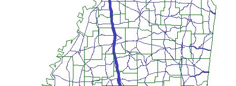
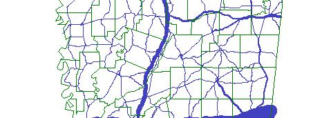
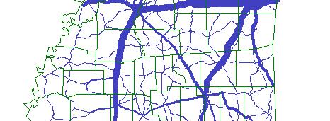
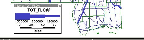
44 Figure 4-12 Wood and Wood Products in the State of Mississippi (E-I) (based on tons) Figure 4-13 Wood and Wood Products in the State of Mississippi (I-E) (based on tons) 37

45 The commodity flow characteristics for other commodity types can also be generated from the model. From the figures shown above, we can see that interstate highways in the state serve as the major transportation means for transportation commodities for the state. These results are consistent with the actual commodity flows in the state. Also, since we use shortest path assignment algorithm, links with higher speed have better attraction ability when comparing to other links. Thus interstate highways tend to carry much more tonnage of commodities than other highway types. 4.8 Conversion from Commodity Flows to Truck Trips The conversion of commodity flows to truck trips is complicated due to the presence of empty and partially loaded vehicles. Vehicle loads for different commodities are also different [12]. The Indiana model converts flows to vehicle units using load factors obtained from the Rail Waybill data. The researchers assumed that trucks would carry 40% of the load carried by railcars [38]. The conversion factors are specific to each commodity group but do not address different types of vehicles. The South Carolina model developed commodity-specific estimation of the portion of tonnage carried in each truck weight class and the average truck payload for each weight class [39]. The estimates were developed using data from the federal Truck Inventory and User Survey data and some truck origin/destination survey data. The method used in the State of Iowa is commodity and vehicle specific [12]. The model converts commodity weight into a number of annual trucks by using average density of freight and average load per truck. Empty loads were added to the network in a separate step. The Wisconsin model used the TRANSEARCH database data on tons per truck carried based on different commodity. The method used in this model is a combination of the Iowa and South Carolina methodologies. In the Iowa model, the Iowa Truck Survey is used to determine the two most common trailer types for each commodity group, as well as the average total weight of the vehicle and load carried by truck [12]. Because specific survey data is unavailable in the State of Mississippi, the VIUS database is used to estimate the composition of different truck types carrying different commodity groups. The truck capacity was obtained mainly from the VIUS database and a book titled Intermodal Freight Transportation by Gerhardt Muller [40]. The density of the cargo carried by trucks is estimated from the book titled A Shipper s Guide to Stowage of Cargo in Marine Containers [33]. The methodology is shown in Figure

46 1997 VIUS Vehicle Distribution by Commodity Group Vehicle Size by Truck Type Truck Capacity by Truck Type Cargo Density Database Average Density of Different Commodity Group VIUS Code Matching with SCTG Code SITC Code Matching with SCTG Code Payload of Different Truck Type by Commodity Vehicle Distribution by Commodity Group Payload Determination Traffic Assignment Results Convert to Truck Trips Estimate the expansion factors Apply expansion factor for empty and unloaded vehicles Truck Trips by truck type on network Truck Trips Conversion 1997 VIUS Estimate Yearly Truck Usage ADTT Truck Trips Model Validation Compare Truck Trips with Ground Counts Figure 4-14 Methodology for Converting Commodity Flow to Truck Trips 39

47 The process is divided into three basic phases: payload determination, truck trips conversion, and model validation. The procedures are as follows: 1. Determine the composition of vehicle types used to transport different commodities based on the VIUS database. 2. Determine the vehicle size distributions of different truck types and the capacity of different truck types. 3. Estimate the density of different commodity group transported by the vehicles. 4. Estimate average load of selected commodities in trucks. 5. Convert assigned freight flow to truck units based on data generated in step Estimate the expansion factor by commodity to take consideration of the empty and unloaded vehicles using VIUS database. 7. Estimate yearly truck usage using VIUS database. 8. Convert annual truck trips to ADTT and compare them with ground counts to validate the model. Steps 1 through 4 are classified as payload determination component, steps 5 and 6 are classified as truck trip conversion component, and steps 7 to 8 are classified as model validation component. The detail descriptions of each component are discussed in the following sections Payload Determination Truck Capacity Determination The number of trucks by truck type, classified by the vehicle size in VIUS is used to determine truck capacity. There are some V s and S s in the database. The V s represent less than 50 vehicles. They are assumed as 0. The S s are calibrated by the method in which the difference between the total number of trucks and sum of the number of different truck type is divided by the number of V s in the specific category. where, V T V= T j j n Tij i= 1 N (4-6) = the V s value; = total number of trucks in j vehicle size category; T = number of trucks for different truck type in j vehicle size category for j truck type i; i = type i truck; n = the number of truck types in j vehicle size category; N = number of Vs in j vehicle size category. The vehicle size in the VIUS database is classified into several ranges of lengths as shown in Table 4-9. Average length in each category was used in the analysis. The product of truck width and truck height is considered to be a constant, assuming to be 60 40

48 square feet as in some other studies [40]. The capacity analysis results are also found in Table 4-9. Table 4-9 Truck Capacity by Type Length (Feet) Single- Unit Trucks Single-Unit Truck with Trailer Single-Unit Truck With Utility Trailer Truck Type Combination Truck-tractor with Single Trailer Truck-Tractor with Double Trailers Truck- Tractor with Triple Trailers Less than % 0% 0.79% to % 1.79% 19.33% % 3.19% 28.0 to % 10.19% 67.37% 1.06% 0.049% 1.06% 36.0 to % 10.90% 6.99% 2.77% to % 15.91% 3.56% 2.67% or more 0.007% 61.22% 1.96% 93.50% 99.8% 95.74% Weighted Average Length Average Available Trailer Length Average Capacity (cubic feet) Note: The number in the upper part of the table represents percentage of different size of trucks in that category; According to Intermodal Freight Transportation 4 th edition by Gerhardt Muller, (the width)* (the height) of the truck can be assumed as 70 square feet; Average Capacity (Cubic Feet) = (average available trailer length)*(the width)* (the height); Pickups, panels, vans, minivans, and sport utilities are not included SCTG Code and VIUS Code Matching The classifications of commodities in CFS and that of VIUS are different and therefore, matching between the SCTG code and VIUS code is necessary. The matching process is basically a listing and comparison process. Most of the SCTG codes studied can be matched exactly with the VIUS code. The matching results are shown below in Table This matching procedure facilitates the related analysis procedures performed on the VIUS database. 41

49 Table 4-10 SCTG code and VIUS code Matching Results SCTG Code SCTG Product Name VIUS Code VIUS Product Name 04 Animal Feed and Prod of Animal Origin 30 Animal Feed 07 Prepared Foodstuffs and Fats and Oils 03 Processed Foods 12 Gravel and Crushed Stone 05 Building Materials 15 Coal 04* Mining Products 17 Gasoline and Aviation Turbine Fuel 10* Petroleum 18 Fuel Oils 10* Petroleum 19 Coal and Petroleum Products, n.e.c 10* Petroleum 20 Basic Chemicals 09* Chemicals 22 Fertilizer 09* Chemicals 24 Logs and Other Wood in the Rough 06 Logs and Other Forest Products 26 Wood Products Pulp, Newsprint, Paper, and Paperboard 31 Nonmetallic Mineral Products 32 Base Metal in Primary or Semifinished Forms and in Finished Basic 13 Lumber and Fabricated Wood Products 08 Paper Products 05 Building Materials 26 Glass Products 12 Primary Metal Products Fabricated Metal Products 43 Mixed Freight 20 Mixed Cargos Note: The product can be divided into several parts to match the SCTG code Commodity Density Estimation A Shipper s Guide to Stowage of Cargo in Marine Containers distributed by U.S Department of Transportation is used to determine the average density for each commodity group [33]. The commodity density information in the book is classified based on Standard International Trade Classification Index Division (SITC). To obtain the density on SCTG code, the SITC code was matched with SCTG code. The matching results and the commodity density estimation results are found in Table The results can be used to determine payload matrix of commodity by truck type Determination of Average Load Weight of Each Truck Type Based on the information derived from Tables 4-9, 4-10, and 4-11, the average payload is determined for all commodities by truck type and the results are shown in Table 4-12 (before payload limit consideration) and Table 4-13 (after payload limit consideration). During this process, the weight limit regulations enacted by Federal Highway Administration and Mississippi Department of Transportation were referenced. Any total vehicle weight (including payload) from our derivations that exceeds this amount was adjusted to the weight limit. 42

50 Table 4-11 Commodity Density Carried by Truck SCTG Code 4 7 Product Name SITC Code Animal Feed and Prod of Animal 8 Prepared Foodstuffs and Fats and Oils 9 Product Name Density (LB/Cu.Ft) Average Density (LB/Cu. Ft) Feeding-Stuff for Animals Miscellaneous Food Preparations * Concrete Brick / Block Gravel and Crushed Stone 66-2 * Glazed Brick / Block Coal 32 Coal, Coke & Briquettes Gasoline and Aviation Turbine Fuel 34 Gas, Natural & Manufactured Oil-Seeds, Oil-Nuts and Oil Kernels Fuel Oils 55 Essential Oils & Perfume Products Petroleum & Petroleum Coal and Petroleum Products, n.e.c Basic Chemicals 59 Products 50 Mineral Tar & Crude Petroleum Chemicals Chemical Elements & Compounds 64 Chemical Materials & Products Fertilizer 27 Crude Fertilizers & Crude Materials Logs and Other Wood in the Rough 24 Wood, Lumber and Cork Furniture 7 26 Wood Products 63 Wood & Cork Manufactures Pulp & Waste Paper Pulp, Newsprint, Paper, and Paperboard 64 Paper, Paperboard & Manufactured Thereof Nonmetallic Mineral Products 66 Non-Metallic Mineral Manufactures Base Metal in Primary or Semi-finished Forms and in 69 Manufactures of Metal Finished Basic 67 Iron & Steel Mixed Freight 89 Miscellaneous Manufactures Articles NEC Note: * Represents that one sub-group of 66-Non-Mental Mineral Manufactures; SITC stands for Standard International Trade Classification Code. 43

51 Table 4-12 Payload by Truck Type for Different Commodities (Before Payload Limit Consideration) SCTG Code Product Information Product Name Animal Feed and Prod of Animal Prepared Foodstuffs and Fats and Oils Gravel and Crushed Stone Average Density Singleunit Trucks Single-unit Truck with Trailer Average Payload by Truck Type Trucktractor with Single-unit Truck with Single Utility Trailer Trailer Trucktractor with Double Trailers Trucktractor with Triple Trailers Coal Gasoline and Aviation Turbine Fuel 18 Fuel Oils Coal and Petroleum Products, n.e.c 20 Basic Chemicals Fertilizer Logs and Other Wood in the Rough 26 Wood Products Pulp, Newsprint, Paper, and Paperboard 31 Nonmetallic Mineral Products 32 Base Metal in Primary or Semi-finished Forms and in Finished Basic 43 Mixed Freight Payload Limit

52 Table 4-13 Payload by Truck Type by Commodities (After Payload Limit Consideration) SCTG Code Product Information Product Name Average Density Animal Feed and Prod of Animal Prepared Foodstuffs and Fats and Oils Singleunit Trucks Average Payload by Truck Type Singleunit Truck tractor with tractor with Truck- Truck- Single-unit Truck with with Single Double Utility Trailer Trailer Trailer Trailers Trucktractor with Triple Trailers Average Payload by Commo -dity Gravel and Crushed Stone Coal Gasoline and Aviation Turbine Fuel 18 Fuel Oils Coal and Petroleum Products, n.e.c 20 Basic Chemicals Fertilizer Logs and Other Wood in the Rough 26 Wood Products Pulp, Newsprint, Paper, and Paperboard 31 Nonmetallic Mineral Products Base Metal in Primary or Semi-finished Forms and in Finished Basic Mixed Freight Weighte d Average Note: The unit of the average density is (lb/cu. Ft); Commodities included are top 15 in the State of Mississippi; Truck classification is based on the VIUS classification system. Pickups, panels, vans, minivans, and sport utilities are not included. From Tables 4-12 and 4-13, weighted average of payload in the State of Mississippi is determined to be lb, or 17.5 tons per truck. 45

53 Truck Distribution Estimation by Commodity Group The data describing the number of trucks by truck type on primary commodities carried was used. The V s and S s were calibrated by the similar methodology described in the former sections. The information was converted to SCTG code-based grouping by referring the matching results of VIUS code and SCTG code. The results of the procedure are shown in Table Table 4-14 Truck Type Distribution by Commodity VIUS Code Product Name Singleunit Trucks* Single-unit Truck with Trailer* Single-unit Truck with Utility Trailer* Truck Type Trucktractor with Single Trailer* Truck tractor with Double Trailers* Trucktractor with Triple Trailers* 30 Animal Feed 91.82% 0.42% 2.46% 4.93% 0.35% 0.01% 3 Processed Foods 70.99% 0.44% 0.51% 27.00% 1.06% 0.00% 5 Building Materials 85.98% 1.84% 3.26% 8.32% 0.60% 0.00% 4 Mining Products 66.02% 2.76% 1.14% 28.13% 1.95% 0.00% 10 Petroleum 79.60% 2.24% 1.10% 16.51% 0.55% 0.00% 9 Chemicals 88.61% 0.30% 1.15% 9.64% 0.30% 0.00% 6 Logs and Other 68.58% 2.43% 6.50% 22.04% 0.42% 0.02% Forest Products 7 Lumber and 87.53% 0.97% 2.58% 8.76% 0.17% 0.00% Fabricated Wood Products 8 Paper Products 81.17% 0.24% 0.00% 17.57% 0.97% 0.06% 5 Building Materials 86.02% 1.84% 3.25% 8.30% 0.59% 0.00% 26 Glass Products 88.57% 0.00% 0.00% 9.47% 0.00% 1.95% 12 Primary Metal 75.81% 1.30% 0.81% 21.59% 0.49% 0.00% Products 13 Fabricated Metal Products 86.20% 0.61% 3.51% 9.30% 0.38% 0.00% 20 Mixed Cargos 73.60% 0.33% 0.00% 21.08% 4.55% 0.44% Note: Source Vehicle Inventory and Use Survey table for the U.S trucks by truck type on primary products carried. *Pickups, panels, vans, minivans, and sport utilities are not included. Results from this analysis show that single unit trucks are the dominant types of trucks hauling commodities in Mississippi. This percentage distribution in the state can be used for other analyses such as estimating distribution of trucks on different types of highways Truck Trips Conversion Truck trips conversion procedure is based on information on the estimated empty factors, average payload, and truck distribution by commodity. Details are discussed in the 46

54 following sections. The expansion factors estimation procedure can be improved with more information on the transportation and economic condition of surrounding states Estimation of Expansion Factors Some trucks on the network carry partial or empty payloads. However, ground counts include full, partially loaded, and empty trucks. The empty truck issue was not addressed in the assignment method and in the conversion process. According to Iowa State s model, the expansion factors were estimated using commodity characteristics [12]. The factor captures the likelihood that a particular commodity is backhauled. According to the Iowa State s Model, a factor of 2.0 indicates that no backhaul is present all vehicles must return empty. A factor of 1.0 indicates the presence of backhaul - the returning vehicle can be used to haul another commodity. A factor of 1.5 was used to account for vehicles that may have an opportunity for a backhaul in some instances, but not in all the situations. The sensitivity of the model output to these assumptions is analyzed during the model validation process. Detailed information of the expansion factors in this study is presented in Table Table 4-15 Expansion Factors SCTG Code Product Product Name Expansion Factors by Truck Type 04 Animal Feed and Prod of Animal 07 Prepared Foodstuffs and Fats and Oils 12 Gravel and Crushed Stone 2 15 Coal 2 17 Gasoline and Aviation Turbine Fuel 2 18 Fuel Oils 2 19 Coal and Petroleum Products, n.e.c 2 20 Basic Chemicals 2 22 Fertilizer 2 25 Logs and Other Wood in the Rough Wood Products Pulp, Newsprint, Paper, and Paperboard Non-metallic Mineral Products 2 32 Base Metal in Primary or Semi-Finished Forms and in Finished Basic 2 43 Mixed Freight

55 Truck Trips Conversion The conversion from tonnage to trips was done after traffic assignment instead of before. By using an all-or-nothing assignment, it makes no difference between the two methodologies. The conversion to number of vehicles by truck type was accomplished by using the following tables developed in the former sections and adjusted by traffic assignment results [12]. o Table 4-13 Average load weight of each vehicle type; o Table 4-14 Truck distribution by commodity; o Table 4-15 The expansion factor for the treatment of empties. The procedures of the conversions are: 1. The number of trucks for transporting a specific commodity is determined by dividing assigned commodity tonnage by average load for the specific commodity. 2. Based on the truck distribution, the number of trucks by truck type is determined for each commodity group. 3. Total number of truck flows is determined by expanding the commodities to accommodate the excluded commodities during the analysis. The formulas used in the process are: N j = n ( i W j W ) / n ij (4-7) where, N j = the annual total number of all vehicles for transporting commodity j; W j W ij = the annual weight of commodity j assigned to link (tons); = the average weight by truck type i for transporting commodity j; n = the number of truck types studied. N = N * P * X (4-8) ij j ij i where, N ij = The number of trucks for transporting commodity j using truck type i; N j = the annual total number of all vehicles for transporting commodity j; P ij = the percentage of truck type I for transporting commodity j; X i = the vehicle expansion factor for empty truck type i. 48

56 4.8.3 Model Validation Yearly Truck Usage Estimation To convert the annual truck trips to average daily truck traffic counts (ADTT), many researches recommend that the annual number of vehicles be divided by 260 days [41]. Many other researches suggest that weekdays are assumed as a whole day, while weekends are considered as 0.44 work days [42]. As such, the number of working days is considered to be 306 per year [43,38]. In our study, the working days per year for the trucks are obtained from VIUS database. A table in VIUS describes the weeks operated by trucks of different type. The V s and S s are estimated using the similar method described before. From the analysis, the average number of days for a specific truck type is obtained. The analysis results are presented in Table The analysis results are truck type specific, and the average days operated of these trucks are 288 days, which is consistent with many research results [38,41,42,43]. The method used here can be justified using the process of calibrating and validating traffic assignment results, which will be discussed in 4.9 of this chapter. Table 4-16 Estimate Yearly Truck Usage by Truck Type Weeks Operated Weeks Operated Used for Calculation Singleunit Trucks Single-unit Truck with Trailer Single-unit Truck with Utility Trailer Truck Type Combination Truck-tractor with Single Trailer Truck-tractor with Double Trailers Trucktractor with Triple Trailers Less than 1 week % 2.41% 1.03% 1.62% 1.36% 0.00% 1 to % 5.09% 4.25% 1.72% 1.15% 0.00% 5 to % 5.27% 6.94% 2.40% 1.88% 1.22% 9 to % 3.42% 8.23% 2.59% 1.56% 0.00% 13 to % 2.96% 3.72% 1.97% 1.36% 4.88% 17 to % 2.22% 4.51% 1.95% 0.94% 1.22% 21 to % 6.75% 3.58% 2.73% 1.77% 1.22% 25 to % 5.74% 5.08% 3.60% 2.71% 7.32% 29 to % 5.18% 3.67% 2.62% 1.25% 1.22% 33 to % 6.57% 4.39% 3.07% 1.77% 1.22% 37 to % 11.47% 5.43% 4.71% 3.96% 3.66% 41 to % 7.49% 4.38% 6.51% 3.44% 3.66% 45 to % 7.49% 10.86% 15.18% 5.11% 1.22% 49 to % 27.94% 33.94% 49.34% 71.74% 73.17% Average Weeks Operated Average Days Operated Note: Pickups, panels, vans, minivans, and sport utilities are not included 49

57 4.8.4 Discussion on Truck Trips Conversion This study demonstrates a feasible methodology for using VIUS database to convert assigned commodity flows on each link in the network to numbers of trucks by truck type. The average loads for trucks are compared to other sources, such as the data reported in the Iowa model, with very positive results. The aforementioned methodology was a basis for studying freight movement in Mississippi. For future projects, the following areas need to be looked into: 1. All the truck information is based solely on data for entire U.S. If different sates data are available and used to determine the number of trucks by different truck type, the information on truck will be much more accurate; 2. The vehicle capacity analysis process can be strengthened with more robust data sources and better matching process between different classification scheme (i.e. the matching process of SCTG-VIUS and SCTG-SITC can be refined to get better results). 4.9 Model Validation and Calibration The traffic assignment results of I-I, E-I, I-E, and E-E O&D pairs were combined to get the truck volume on each segment of State Highways, US Highways, and Interstate Highways in Mississippi (Figure 4-15 shows the ADTT in the state). The 1997 truck counts provided by the Mississippi Department of Transportation were used to validate the aforementioned methodologies. 50

58 Figure 4-15 Average Daily Truck Traffic (ADTT) in the State of Mississippi The validation procedure is as follows: 1. The truck flows for those commodity types that were not analyzed individually were determined using an expansion factor; 2. Some of the model volumes are grouped together to match the available truck counts data; 3. Trucks are broken down into different configurations of types; 4. Volumes from the model analysis were compared to the ground truck counts. The comparison between model results and ground truck counts are presented in Table Figure 4-16 shows the comparison results at selected locations of the state network. The index information of those locations along major highways is presented in a separate figure, Figure 4-17, to facilitate references. The results show good agreement between ground truck counts and model volumes on the identified links of interstate highways, U.S. Highways and State Highways (with a weighted error margin of less than 30%). Although ground counts database may have estimate error, the overall comparison error is within the acceptable limit of model error, and is consistent with other studies in other states [6,7]. Like other studies conducted in other states, discrepancies of certain level were observed. Almost all the model volumes are somewhat lower than the ground truck counts except on the Interstate 55. Some explanations and discussions are provided as follows: 51

59 o The city selection methodology may have affected the final analysis results on the interstate highway 55. Memphis is selected as one of the representative cities in the State of Tennessee. Memphis has one of the biggest international freight airports and is located just north of the State of Mississippi. Baton Rouge, New Orleans, and Lafayette are selected as the representative cities in the State of Louisiana. Those cities are close to each other and all of them are located just to the south of the State of Mississippi. The goods transported between Memphis and the three cities in Louisiana accounts for a large percentage of the south-north freight movement, and were assigned to I-55 due to its capacity & speeds. This is probably the reason that the model overestimated the flow on Interstate 55. o The industry coverage of the CFS data has an effect on the model volume results as well. According to CFS report, the 1997 CFS survey coverage excludes establishments classified as farms, forestry, fisheries, most establishments in retail, and some other establishments [1]. This may affect the results to certain degree as the State of Mississippi is primarily an agriculture state. In addition, the 1997 CFS survey does not include the shipments that are traversing the U.S from a foreign location to another foreign location and the shipments form a foreign location to U.S location. With Port of New Orleans located just south of the state border, flows from international trade may be underestimated. Those may have been some of the reasons that volumes from the model are lower on routes other than I

60 Table 4-17 Comparison Results (Model Results vs. Ground Counts) COUNTY LOCATION ID LENGTH NAME TYPE ADTT GROUND COUNTS COMPARISON INDEX DIFF. (GROUND COUNTS- ADTT) PERCENTAGE OF DIFF. (DIFF./GROUND COUNTS) HANCOCK I MI W OF MS I10 Interstate % HARRISON I MI W OF I I10 Interstate % JACKSON I MI E OF MS I10 Interstate % WARREN I MI W OF WISCONSIN AVE I20 Interstate % HINDS I MI W OF NATCHEZ TRACE I20 Interstate % HINDS I MI E OF I I20 Interstate % LINCOLN I MI N OF BROOKWAY BLVD I55 Interstate % MADISON I MI N OF US I55 Interstate % DESOTO I MI N OF TATE COUNTY LINE I55 Interstate % PERAL RIVER I MI S OF MS 43W I59 Interstate % PEARL RIVER I MI N OF MS I59 Interstate % 53

61 FORREST LAMAR JASPER CLARKE HINDS HINDS LEAKE WINSTON WINSTON LAUDERDU WALTHALL COPIAH LAUDERDU I MI E OF LAMAR COUNTY LINE I MI N OF US 98 I MI S OF CLARKE COUNTY LINE I MI N OF MS 18 MS MI W OF TIMBERLAWN ROAD MS MI E OF RIDGEWOOD MS MI SW OF ATTALA COUNTY LINE MS MI N OF MS 395 MS MI N OF MS 395 MS MI N OF PINE LN MS MI N OF SALEM MS MI NW OF MS 28 MS MI E OF NEWTON COUNTY LINE I59 Interstate % 1 I59 Interstate % 19 I59 Interstate % 8 I59 Interstate % 21 S18 State Route % 1 S25 State Route % 18 S25 State Route % 6 S25 State Route % 10 S25 State Route % 7 S25 State Route % 9 S27 State Route % 14 S27 State Route % 12 S29 State Route % 54

62 DESOTO MS MI W OF MARSHALL COUNTY LINE S302 State Route % ATTALA MS MI S OF NATCHEZ TRACE PKWY S35 State Route % MARION MS MI N OF LOUISIANA STATE LINE S35 State Route % LAUDERDALE MS MI S OF KEMPER COUNTY LINE S39 State Route % LEE OLD US MI S OF NORTH GREEN STREET S145 State Route % YAZOO US MI S OF MS U49W US Route % SUNFLOWER US 49W 3.2 MI N OF MS U49W US Route % KEMPER US MI S OF SCOOBA US45 US Route % LEE US MI E OF SHANNON US45 US Route % FORREST US MI NE OF AIRPORT ROAD US49 US Route % FORREST US MI N OF I US49 US Route % MADISON US MI N OF MS US51 US Route % WARREN US MI N OF I US61 US Route % 55

63 WARREN SHARKEY BOLIVAR DESOTO DESOTO LEE SUNFLOWER WAYNE LINCOLN JACKSON PIKE PERRY HIGHWAY SYSTEM US MI N OF MS US MI S OF MS US MI S OF MS 444 US MI S OF TENNESSEE STATE LINE US MI SE OF MS 302 US MI W OF US 45 US MI E OF WASHINGON COUNTY LINE US MI W OF PINE STREET US MI W OF LAWRENCE COUNTY LINE US MI E OF MS 611 US MI W OF WALTHALL COUNTY LINE US MI E OF FORREST COUNTY LINE US61 US Route % 6 US61 US Route % 15 US61 US Route % 3 US61 US Route % 7 US78 US Route % 4 US78 US Route % 6 US82 US Route % 15 US84 US Route % US84 US Route % 0 US90 US Route % 11 US98 US Route % 7 US98 US Route % % 56

64 Figure 4-16 Comparison between ground counts and model results 57

65 Figure 4-17 Major locations index used in comparison 58

66 5 FREIGHT FLOW FORECASTING Using methodologies and procedures developed for the based year, freight forecasting can be performed based on future economic data. The same indicators of transportation attractions and productions are used in the forecasting: population data are used to forecast the attractions, while employment data are used to estimate productions. 5.1 Economic Data Population data and employment data are obtained from Complete Economic and Demographic Data Source (CEDDS). The CEDDS data contains time series data for future years Population Data Population data used for transportation forecasting in this study was obtained from Complete Economic and Demographic Data Source (CEDDS) data set distributed by 2001 Woods & Pool Economics, Inc [44]. CEDDS contains data and projections for all counties, states, and regions in the U.S. through the year Employment Data Employment data used for transportation forecasting in this study was also obtained form CEDDS data set. Since the commodity classification in CEDDS data set is more general than what was used in base year study. All the commodities studied in base year analyses (four digit SIC category) were classified into commodity categories in CEDDS data set (two digit SIC category). The commodity category matching results are presented in Table Methodology for Forecasting The same indicators of production and attraction as in the disaggregation process of based year study were used to forecast the commodity flow in the future years. The base year (1997) county production and attractions, along with the projected economic data for future years, were used to forecast the future commodity flow in the State of Mississippi, including the going out, within, coming into and through movements. The future years considered in the study include 2005, 2010, and The projection method used is similar to the one by the Virginia Transportation Research Council, as described in Equation 5-1 [22,23]. Similar formulas are used to project freight destinations, using the forecasted indicator of attraction. In the study, the indicator of production increase percentage is still based on employment increase. Similarly, the indicator of attraction increase percentage is based on population increase for the specific future year in study. 59

67 where, TO kif TO kib IP kif IPkif TO kif = TOkib * (5-1) IP Kib = tons of commodity k originating in i in the future year; = tons of commodity k originating in i in the base year; = indicator of production for commodity k in TAZ i in the future year; IP kib = indicator of production for commodity k in TAZ i in the base year; i = traffic analysis zonei. Table 5-1 Matching between SCTG Code and Two Digit SIC Code SCTG Code SCTG Name Animal Feed and Prods. of Animal Origin, n.e.c. Other Prepared Foodstuffs and Fats and Oils SIC Code 20 Basic Chemicals 2800* 22 Fertilizers 2800* 25 Logs and Other Wood Products in the Rough SIC Name SIC Category 2040 Grain Mill Products Manufacturing (20--) 2000 Food and Kindred Products Manufacturing (20--) Chemicals and Allied Products Chemicals and Allied Products Manufacturing (20--) Manufacturing (20--) 2410 Logging Manufacturing (20--) 26 Wood Products 2400 Lumber and Wood Products Manufacturing (20--) Pulp, Newsprint, Paper and Paperboard Base Metal in Primary or Semi-finished Forms and in Finished Basic Shapes 2600 Paper and Allied Products Manufacturing (20--) 3400 Fabricated Metal Products Manufacturing (20--) 12 Gravel and Crushed Stone 1440 Sand and Gravel Mining (10--) 15 Coal 1400* 17 Gasoline and Aviation Turbine Fuel 18 Fuel Oils Non-metallic Mineral Products 1400* 19 Coal and Petroleum Products n.e.c. Non-metallic Minerals, except Fuels Mining (10--) 1300 Oils and Gas Extraction Mining (10--) 5170 Crude Petroleum and Natural Gas Non-metallic Minerals, except Fuels Petroleum and Petroleum Products 43 Mixed Freight 4700 Transportation Services Mining (10--) Mining (10--) Wholesale Trade (50- -) Transportation and Public Utilities (40--) After production and attractions were estimated, the same procedures of base year studies were performed for the future forecasted years respectively (2005,2010, and 2020). In this study, the traffic assignment procedure was only performed on the total commodity 60

68 flow in the state (I-E, E-I, I-I) instead of by specific commodity type due to the limited time available for the research. Base Year Study Base Year O&D (E-I, I-E, I-I) Forecasted Economic CEDDS Data by SIC Commodity (2005,2010, and 2020) Forecasted Economic Data based on SCTG Code Forecasted O&D Data by SCTG Code Matching two digit SIC Code and SCTG Code Forecasted O&D Data for All Commodity Traffic Assignment Base Year Through Traffic Estimated Forecasted Through Traffic Forecasted Commodity Flow on Each Link of the Network Conversion Factors from Commodity Flow to Truck Trips in the State Forecasted Number of Trucks on Each Link Figure 5-1 Forecasting Procedures Through traffic in the state is based on the traffic assignment results excluding the State of Mississippi in U.S. OD table. Theoretically the through traffic can be estimated by forecasted U.S. OD table, however to get forecasted U.S. OD table, procedures of transportation planning in the united states have to be performed. This is out of the scope of this study. Through traffic in the state is based on the traffic assignment results excluding the State of Mississippi in U.S. OD table. Theoretically the through traffic can be estimated by forecasted U.S. OD table, however to get forecasted U.S. OD table, procedures of transportation planning in the united states have to be performed. This is out of the scope of this study. The through truck traffic was estimated to increase 50% percent in future years. So the effect of this increase was also incorporated. If time permitted, other analyses can be performed such as the increase of different commodities on a specific link in the network, the total traffic change on a specific link in the network, the efficiency evaluation of the network, and even the potential projects prioritization analysis. Please refer to Figure 5-1 for detail freight flow forecasting procedures. 61

69 5.3 Limitation of the Methodology The forecasted flow may not be an accurate estimation of the freight flow produced and attracted by the counties in the State of Mississippi due to the percentage of traffic increase may not have exactly linear relationship with the increase of the economic condition. Based on the analysis of the relationship between the traffic increase and the economic condition, a more detailed model may be developed to obtain a more reasonable forecasting of the freight flow in the future in the state. Since the public domain data from the County Business Patterns distributed by U.S Census Bureau doesn t have multiple year data readily available, and due to the time constraints, we used privately owned data from CEDDS, even though the cost to obtain CEDDS data is very minimal. This limitation can, however, be eliminated by analyzing and forecasting future time series economic data. 5.4 Forecasting Results Analyses Combining Within, Going out and Coming into assignment results, together consideration of through truck traffic, we obtained the relative increase trends on the highways. Table 5-2 and Figure 5-2 show the forecasting results. Table 5-2 Base Year and Forecasted Years Transportation Comparison Interstate State Route US Route Trend of No. of Trucks in Mississippi Change Index Interstate State Route US Route Year Figure 5-2 Trend of Number of Trucks in Mississippi 62

70 This forecasted levels of increase is in line with some US DOT estimation, but significant lower comparing to other research results [3]. Possible reasons of the low estimation are: o CFS data doesn t include shipments traversing the U.S. from a foreign location to another foreign location (e.g., from Canada to Mexico) [20]. o CFS data doesn t include shipments from a foreign location to a U.S. location [20]. o The commodity forecasting doesn t account for the transportation increase caused by the impact of Latin American Trade. Overall, the methodology is a valid and efficient way for forecasting the transportation flow in the State of Mississippi. Around 20% increase of transportation activities in the state has been estimated; the corresponding infrastructures planning and design should consider this increase. 6 FURTHER ANALYSIS USING SIMULATION TOOLS The simulation component of this research is a discrete-event macroscopic simulation. Currently, there is a lack of macroscopic transportation simulation software that is suitable for a statewide intermodal planning process. A prototype intermodal transportation planning simulation model - Virtual Intermodal Transportation Simulation (VITS) - was developed to demonstrate the feasibility of using simulation to aid in the planning and design process. It simulates the movements of trucks, trains, barges, and ships on the transportation network as well as the transference of freight between the different modes. Figure 6-1 shows a screenshot of the VITS s animation. Figure 6-1: Screenshot of the VITS Animation 63

71 The data that drives the simulation is based on the O&D data derived from earlier phases of the research process. In this prototype, performance measures such as link congestion and average traveling speed, utilization of traffic analysis zones, and the fuel efficiency have been implemented. Other performance measures and/or changes can be implemented in the future version of VITS. A simulation software package called ProModel was used in the development of the simulation component. 6.1 Simulation O&D Data Preparation The macroscopic simulation component is based on the traffic assignment results where only the arrival locations (similar to an origin) and the destination locations are needed. The simulation model covers only what s going on within the state. The following describes the locations: o For coming-into traffic, arrival locations are the locations on the Mississippi state boundaries. The centroids defined for the simulation (within the simulation traffic zones) are the destinations. o For going-out traffic, the destination locations are the boundary locations and the centroids are the arrival points. o For within traffic, the centroids for different zones represent both the arrival and destination locations. o For through-traffic, the boundary locations represent both the arrival and destination locations. The traffic analysis zones for the simulation are aggregated from the 82 counties in the state based on the population densities of the counties. The eleven traffic analysis zones are intended to distribute the traffic volumes (based on the attraction and production) evenly as shown in Figure 6-2. Based on the simulation network, traffic assignment was done for Internal-External and External-Internal freight flow. We assigned 91% of the traffic flow between the 82 counties in Mississippi and the other 47 states to the 11 traffic zones in the simulation model. A trip distribution model (Gravity model) based on the production and attraction of the 11 traffic zones and the 22 bordering points was conducted. The data preparation part will be discussed in the following sections. Figure 6-3 shows the grouping of boundary points into 10 groups numbered 12 to 21 (numbers 1 to 11 are used for naming the centroid of the 11 traffic zones). The grouping is necessary in order to reduce the complexity of the simulation OD derivation process. 64

72 Figure 6-2: Traffic Analysis Zones in the Simulation Model (County Map Generated Using TransCAD and Zones added Using a Graphics Editor) 65

73 Figure 6-3: Boundary Points and the Groupings Used for Simulation Data Preparation Assignment 66

74 Based on the truck O&D data that is derived from the CFS database, Critical Link Analysis in TransCAD was used to transfer the remote origins and destinations to the state boundary points. The commodity data associated with the State of Mississippi is transferred from remote O&D to the O&D data based on the eleven traffic analysis zones and ten entry points O&D data. Figure 6-4 shows the network used in the critical link analysis. The rail O&D data is derived following the same rules and the procedures. The water O&D are estimated based on the Comprehensive Assessment of the Ports in Mississippi report prepared by Parsons Brinckerhoff [45] with reference to the CFS database. For commodity moved by truck, population and employment as the production and attraction index was used to disaggregate the state level O&D data to county level. The assignment results from different O&D pairs were combined to get the commodity tonnage on the network in the State of Mississippi. A methodology was developed to convert the freight flows to vehicle trips to facilitate model calibration and validation. Yearly truck traffic was converted to daily truck traffic based on the truck usage information in the VIUS Database. A limitation of using the averaged daily truck traffic is that traffic pattern changes based on the hour of the day. Truck traffic is not spread out evenly over the entire 24-hour day. Therefore the simulation distributes the averaged daily truck traffic between daytime and nighttime hours as defined by the user. For rail movements, the production and attraction points are based on the rail network and major rail-served intermodal facilities as identified by Mississippi s Multiplan study. However since most railroads are privately owned and operated, the attraction and production percentage for different O&D are approximately based on the capacity of each rail-served intermodal facilities. With more specific data that includes schedules and commodities carried, more robust methodologies can be developed to supplement the incomplete data in the CFS database. For water movements, all 17 ports active in the state are identified in the network. The percentage of tonnage handled in each port is based on the Comprehensive Assessment of the Ports of Mississippi study results. The total tonnage transported in the state from CFS data analysis, along with the results from Multiplan was used to determine the water O&D. The data used for simulation focuses mainly on O&D data by different modes. The O&D data used for simulation include Truck O&D, Railcar O&D, and Barge O&D. Three intermodal scenarios are presented with the concept of transferring a certain amount of freight from single mode to intermodal, and then observing how the transference influences the performance measures used in the simulation model. 67

75 Figure 6-4: Network Used for Critical Link Analysis in TransCAD 68

76 6.2 Building of the Simulation Transportation Network Alternatives in ProModel [46] were evaluated to determine the best way of representing highway, railway, and waterway networks. Path Networks in Promodel were selected to simulate entities moving in both directions, passing, as well as speeding up and slowing down. The network in the model covers all Interstate Highways, all US Highways, and key State Highways to ensure highway freight movement coverage of over 91%. Also included are all active rail lines (includes both Class I and regional short lines) as well as the Mississippi River, Tenn-Tom waterway, and the Gulf Coast waterway. Intersections between links, which are often major towns or cities, are modeled as Promodel locations where speed calculations are made and various statistics are collected. Some statistics collected pertains to the pre-defined 11 traffic zones. The traffic zones were divided based on factors such as population density and estimated traffic densities. Key locations that include major cities and ports along the waterways are also connected to the transportation network. Information concerning the capacity (number of lanes) and speed limits are contained in an Excel spreadsheet to initialize the simulation (refer to Simulation User Guide in the appendix for more details). This allows for changes to the capacity as well as speed limits to observe the impact on the transportation system. The networks are color coded for easier reference (to represent the different classes). Refer to Table 6-1 below for more detail. The following pages show diagrams of the networks used in the simulation model (Figures 6-5, 6-6, 6-7, and 6-8). Table 6-1: Color Code for Network Links Link Color Code Red Green Brown Pink Blue Type/Classification Interstate Highways US Highways State Highways Rail Waterways The bright blue dots in those diagrams represent locations in the model that are connected to the entire network (that consists of multiple modes). They may not be shown as being connected in some figures depending upon the mode being displayed. The highways are labeled as R1, R2, R7.2, etc. The numbers corresponds to the name of the highways and the decimals, if applicable, refers to the different branch of that highway link. For more detail on the names used in the model for representing a highway segment, please refer to the Simulation User Guide in the appendix. The locations in the model are usually named after the highway link it resides on, with a unique number such as I55_M6_LOC3. The highway names are used as reference only but the last number uniquely identifies the location throughout the model and it s accompanying spreadsheets. Therefore, I55_US82_LOC5, I55_M27_LOC8, and US90_LOC73 are more simply known as locations 5, 8, and 73, respectively. In the input spreadsheet for example, the notation of O5-D73 will denote an origin at location 5 to a destination at location

77 Figure 6-5: All Highway Networks Used in Model 70

78 Figure 6-6: All State Highways and Interstates Used in the Model 71

79 Figure 6-7: All US Highways and Interstates Used in the Model 72

80 Figure 6-8: All Rail and Waterway Networks (Also Includes Interstates As Reference) 73

81 6.3 Simulation Assumptions/Considerations In this section, we review the assumptions made to build the prototype VITS. Please note that future versions of VITS can be constructed with fewer assumptions as specified by MDOT Truck Mode Assumptions o Routes are chosen at the beginning of the trip and do not change dynamically thereafter. Routing decision can be based on several criteria but in this study, the shortest path was chosen to relate to our traffic assignment procedure, which was done using shortest path in an all-or-nothing rule. o Trucks that arrive at the final destination exit the system. Less-than-truckload situations for the return trips are considered using an estimated expansion factor derived base on a study conducted by Monsere et. al. [12]. o Background traffic levels (passenger cars) for each highway network class are calculated by specifying a ratio of trucks to passenger cars. These ratios are predefined by the user for Interstates, US Highways, and Mississippi Highways. A study of passenger flows would be needed to more accurately include background traffic. o Truck speeds can be varied according to the normal distribution with the mean speed being the computed speed using the Bureau of Public Roads (BPR) traffic volume equation and a user specified standard deviation. Three standard deviations are specified for Interstates, US Highways, and Mississippi Highways. Truck speeds are governed by the BPR equation and thus are subject to the assumptions and constraints of the BPR model. o Trains and barges are always available at a location to load incoming freight from trucks for the intermodal scenario. o Specific highway link capacity reflects the number of lanes that are most prevalent on that link. o Truck traffic pattern is assumed to have a daytime duration and a nighttime duration. The beginning of the simulation signifies the beginning of the day Rail Mode Assumptions o Railcars per train vary depending on the type of locomotive used, commodity carried, gradient, and rail track conditions. As such, we use an average count of railcars per train that can be adjusted if needed. We assume, in this model that all trains consists of 60 one hundred-ton railcars. o With the limited information available on train schedules, it is possible to observe two trains in the simulation passing each other on a single track. While this is not 74

82 possible, the rail freight movement captured in the model shows only the tonnage and direction. As such, the arrivals of the trains may not match actual schedules, but are assigned randomly over the run-length of the simulation. The frequency of arrivals, however, is estimated based on annual averages (tonnage). o Regional rail lines serving industries within Mississippi appear to carry only a small percentage of the total tonnage of freight within Mississippi. With limited data, we did not consider these flows at the present iteration of the model. o Through traffic and mixed mode flows were not considered in the simulation due to limitation of data. o By assigning attraction points within the state of Mississippi to estimate the volume of freight on each assigned rail link, we assume that the train moves directly from the point of entry to the point of destination without any interruptions, such as those which may be encountered at a switching station. o All trains are moving with a full load based on user-defined characteristics (refer to the Simulation User Guide on vehicle specifications in the appendix) Water Mode Assumptions o The barges along the Tenn-Tom and Mississippi River are assumed to be breakbulk barges with an average capacity of 1500 tons. In the simulation, we model barge movements as single unit movements. o The cargo ship along the gulf coast are standardized for the simulation model as a 630 First Generation class with capacity of 1000 TEUs (Approx. 24,000 tons) o Due to data limitations, through flows and mixed-mode freight flows that involve freight were not included in the model Intermodal Assumptions Many factors affect the transfer time from one mode to another such as capacity of the terminal and traffic conditions of the surrounding area. In this model, we assume that a terminal s capacity is not a limiting factor. All loading and unloading times for the trucks, rail, barges, and ships (at exchange points) are approximated as uniformly distributed times and are user-definable in the model (mean unloading times used in the model for a barge, the entire train, and truck is 16, 16, and hours respectively). Future VITS versions can include detailed models of terminals to simulate delays based on realistic terminal capacity constraints. This feature would be particularly useful for assessing the need for upgrades at an intermodal transfer facility and how the upgrade would affect the movement of freight in the region. 75

83 6.3.5 Fuel Consumption Assumption We assume an averaged, fixed fuel efficiency for each mode. This means that trucks carrying the same load will consume the same amount of fuel whether moving in free flow speed, or moving in congested traffic. With more data available it is possible in the future to code a more accurate vehicle fuel consumption model that responds to traffic conditions and terrain variances. 6.4 Speed Calculation Highway entities (trucks) in the simulation model carry a speed attribute that governs their speed on any particular link in response to congestion. To achieve this functionality in ProModel, the BPR Equation is executed at time intervals specified by the user to update the speeds on all links in the model. Values of parameters for speed determination in the simulation model are explained in more detail in the Simulation User Guide. The BPR equation used in the simulation model is as follows: Calculated Travel Time = β x i t i 1 + α (6-1) Ci where, i = Denotes links 1, 2, 3 n; t = Free flow travel time on link i; i C = Capacity of link i; i x i = Flow on link i; α = Constant; β = Constant. A plot of speed and its relationship with the volume over capacity ratio (relating to the BPR equation) is shown in Figure

84 Congested Speed (mph) V/C Ratio Source: Volume-Delay Function and Roadway Capacity, Review of The Regional Transportation Commission of Southern Nevada s Draft Regional Transportation Plan & Transportation Improvement Plan Conformity Finding, July Figure 6-9: Interstate Speed-Flow Curve for α=0.45 and ß=7.5 Free flow travel time is based on the free flow speed for the particular link. Table 6-2 defines the free flow speeds and capacities used in the simulation model. Table 6-2: Speed Limits Highway Classification No. of Lanes (both Free Flow Speed directions) (MPH) Capacity (PCPHPL)* Interstate 2, Interstate 4, Interstate 6, Interstate 8, US Highway US Highway State Highway State Highway *Basic uninterrupted flow capacity in Passenger Cars per Hour per Lane [47] Flow is defined as the number of vehicles passing a point per unit time. In this case, the unit time is the user-defined speed update interval. According to Grady, the default α and ß values have traditionally been 0.15 and 4, respectively. He elaborated that these traditional coefficients have been replaced following more recent research. In his report, the values of 0.45 and 7.5 respectively were used to reflect upon the more current body of research [48]. We used the modern values in our simulation model. Due to the macroscopic nature of the simulation model when traffic flow is concerned, individual truck entities you see in the animation represent more than just a single truck. Although the user can change the number of actual trucks a single entity represents, this entity resolution influences the outcome of the speed calculation. This issue is not so 77

85 much of problem for a macro level simulation model as it is for a micro level simulation where the behavior of individual vehicles needs to be modeled. An entity s speed can only be set at locations where logic can be executed. In the case of using ProModel, the codes for setting the speed is implemented at the move logic section of all the locations in the model. The move logic section allows the speed to be set before the entities are released onto the highway links. This means that once the speed is set at a location, its speed can no longer change until it reaches the next location. Since the speed of the entity is directly influenced by the traffic preceding it on that link, the inability to drastically change speeds while on a link is not a significant issue for a macro level simulation model. While the data derived from the CFS Database is in terms of trucks, the capacities on the highways are expressed in terms of passenger cars. An equivalent factor of 1 truck to 2.5 passenger cars was chosen after an examination of Mississippi terrain and highway characteristics. Future versions of VITS can include more detail such as a variable factor that accounts for the terrain conditions in different traffic zones. Table 6-3, adapted from Traffic Engineering; Second Edition by Roess et. al. [42,47], was used in the estimation of the passenger car equivalent factor: Table 6-3: Passenger Car Equivalents on Extended General Highway Segments Type of Terrain Category Level Rolling Mountainous Trucks/Buses Recreational Vehicles Another issue concerns passenger car traffic on the simulation network. Since this study is focused on freight traffic, passenger car traffic is estimated as a ratio of truck to passenger cars on different classes of highways. According to the Nevada Department of Transportation, it is estimated that 10% of urban interstate highway traffic involves trucks, but the figure is higher at 31% for rural interstate highways in Our estimate for the State of Mississippi, for the interstates (considering both rural and urban) is around 25%. Similarly for other major arterials, the estimate is 9% and 21% respectively for the state of Nevada. Our estimate for Mississippi is 17% (a weighted average for both rural and urban arterials). These estimates assume that the majority of non-truck traffic can be treated as passenger car traffic [49], and the values can be easily adjusted in the model. It is feasible to include actual ground counts of passenger cars as background traffic in future versions of VITS. Animation properties for indicating slowdowns and congestions are done via several customized graphics for the truck entities. Threshold levels (expressed as a percentage of free flow speed) are used to determine when these entities change colors to reflect that they are traveling at lower speeds. Table 6-4 describes the colors codes used for the truck entity. 78

86 Table 6-4: Color Coding for Truck Entity in the Simulation Model Truck Entity Color Code Green Yellow Red Description Non-congested Medium congestion Heavy congestion Purple Trucks carrying wood products (Commodity 25 & 26) The simulation has the ability to display entities carrying different commodities using additional color codes. Figure 6-10 illustrates the color coded animation of the simulation around the Meridian region. Figure 6-10: Screenshot of Entity Color Coding 6.5 Truck Traffic Pattern To handle the varying truck traffic pattern over a 24hr day, the simulation model varies the truck traffic generation depending upon the time of the day by adjusting the time between arrivals (TBA) of trucks into the network. We define the beginning of the day to be 7am and the daytime period from 7am to 5 pm (10 hours) as default values, although the user can define the beginning of the day, the duration of the daytime hours, and the percentage of traffic during that period. Details are available on the user inputs that define the traffic pattern in the Simulation User Guide. The data preparation step provided the TBA for the trucks over a period of 24hrs. Let s denote this as TBA24, as well as TBAdt and TBAnt as the TBA for daytime and nighttime hours, respectively. Equations 6-2 and 6-3 describe the relationship between TBA24 with TBAdt and TBAnt. 79

87 TBAdt = γtba24 (6-2) TBAnt = βtba24 (6-3) where, ( 24 t1 )( c + 1) γ = ; c t1 24c β = γ cγ ; t1 t 1 = the length of the daytime period in hours; c = the ratio of truck traffic percentage during daytime hours over the truck traffic percentage during the nighttime hours. The modulus function in Promodel is used to alternate the TBA of trucks between TBAdt and TBAnt based on the system clock. These sets of equation hold true only for cases involving just two periods of daytime and nighttime. Figure 6-11 shows a plot of a highway link s traveling speed and congestion during a simulation run. Notice that the congestion plot cycles between zero (not-congested) and one (congested), showing the influence of traffic flow during daytime hours. More about this will be explained in the following section on performance measures. Traveling Speed Congestion Figure 6-11: Plot of Link Traveling Speed (Light blue) and Congestion (Dark maroon) over Time (Hours) 6.6 Performance Measures Implemented In this section we review the performance measures implemented in the prototype VITS. Additional performance measures could be implemented per MDOT specifications. 80

88 6.6.1 Link Average Speed and Congestion The traveling speed (Miles per Hour) and congestion figures for each highway link are recorded in arrays within the model. Several key links in the model are assigned variables to which the changes to both the traveling speed and congestion can be observed via dynamic plots when the simulation is running. The statistics for these travel speed and congestion variables for the links can be obtained from the standard Promodel output report at the end of the simulation run. Note that for the congestion measure, a severe congestion on a link (noted by red trucks when the model is running) is reflected by a value of one whereas the non-congested condition is simply represented by a value of zero. By doing so, an average congestion value for a link will simply denote the percentage of time the link is congested Fuel Efficiency One consideration when selecting modes is fuel efficiency, which is also closely related to vehicle emissions. While modes such as water may be slower in transit compared to trucks, concepts such as warehouse-in-transit (for which constant and reliable deliveries are required) make water a good mode choice [50]. To see the effects of mode choice on fuel efficiency, we calculate the ton-miles of each mode as well as the gallons consumed per mode. With this information, the ton-mile per gallon for the entire system can be calculated to show the impact of changes to the system. This calculation is updated every time the speed calculation is initiated, thus the updates are done every speed update time interval. Note that the gallons consumed are derived from the average fuel efficiency of that particular mode as shown in Table 6-5. Table 6-5: Fuel Efficiencies Mode Ton-Miles per Gallon Rail Highway 59.2 Waterway (Source: Fuel Efficiency in Freight Transportation, Samuel Ewer Eastman) System ton-mile are calculated as follows: System Ton-Miles per Gallon = TM G tot tot (6-4) where, TM tot is the total ton-miles transported by all the three modes and G tot is the total gallons consumed by the three modes. This value may increase or decrease as the simulation model is running, responding to chances in the mix of modes and their distance traveled during the simulation run. 81

89 6.6.3 Zone Utilization of Highways Utilization of highways in the 11 simulation TAZs are calculated by first totaling the capacities of the highways included in each zone, followed by the calculation of the ratio of total truck flow in the zone over the total capacity as shown in Equation 6-5. Utilization i = Flow Capacity i i (Equation 6-5) where, i = zone 1, 2, Note that the total flow in each zone is updated each time that truck speeds are updated (e.g. every half-hour). Since the capacities are defined as an uninterrupted flow capacity under prevailing conditions, it is possible under situations of heavy traffic to have utilizations of over 100%. Refer back to Figure 6-8 to see how a volume/capacity ratio that is approaching or exceeds 1 impacts the speed of the vehicle. In instances where a network link overlaps two zones, truck count is incremented for both zones. This condition can be avoided by establishing distinct network links within the zones. 6.7 Scenarios for Simulation Model We present a series of simplistic scenarios to illustrate the utility of a VITS planning tool. The first scenario is driven by our 1997 freight volume data and is considered the base condition. The second scenario is a future scenario where the freight volume is doubled, and the third scenario is similar to the second except that some freight is handled by intermodal shipments. A fourth scenario was also created in response to the simulated results from the third scenario. For each scenario, the simulation model is run for 60 days including 6 hours for warmup using a single replication for the purpose of demonstration. Figure 6-12 presents the links and the direction of freight flow (highlighted in blue) that are of particular interest in the scenarios. The boxes next to the highlighted links contain the link codes for reference. 82

90 R1, R2, R3, R4, R146, R5, R6 R7.2 R13, R148 R7.3, R8, R9, R10, R11 Figure 6-12: The Selected Highway Links and the Direction of Flow for Traveling Speed, and Congestion. 83

91 6.7.1 Scenario 1: Base Condition In the base condition, data from the previous steps in the study was used to drive the simulation model. The land and water modes present in Mississippi s transportation system are represented in the model to reflect current conditions. Table 6-6 summarizes the performance of the system with respect to the performance measures described earlier. Table 6-6: Summary of Results for Base Condition (Scenario 1) Simulation Zone Avg. Zone Highway Utilization Mode Avg. Daily Ton-Miles Avg. Daily Gallons % Water 490, % Rail 4,431,333 22, % Highway 171,525,000 2,897, % % % % % % % % System Ton-Miles per Gallon Note that the Average Zone Highway Utilization is the time-weighted average of the utilization for highways links that are included in the model within the particular zones. The Ton-Miles and Gallons values are the average daily values. Also, note that no passenger car information is included for the links without truck traffic, and therefore, the passenger cars count on those links is neglected. As a result, the percentage utilizations reported in the output are expected to be lower for some zones. Table 6-7 summarizes the average traveling speed (Miles per Hour) and congestion statistics for the 15 selected links in the scenario. We can see that for the base scenario, link R1 for example (an I-55 link above Senatobia), experiences very little congestion with an average traveling speed of 69 mph. The link was never congested over the simulation time. Because the average link congestion is a time-weighted average figure, a dynamic plot is useful in displaying the status of congestion (in dark maroon) for a link over the simulation run as shown in Figure This plot allows us to observe how congestion and speed changed for link R1 during the simulation. 84

92 Table 6-7: Summary of Average Traveling Speed and Congestion Statistics for the Base Condition Link Code Link Name Avg. Link Traveling Speed Average Link Congestion R1 I55_Net R2 I55_Net R3 I55_Net R4 I55_Net R146 I55_Net R5 I55_Net R6 I55_Net R7.2 I55_I20_I220_Net7 Path R13 I20_Net R148 I20_Net R7.3 I55_I20_I220_Net7 Path R8 I55_Net R9 I55_Net R10 I55_Net R11 I55_Net Traveling Speed Congestion Figure 6-13: Plot of Scenario 1 Traveling Speed (Light Blue) and Congestion (Dark Maroon) over Time (Hours) for Link R1 85

93 6.7.2 Scenario 2: Future 2X Increase in Overall Tonnage Transported In this scenario, a 2X increase in overall traffic was assumed as the future condition. This assumes that the transportation infrastructure remains identical to the base scenario and vehicle characteristics and their route choices remain constant. Again, all land and water modes are represented in this scenario. Tables 6-8 and 6-9 summarize the performance of the system. Table 6-8: Summary of Results for Scenario 2 Simulation (2X Increase) Zone Avg. Zone Highway Utilization Mode Avg. Daily Ton-Miles Avg. Daily Gallons % Water 990,045 1, % Rail 8,781,217 43, % Highway 350,766,667 5,925, % % % % % % % % System Ton-Miles per Gallon Table 6-9: Summary of Average Traveling Speed and Congestion Statistics for Scenario 2 (2X Increase) Link Code Link Name Avg. Link Traveling Speed Average Link Congestion R1 I55_Net R2 I55_Net R3 I55_Net R4 I55_Net R146 I55_Net R5 I55_Net R6 I55_Net R7.2 I55_I20_I220_Net7 Path R13 I20_Net R148 I20_Net R7.3 I55_I20_I220_Net7 Path R8 I55_Net R9 I55_Net R10 I55_Net R11 I55_Net

94 It can be clearly seen from Table 6-9 above that a future increase of 2X in traffic flow creates a more congested highway transportation system. The average traveling speed on link R1 is now 47 mph and it is congested 39% of the time (The utilization and congestion plot for this link can be seen in Figure 6-14). This is an important aspect when conducting transportation planning because the simple truck traffic average over a 24hr period excludes how traffic fluctuates over time. The system performance at such high traffic volumes is very poor, creating stop-and-go traffic conditions on this link during peak times. Traveling Speed Congestion Figure 6-14: Plot of Scenario 2 Traveling Speed (Light Blue) and Congestion (Dark Maroon) over Time (Hours) for Link R Scenario 3: Future 2X Increase in Overall Tonnage Transported with Intermodal Shifts This future scenario experiences the same increase in tonnage as described in section However, in this case, the freight normally arriving into the state by trucks through Location 1 and traveling by highway to Location 12 is changed to arrive using barges through Location 1 and travels down to Location 29 (Vicksburg) via the Mississippi River (see Figure 6-15). We assume, for the sake of discussion that the all the trucks are carrying a general commodity for Location 12 to be used by the local industry. Another assumption is that the Mississippi river and the port at Vicksburg have sufficient capacity to handle the influx of barges. It is possible that the industries (could be the plastics or packaging manufacturers) located in McComb (near Location 12) are looking into alternative modes of transportation in getting raw materials from their suppliers north of Mississippi. This is consistent with the supply chain principle where the manufacturers play an active role with their suppliers in coordinating shipments to best serve their production needs. Some industry experts have mentioned the idea of warehouse-in-transit. The slower moving barges are an excellent example of this concept. 87

95 After the trucks are loaded with freight from the barges, the journey is then resumed using from Location 29 to Location 7. From Location 7, they travel to the final destination at Location 12. Figure 6-15: Route Shift (Intermodal) for Future Scenario 88

96 Table 6-10 and Table 6-11 summarize the performance of the system for Scenario 3. Comparing this scenario with Scenario 2, we can see an increase in the System Ton- Miles per Gallon from to This is an increase of 10.63%, which is a significant difference, considering the limited intermodal use in this scenario. Table 6-10: Summary of Results for Scenario 3 Simulation (With Intermodal) Zone Avg. Zone Highway Utilization Mode Avg. Daily Ton-Miles Avg. Daily Gallons % Water 40,204,500 78, % Rail 8,781,217 43, % Highway 318,280,000 5,376, % % % % % % % % System Ton-Miles per Gallon Table 6-11: Summary of Average Traveling Speed and Congestion Statistics for Scenario 3 (With Intermodal) Link Code Link Name Avg. Link Traveling Speed Average Link Congestion R1 I55_Net R2 I55_Net R3 I55_Net R4 I55_Net R146 I55_Net R5 I55_Net R6 I55_Net R7.2 I55_I20_I220_Net7 Path R13 I20_Net R148 I20_Net R7.3 I55_I20_I220_Net7 Path R8 I55_Net R9 I55_Net R10 I55_Net R11 I55_Net

97 Looking at the average traveling speed and congestion for the highway links from Table 6-11, we can see that traffic is taken from highway designated R1, R2, R3, R4, R146, R5, and R6 when compared with the previous scenario. While this significantly reduces the congestion on Interstate 55 north of the city of Jackson (notice that R1 is no longer congested), the unloading of the barges onto truck at Vicksburg (Location 29) creates a huge traffic bottleneck for trucks moving from Vicksburg to Jackson. The result is frequent gridlock on that link R7.2 with an average speed of 35 mph, and being congested 45.76% of the time (see Table 6-11). Figure 6-16 illustrates this new dilemma, indicating the traveling speed and congestion for Link R7.2 during the simulation run. Traveling Speed Congestion Figure 6-16: Plot of Scenario 3 Traveling Speed (Light Blue) and Congestion (Dark Maroon) over Time (Hours) for Link R7.2 Realizing that link R7.2 is too heavily congested, we doubled its capacity to examine if that will help (let s call this Scenario 4). While the average traveling speed increases from 35 mph to 60 mph on this link (see Table 6-12 and Figure 6-17), it is certain that some other strategy or combinations of strategies can be applied to further improve the traffic flow on this link, since there are instances where the traveling speed is significantly below the free-flow speed. 90

98 Traveling Speed Congestion Figure 6-17: Plot of Scenario 4 Traveling Speed (Light Blue) and Congestion (Dark Maroon) over Time (Hours) for Link R7.2 Although this scenario is relatively simple, this is an example of how a simulation model can bring attention towards unanticipated results of intermodal policy changes. Table 6-12 shows the overall summary of comparison between the four scenarios. Table 6-12: Overall Summary of the Four Scenarios Scenario 1 Scenario 2 Scenario 3 Scenario 4 Avg. Daily Ton-Miles 176,447, ,537, ,265, ,437,383 Avg. Daily Gallons 2,920,366 5,970,732 5,498,258 5,551,841 System TMPG Link Codes Average Link Traveling Speed R R R R R R R R R R R R R R R

99 This overall examination yields an interesting observation. The system ton-miles per gallon is slightly lower for Scenario 4 than in Scenario 3. This can be attributed to the lowering of congestion on the critical link (in this case), R7.2, thus allowing more truck movement on that link in Scenario 4. With the increase in truck flow, the truck mode tonmiles is now slightly higher. Because the system ton-mile per gallon is calculated by taking the total ton-miles for the water, rail, and highway modes, and dividing that by the total gallons consumed, the result is a slightly lower system ton-miles per gallon value. Note that the ton-miles for the water and rail modes (in Table 6-13) are the same across Scenarios 3 and 4. The ton-miles per gallon is for Scenario 4, which translates to a 10.5% increase over Scenario 2. Table 6-13: Summary of Results for Scenario 4 Simulation (With Intermodal) Zone Avg. Zone Highway Utilization Mode Avg. Daily Ton-Miles Avg. Daily Gallons % Water 40,204,500 78, % Rail 8,781,217 43, % Highway 321,451,667 5,429, % % % % % % % % System Ton-Miles per Gallon Figures 6-18, 6-19, 6-20, and 6-21 show the close-up screenshots of the VITS animations for the four scenarios, which was taken at hour 95 of the simulation time. They show the traffic activity in the area surrounding Jackson for the four scenarios (look closely at the traffic conditions on link R7.2 between Vicksburg and Jackson across all four scenarios). 92

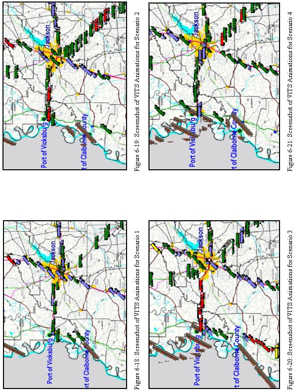
100 93