LONG-HAUL FREIGHT SELECTION FOR LAST-MILE COST REDUCTION

Transcription

1 LONG-HAUL FREIGHT SELECTION FOR LAST-MILE COST REDUCTION Arturo E. Pérez Rivera & Martijn Mes Department of Industrial Engineering and Business Information Systems University of Twente, The Netherlands INFORMS Annual Meeting 2014 Tuesday, November 11 th, San Francisco, CA

2 OUTLINE Case introduction The long-haul freight selection problem Solution approaches Mixed-Integer Linear Programming Dynamic Programming Approximate Dynamic Programming Our approach What to remember INFORMS Annual Meeting

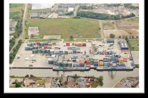
3 CASE INTRODUCTION PLANNING PROBLEM BASED IN COMBI-TERMINAL TWENTE (CTT) INFORMS Annual Meeting

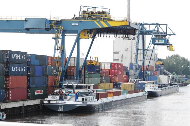
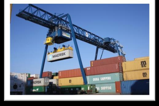
4 THE COMPANY Core business is the transportation of containers to and from Rotterdam. Long-haul of the transportation is done using barges through Dutch waterways. More than 150k containers per year (more than 300 per day). There are 30 terminals regularly visited in Rotterdam. INFORMS Annual Meeting

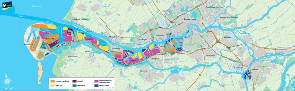
5 40 kms / 25 miles INFORMS Annual Meeting

6 THE COMPANY S COMPLAINT Barges spend around two days waiting and sailing between terminals in Rotterdam due to changes in appointments (e.g., unavailable berths, deep sea vessel arrival, etc.) INFORMS Annual Meeting

7 THE LONG-HAUL FREIGHT SELECTION PROBLEM Today a b INFORMS Annual Meeting

8 THE LONG-HAUL FREIGHT SELECTION PROBLEM Today Tomorrow Day after a b INFORMS Annual Meeting

9 THE LONG-HAUL FREIGHT SELECTION PROBLEM Today Tomorrow Day after a b INFORMS Annual Meeting

10 THE LONG-HAUL FREIGHT SELECTION PROBLEM Today Tomorrow Day after a b INFORMS Annual Meeting

11 THE LONG-HAUL FREIGHT SELECTION PROBLEM Today Tomorrow Day after a b INFORMS Annual Meeting

12 THE LONG-HAUL FREIGHT SELECTION PROBLEM Today a b Today Tomorrow Day after Tomorrow a b a b Day after a b INFORMS Annual Meeting

13 PROBLEM FORMULATION What are our problem characteristics? Discrete and finite planning horizon t T Set of freights f F Release-date r R Due-date k K Destination d D Cost per subset of destinations via barge C D R +, D D Cost of direct transport via truck B d R +, d D Capacity of the barge Q N INFORMS Annual Meeting

14 PROBLEM FORMULATION Assumptions and constraints: One barge sails per time unit (decision moment) Barge has a maximum capacity. Each freight consists of one unit (i.e., container). Each freight must be transported after its release-date and before its due-date. There is an unlimited number of trucks for the direct option. INFORMS Annual Meeting

15 MIXED-INTEGER LINEAR PROGRAMMING MODEL Non-linear! Freight goes by barge Destination is visited Freight goes by truck INFORMS Annual Meeting

16 MIXED-INTEGER LINEAR PROGRAMMING MODEL The objective can be linearized as follows: Subset of destinations is visited All subsets of the set of destinations! MILP does not include uncertainty in arrival of freights! INFORMS Annual Meeting

17 DYNAMIC PROGRAMMING MODEL One stage for each time period t T. Model s Uncertainty in arrivals between stages: Number of freights F : P F = f, f F Release-day of each freight R : P R = r, r R Due-day of each freight K : P K = k, k K Destination of each freight D : P D = d, d D All random variables are captured in an exogenous information vector W t : INFORMS Annual Meeting

18 DYNAMIC PROGRAMMING MODEL Model s states and decisions: A state S t is the collection of freights, and their characteristics, that are known at a given stage: A decision x t is the collection of freights, which have been released, that we are going to transport via barge at a given stage: INFORMS Annual Meeting

19 DYNAMIC PROGRAMMING MODEL Model s state transition between stages: A transition function S M captures the evolution of the system over the stages as a result of the decisions and the stochastic arrivals. INFORMS Annual Meeting

20 DYNAMIC PROGRAMMING MODEL A small example on how the transition function works: S t 1,d F t 1,d,0,0 F t 1,d,0,1 F t 1,d,0,2 F t 1,d,1,2 F t 1,d,1,3 F t 1,d,2,3 F t 1,d,3, x t 1,d F t 1,d,0,0 F t 1,d,0,1 F t 1,d,0, x S t 1,d W t,d S t,d - = + = F t 1,d,0,0 F t 1,d,0,1 F t 1,d,0,2 F t 1,d,1,2 F t 1,d,1,3 F t 1,d,2,3 F t 1,d,2, F t,d,0,0 F t,d,0,1 F t,d,0,2 F t,d,1,2 F t,d,1,3 F t,d,2,3 F t,d,2, F t 1,d,0,0 F t 1,d,0,1 F t 1,d,0,2 F t 1,d,1,2 F t 1,d,1,3 F t 1,d,2,3 F t 1,d,2, INFORMS Annual Meeting

21 DYNAMIC PROGRAMMING MODEL Model s costs and objective: The objective is to find a policy π that minimizes the expected costs over the planning horizon given an initial state. INFORMS Annual Meeting

22 DYNAMIC PROGRAMMING MODEL How to find this policy? Using Bellman s principle of optimality and backward induction: All possible realizations of the random variables! All possible decisions in a state! All possible states! INFORMS Annual Meeting

23 APPROXIMATE DYNAMIC PROGRAMMING MODEL Same cost and transition function as the DP model, however: A post-decision state S t x is used as a single estimator for all possible realization of the random variables. An approximated value function V t x (S t x ) for the post-decision state to capture the future costs: INFORMS Annual Meeting

24 APPROXIMATE DYNAMIC PROGRAMMING MODEL How to find the best decision for an initial state? 1 By stepping forward in time: 1. Find best decision for current state with current estimated value function of post-decision states. 2. Update the estimated value of the previous post-decision state. 3. Sample all exogenous information (in a Monte Carlo fashion), and get the new state. Repeat for a number of iterations until convergence. 1. For the comprehensive algorithm see Powell (2010) Approximate Dynamic Programming. INFORMS Annual Meeting

25 APPROXIMATE DYNAMIC PROGRAMMING MODEL Comparison between the DP and ADP (with lookup tables) models, for a small example with 7k states. In 6% of the states the ADP decisions differ from optimal. INFORMS Annual Meeting

26 OUR APPROACH Based on the ADP model with post-decision state approximation. Use basis functions for approximating the value of a state. Basis functions are specific features of a state which have a significant impact on its value. Where θ f n is a weight for each feature f F, and φ f (S t x ) is the value of the particular feature given the post-decision state S t x. INFORMS Annual Meeting

27 OUR APPROACH With regression analysis we investigate which features have a significant impact on the value of a state. In an example instance (with approx. 78k states) the following choice of basis functions explain a large part of the variance in the computed values with the DP model (R 2 = 0.94): All state variables. Number of different destinations of all freights that have the same release-day (for each release-day). Sum of all freights that that have the same release-day (for each release-day). INFORMS Annual Meeting

28 WHAT TO REMEMBER Selecting which freights to consolidate today while considering consolidation of freights in future days is important when costs depend on the combination of freights consolidated. The DP model can easily handle costs as a function of the combination of freights and uncertainty in the arrival of freights, but solving it means facing the curses of dimensionality. The ADP model overcomes the DP model dimensionality issues through the use of a post-decision state and basis functions. INFORMS Annual Meeting

29 THANKS FOR YOUR ATTENTION! ARTURO E. PÉREZ RIVERA PhD Candidate Department of Industrial Engineering and Business Information Systems University of Twente, The Netherlands INFORMS Annual Meeting 2014 Tuesday, November 11 th, San Francisco, CA