Factory Physics Analytics with applications to Project Production

Transcription

1 Factory Physics Analytics with applications to Project Production FACTORY PHYSICS is a registered trademark of Factory Physics Inc. All rights reserved.

2 Why Factory Physics Analytics? Projects are like factories Have deliverables with deadlines to meet a demand Have capacity limitations in the productive processes Can perform some production ahead of demand Have variability in both production and demand Factory Physics addresses Demand Production On time delivery Variability And how they interact

3 Factory Physics Inc Core Competence: Wrote the book on operations performance IIE Book of the Year Application of scientific principles to improving operations performance Clients European, North and South American manufacturers Global Operations Based in U.S.A Established in 2001 based on 22 years of research A consulting company with software.

4 What makes this approach different? It is scientific science relentlessly tested in industry It has software to standardize analysis and learning Rapid modeling, data obtained from existing systems Efficient frontier curves to quickly identify opportunities Where do you want to operate? Where can you operate? Ability Matrix Current State Analysis Future State Analysis Approach Speed Detail Predictive Optimal Factory Physics Analytics 2 weeks Moderate Yes Yes Six Sigma 3+ months NA No No Lean 1 week Low No No Monte Carlo Simulation 3 months+ High Yes No

5 How to Profit from Science? What to make? When to make it? How much to make? How many people and machines do I need? How much inventory should I have? Value Chain Excellence: High On-time delivery, low cost, low inventory

6 To drive profits, there are many levers a supply-chain executive must control Capacity Classes of product Ours or outside? o Standard quick-ship? o Custom? Customer Delivery What is the wait? Inventory How much, where?

7 The Project Production Manager Capacity Classes of project Ours or outside? o Standard? o Custom? Customer Delivery What is the wait? Pre-fab What, where?

8 The goal of supply chain management High Profitability The Goal Low Costs High Sales Low Unit Costs Quality Product High Customer Service High Throughput High Utilization Low Inventory Fast Response Many products Less Variability Short Cycle Time Low Utilization High Inventory More Variability Many managers bounce back and forth and call it continuous improvement.

9 Project Production no variability: demand = capacity, no waiting Due Date Available Capacity Project Time Demand Level

10 Project Production with variability: capacity > maximum demand Available Capacity Due Date Project Time Mean Demand Level Start early but no waiting

11 Project Production with variability: max dmd > capacity > mean dmd Available Capacity Due Date Project Time + wait time Mean Demand Level Start early and still late

12 Project Production with variability: little extra capacity Due Date Available Capacity Project Time + wait time Mean Demand Level Start early and very late

13 The Fundamental Factory Physics Framework Two essential components Demand Transformation Two structural elements Stocks Flows Demand Stock Production Diagram Buffers develop when variability is present. Only three buffers: 1. Inventory 2. Time 3. Capacity Production Flow WIP Stock Point Transportation Flow

14 How it Works There s physics behind Factory Physics science.

15 Demand Stock Production Production Stock Demand Production = 5 Net Inv Target Net Inv = 0 Avg Dmd = 5/day

16 More variability in production Less variability in net inventory Target Capacity buffer (base case) Capacity Production Net Inventory Inventory buffer (base case) Prod Net Inv (5) (5.00) Time buffer (base case) (10) (10.00) (15.00)

17 Low variability in production High variability in net-inventory Target Capacity buffer (base case) (5) (5.00) Inventory buffer (base case) Prod Net Inv Time buffer (base case) (10) (10.00) (15.00)

18 Buffers in Project Production Inventory pre-fabrication Prefab units Prepare materials (e.g., rebar, etc.) before hand Time quoting lead times Lead time depends on current queue. Average lead time will be less then using a constant lead time for same on-time delivery Capacity mitigate variability Recourse capacity (e.g., extra shift, weekend, overtime) No recourse = delays

19 Application of Factory Physics Analytics

20 Some Basic Factory Physics Principles Little s Law Relates basic plant performance measures WIP (CycleTime)(Throughput) VUT Equation Quantifies queueing effects Relates variability, capacity, and time buffers CT q V U t c 2 a c 2 2 e u t 1 u e Variance of Replenishment Time Demand Drives inventory and service Accounts for variability in demand AND supply Appropriate use provides predictive control and optimal performance. 2 t 2 D d 2 2 T

21 Law: Cycle time increases sharply as utilization goes to 100% Avg CT CT low CV CT hi CV Capacity Utilization You will not schedule at 100% utilization over the long term.

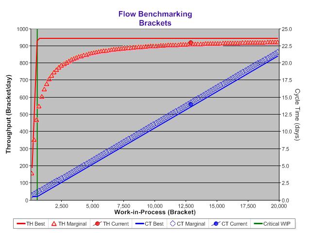
22 Performance Graph for Throughput, WIP and Cycle Time Throughput (units/day) Demand Best Case THPT Predicted THPT Best Case CT Predicted CT WIP Min. WIP Push Cycle Time (days) Best combination of Revenue, Working Capital, and Response Time ,000 Work in Process (units)

23 Average On Hand Inventory $800,000 $600,000 $400,000 $200,000 Efficient Frontiers for Stock % 95% 90% 95% 100% Fill Rate Optimal Policies

24 Average On Hand Inventory $800,000 $600,000 $400,000 $200,000 Efficient Frontiers for Stock Optimal Policies 80% 95% 90% 95% 100% Fill Rate Set Strategy. optimal Execution. RM, Kanban, Profit. and/or FG for desired customer service.

25 Best Possible Performance Goals Flows Maximum throughput with minimum cycle time Stocks Highest service level at minimum cost The final measure is cash flow.

26 Application to Project Production Pre-fab Demand Raw Material Inventory Project Production Demand The Factory Physics approach provides complete, predictive control.

27 Managing Working Capital An overview of what is possible.

28 Case I: Learning to See by Rother and Shook o Two Parts Left Bracket $10.00 Right Bracket $ 1.00 o Time in system Raw material 5 days Work in process 14 days Finished goods 12 days o Working capital for two parts Finished goods $83.5 K Work in process $91.3 K o On time delivery 88% o ~ 1 hour per day

29 Current State Map 6900 L 3700 R 12 days 14 days Source: Lean Enterprise Institute

30 Current State

31 Absolute Benchmarking

32 Overview of the Process 1. Determine the efficient frontier (i.e., min inventory investment for given service level) 2. Move to the frontier by optimizing policies Move the frontier with improvements to the operation 3 4. Move to the new frontier by re-optimizing the policies and continue 4

33 The Process Reduce Inventories Optimize Inventory Reduce WIP Little s Law Optimize lot sizes, safety stocks Repeat Reduce variability and waste

34 Step 1 Reduce Inventories Optimize Inventory Reduce WIP Little s Law Optimize lot sizes, safety stocks Repeat Reduce variability and waste

35 Optimize inventory controls No change to environment (yet!) Results Reduce inventory from $83.5K to $76.4K Increase fill rate from 88% to 89%

36 Step 2 Reduce Inventories Optimize Inventory Reduce WIP Little s Law Optimize lot sizes, safety stocks Repeat Reduce variability and waste

37 Control WIP with Little s Law CONWIP Control MTS Demand Start next job whenever WIP falls below maximum level WIP remains mostly constant CONWIP is a general pull strategy that can be used in a high-mix environment

38 Control WIP Check Throughput Optimal Lot Sizes Optimal CONWIP Level Optimal Inventory Policy MTS Demand Virtual Queue (throughput check) Active WIP Stock For make-to-stock Early completions Planned Lead Time When Virtual Queue exceeds limit Use recourse capacity or push out due dates

39 Before and after reducing WIP Cycle time = 14.0 days WIP = 91.3 K$ Cycle time = 11.9 days WIP = 77.9 K$

40 Step 2 continued Reduce Inventories Optimize Inventory Reduce WIP Little s Law Optimize lot sizes, safety stocks Repeat Reduce variability and waste

41 Before and after optimizing lot sizes Cycle time = 11.9 days WIP = 77.9 K$ Cycle time = 2.7 days WIP = 16.9 K$

42 Repeat Step 1 for improved environment Reduce Inventories Re-optimize Inventory Reduce WIP Little s Law Optimize lot sizes, safety stocks Repeat Reduce variability and waste

43 Before and after re-optimization Fill Rate = 89% FG = 76.4 K$ Fill Rate = 95% FG = 24.6 K$

44 Step 3: Reduce variability and waste Re-optimize Reduce Inventories Optimize Inventory Reduce WIP Little s Law Optimize lot sizes, safety stocks Repeat Reduce variability and waste

45 Reduce variability and waste Better balance of line. Employ standardized processes in the work place using 5S Reduce down time with FMEA and SMED. Re-optimize after improving environment

46 Before and after reducing variability and waste Fill Rate = 95.0% Fill Rate = 98% FG = 24.6 K$ WIP = 16.9 K$ Cycle time = 2.7 days FG = 5.55 M$ WIP = 3.70 M$ Cycle time = 0.60 days

47 Initial and Final States Fill Rate = 88% FG = 83.5 K$ WIP = 91.3 K$ Cycle time = 14 days Fill Rate = 98% FG = 5.55 K$ WIP = 3.70 K$ Cycle time = 0.60 days Eliminated all overtime.

48 Conclusions The improvements were dramatic The improvements were the result of changing both The policies (larger improvements) and The environment (smaller improvements) Lean and Six Sigma focus on the environment Factory Physics methods can optimize policies and identify improvement opportunities in the environment