Homophily and Influence in Social Networks

Transcription

1 Homophily and Influence in Social Networks Nicola Barbieri References: Maximizing the Spread of Influence through a Social Network, Kempe et Al 2003 Influence and Correlation in Social Networks, Anagnostopoulos et Al 2008 Feedback Effects between Similarity and Social Influence in Online Communities, Crandall et Al 2008 Community Detection and Mining in Social Media, Lei Tang and Huan Liu 2010 Learning Influence Probabilities In Social Networks, Goyal et al 2010 Sparsification of Influence Networks, Mathioudakis et Al 2011 Influence Propagation in Social Networks: A Data Mining Perspective, Bonchi 2011

2 The hidden influence of SNs We're embedded in complex and so ubiquitous social networks: how do they affect our lives? Widower effect (dying of a broken heart): when I die, my wife's risk of death can double in the first year the widowhood effect it s not restricted to husbands and wives nor to pairs of people Obesity epidemic: Every dot is a person dot size proportional to people's body size Yellow dots: clinically obese

3

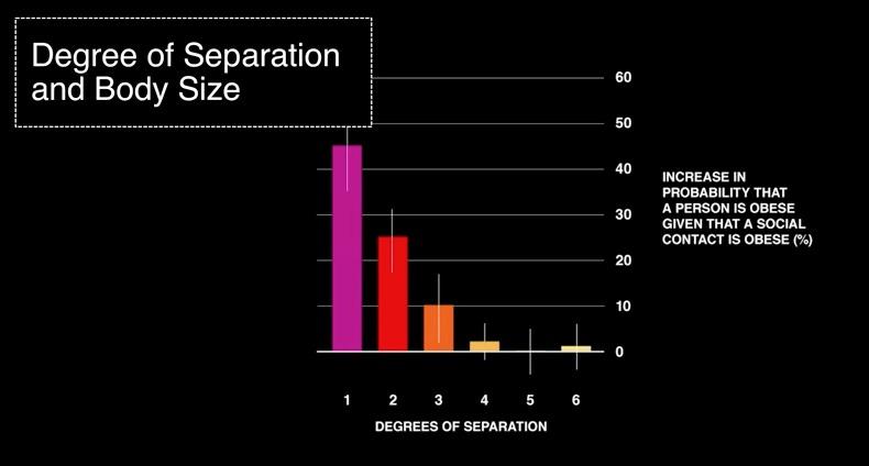
4 Analysis of the Spread of Obesity Your friend is obese: your risk of obesity is 45 percent higher Your friend's friends are obese: your risk of obesity is 25 percent higher Your friend's friend's friend is obese: your risk of obesity is 10 percent higher. Only when you get to your friend's friend's friend's friends that there's no longer a relationship between that person's body size and your own body size. What might be causing this phenomenon? As I gain weight, it causes you to gain weight I form my tie to you because you and I share a similar body size We share a common exposure to something

5 :-) :-( :-/

6 Influence and Correlation in SNs The availability of rich data from popular Social Networks makes it possible to analyze user actions at an individual level in order to understand user behavior at large How user s actions can be correlated to his/her social connections? What is the source of the correlation? We are concerned with individuals performing a certain action for the first time, e.g., purchasing a product, visiting a web-page, or tagging a photo with a particular tag After an agent performs the action, we say that the agent has become active Social correlation: for two nodes u and v that are adjacent in G, the events that u becomes active is correlated with v becoming active.

7 Models of Social Correlation Homophily: is the tendency of individuals to choose friends with similar characteristic. Individuals often befriend others who are similar to them, and hence perform similar actions Birds of a feather flock together Confounding: the correlation between actions of adjacent agents in a social network can be explained by assuming an external influence both the choices of individuals to become friends and their choice to become active are affected by the same unobserved variable Influence: the action of individuals can induce their friends to act in a similar way a user buys a product because one of his/her friends has recently bought the same product

8 Models of Social Correlation

9 Homophily: Analyzing similarity over time How does the similarity between two people vary in the time window around their first interaction with each other? An elevated level of similarity just before meeting indicates a type of selection at work, while increasing similarity following this meeting provides evidence for social influence. Average cosine similarity of user pairs as a function of the number of edits from time of first interaction, for Wikipedia Baseline: average similarity for pairs of users who have not interacted Selection Influence? Separate plots are shown for pairs of users with different activity levels (at least k edits before and k edits after the first interaction) Avg similarity pairs of user who have not interacted

10 Identifying Social Influence Identifying situations where social influence is the source of correlation is important. In the presence of social influence, an idea, norm of behavior, or a product diffuses through the social network like an epidemic. Activation Process: in each of the time steps [1,..., T] each non-active agent decides whether to become active: The probability of becoming active for each agent u is a function p(x) of the number x of other agents v that have an edge to u and are already active

11 Measuring social correlation In the influence model, each individual flips an independent coin in every time step to decide whether or not to become active Simple case: we measure this probability as a function of only one variable, the number of already-active friends We can estimate the probability p(a) of activation for an agent with a already-active friends as follows: The coefficient α measures social correlation: a large value of α indicates a large degree of correlation We estimate α, β using maximum likelihood logistic regression

12 Measuring Social correlation Ya,t: number of users who at the beginning of time t had a active friends and started using the tag at time t Ya = Σt Ya,t Na,t : number of users who at time t were inactive, had a active friends, but did not start using the tag Na = Σt Na,t We compute the values of α and β that maximize the expression

13 The Shuffle Test If influence does not play a role, the timing of activations should be independent of the timing of other agents. Let G be the social network, and W = {w1,...,wl} be the set of users that are activated during the period [0,T]. We compute Ya and Na, and use the maximum likelihood method to estimate α. We create a second problem instance with the same graph G and the same set W of active nodes, by picking a random permutation π of {1,...,l}. We compute Y a and N a and the social correlation coefficient α The shuffle test declares that the model exhibits no social influence if the values of α and α are close to each other.

14 The Edge-reversal Test We reverse the direction of all the edges and run logistic regression on the data using the new graph If the correlation is based on the fact that two friends often share common characteristics, we intuitively expect reversing the edges not to change our estimate of the social correlation significantly. Social influence spreads in the direction specified by the edges of the graph, and hence reversing the edges should intuitively change the estimate of the correlation.

15 Influence on Flickr

16 Influence Propagation in SNs A social network plays a fundamental role as a medium for the spread of information, ideas, and influence among its members The basic assumption is that when users see their social contacts performing an action they may decide to perform the action themselves

17 Diffusion Models At a given timestamp, each node is either active (an adopter of the innovation, or a customer which already purchased the product) or inactive Each node s tendency to become active increases monotonically as more of its neighbors become active An active node never becomes inactive again Time unfolds deterministically in discrete steps As time unfolds, more and more of neighbors of an inactive node u become active, eventually making u become active, and u s decision may in turn trigger further decisions by nodes to which u is connected.

18 Independent Cascade Model When a node v first becomes active, say at time t, it is considered contagious. It has one chance of influencing each inactive neighbor u with probability pv,u, independently of the history thus far. If the tentative succeeds, u becomes active at time t + 1. The probability pv,u, that can be considered as the strength of the influence of v over u

19 Linear Threshold Model A node v is influenced by each neighbor w according to a weight bv,w such that Each node v chooses a threshold θv uniformly at random from the interval [0, 1]; This represents the weighted fraction of v s neighbors that must become active in order for v to become active. In step t, all nodes that were active in step t 1 remain active, and we activate any node v for which the total weight of its active neighbors is at least θv:

20 Linear Threshold Model Assume bw,v = 1/kv and that the threshold for each node is 0.5.

21 ICM vs LTM LTM is receiver-centered ICM is sender-centered LTM s activation depends on the whole neighborhood of one node LTM, once the thresholds are sampled, the diffusion process is determined ICM is specified by a stochastic process

22 Influence Maximization Viral marketing: suppose that we have data on a social network, with estimates for the extent to which individuals influence one another, and we would like to market a new product that we hope will be adopted by a large fraction of the network The aim is to detect few influential nodes to target in order to maximize the spread on the network Suppose that we want to push a new product in the market and we are given: a social network the estimates of reciprocal influence between individuals connected in the network Influence Maximization: how should one select the set of initial users so that they eventually influence the largest number of users in the social network?

23 Influence Maximization Both the Linear Threshold and Independent Cascade Models involve an initial set of active nodes A0 that start the diffusion process σ(a) is the expected number of active nodes at the end of the process, given that A is this initial active set. Given a parameter k find a k-node set of maximum influence. Both for IC and LT it is NP-hard to determine the optimum for influence maximization but... (continue)

24 Approximated Algorithm Given a propagation model m, if σm(s) is monotone and submodular then the optimal solution for influence maximization can be efficiently approximated to within a factor of (1 1/e ε) (slightly better than 63%) Monotonicity says as the set of activated nodes grows, the likelihood of a node getting activated should not decrease Sub-modularity: the probability for an active node to activate some inactive node u does not increase if more nodes have already attempted to activate u (diminishing returns property)

25 Greedy Algorithm for IM The step 3 is #P-hard We can employ Monte Carlo simulation Heuristics to improve the efficiency of the Greedy algorithm

26 Speeding up the Greedy algorithm We aim to find a node with the maximal marginal gain Exploit the submodularity!!! σ(s {v}) σ (S) σ(s t {v}) σ (S t ) σ(s t+1 {v}) σ (S t+1 ) The marginal gain of adding a node v to a selected set S can only decrease after we expand S Suppose we evaluate the marginal gain of a node v in one iteration and find out the gain is Those nodes whose marginal gain is less than in the previous iteration should not be considered for evaluation because their marginal gains can only decrease

27 IM Process

28 IM Process How to learn influence Probabilities?

29 Learning Influence Probabilities We are given: a social graph in the form of an undirected graph G = (V, E) where the nodes V are users and (u,v) E represents a social tie between the users a relation Actions(User, Action, Time), which contains tuples (u, a, tu) indicating that user u performed action a at time tu Au Au&v Au v Av2u number of actions performed by user u in the training set number of actions performed by both u and v in the training set number of actions either u or v performs in the training set number of actions propagated from v to u in the training set. We want to learn a function p : E [0, 1] [0, 1] assigning to both directions of each edge (v, u) E the probabilities: pv,u and pu,v

30 Jaccard Index Static Models Bernoulli distribution: any time a contagious user v tries to influence its inactive neighbor u, it has a fixed probability of making u activate Partial Credit: each of the neighbors who have performed the action before share the credit for influencing u to perform that action Suppose user u performs an action a at time tu(a) and S its set of activated neighbors Flickr social network and we consider joining a group as the action

31 Continuous Time (CT) Models Influence probability may not remain constant in time The probability of v influencing its neighbor u at time t is: p 0 v,u is the maximum strength of v influencing u (static models) τv,u can be estimated as the average time delay in propagating an action from v to its neighbor u in the training set. The probability of u being influenced at time t by the combination of its active neighbors is If max {p t u(.)} θu, the activation threshold of u, we conclude that u activates

32 Learning the parameters of the IC Model The independent cascade model generates independent propagation traces The set F + α(v) of nodes that possibly influenced v are the nodes that performed action α before v and within t time The set F - α(v) of nodes that definitely failed to influence v

33 EM Algorithm The likelihood Lα(G) of the trace can be written as

34 EM Algorithm The likelihood Lα(G) of the trace can be written as where we have two contributes: 1. likelihood that at least one of the nodes in F + α(v) succeed to influence v

35 EM Algorithm The likelihood Lα(G) of the trace can be written as where we have two contributes: 1. likelihood that at least one of the nodes in F + α(v) succeed to influence v

36 EM Algorithm The likelihood Lα(G) of the trace can be written as where we have two contributes: 1. likelihood that at least one of the nodes in F + α(v) succeed to influence v 2. likelihood that the nodes in F - α(v) fail

37 EM Algorithm The likelihood Lα(G) of the trace can be written as where we have two contributes: 1. likelihood that at least one of the nodes in F + α(v) succeed to influence v 2. likelihood that the nodes in F - α(v) fail

38 EM Algorithm The likelihood Lα(G) of the trace can be written as where we have two contributes: 1. likelihood that at least one of the nodes in F + α(v) succeed to influence v 2. likelihood that the nodes in F - α(v) fail The probability values p(u, v) that maximize the total log-likelihood can be computed using the following iterative formula

39 EM Algorithm The likelihood Lα(G) of the trace can be written as where we have two contributes: 1. likelihood that at least one of the nodes in F + α(v) succeed to influence v 2. likelihood that the nodes in F - α(v) fail The probability values p(u, v) that maximize the total log-likelihood can be computed using the following iterative formula

40 EM Algorithm The likelihood Lα(G) of the trace can be written as where we have two contributes: 1. likelihood that at least one of the nodes in F + α(v) succeed to influence v 2. likelihood that the nodes in F - α(v) fail The probability values p(u, v) that maximize the total log-likelihood can be computed using the following iterative formula

41 EM Algorithm The likelihood Lα(G) of the trace can be written as where we have two contributes: 1. likelihood that at least one of the nodes in F + α(v) succeed to influence v 2. likelihood that the nodes in F - α(v) fail The probability values p(u, v) that maximize the total log-likelihood can be computed using the following iterative formula

42 Key Concepts Influence vs Selection Diffusion Models ICM LTM Influence Maximization Problem Learning Influence Weights