Implementation and process optimization of a dynamic transportation problem

Size: px

Start display at page:

Download "Implementation and process optimization of a dynamic transportation problem"

Rosemary Butler
5 years ago
Views:

1 Projektstudium an der Technischen Universität München Implementation and process optimization of a dynamic transportation problem Referent: Prof. Dr. Rainer Kolisch Lehrstuhl für Operations Management Technische Universität München Betreuer: Alexander Döge, M.Sc., TUM School of Management Dominik Eggert, Dipl. -Kfm., Founder of LIINITA Studiengang: Technologie- und Managementorientierte Betriebswirtschaftslehre, TUM BWL Eingereicht von: Daniel Bogner Lerchenauerstraße 150, München Matrikelnummer: Martina Rehklau Wildweg 3, Germering Matrikelnummer: Eingereicht am:

2 Table of Contents Table of Contents... ii List of Figures... iii List of Tables... iv List of Pseudo Codes... v List of Abbreviations... vi List of Symbols... vii 1 Introduction Problem Situation and Motivation Methodology Classification of LIINITA s Business Model Vehicle Routing Problem Heuristics and Metaheuristics Nearest Neighbor Algorithm Opt Specification of Constraints Pickup & Delivery Time Windows Evaluation of the Results Conclusion Reference List Appendices Declaration of Authorship ii

3 List of Figures Figure 1: Example Tour before 2-Opt Figure 2: Example Tour after 2-Opt Figure 3: Tours generated without PD Figure 4: Improved Tour with PD Figure 5: Map with Example Customer Distribution in Munich Figure 6: Histogram of Time Matrix Data Figure 7: Solution Overview Figure 8: Trend Chart of Waiting Time Modifications; Whole Day Figure 9: Trend Chart of Waiting Time Modifications; Core Time All presented figures are compiled by the authors of this study iii

4 List of Tables Table 1: Results of Waiting Time Modifications; Whole Day Table 2: Results of Waiting Time Modifications; Core Time Table 3: Results of Starting Time Modifications; Whole Day Table 4: Results of Starting Time Modifications; Core Time All presented tables are compiled by the authors of this study iv

5 List of Pseudo Codes Pseudo Code 1: Methodology... 6 Pseudo Code 2: Nearest Neighbor Pseudo Code 3: 2-Opt Heuristic Pseudo Code 4: Pickup and Delivery All presented pseudo codes are compiled by the authors of this study v

6 List of Abbreviations mtsp NN PD TSP TUM TW VRP VRPPD VRPTW WT Multiple Travelling Salesman Problem Nearest Neighbor Simultaneous Pickup and Delivery Travelling Salesman Problem Technische Universität München Time Window Vehicle Routing Problem Vehicle Routing Problem with simultaneous Pickup and Delivery Vehicle Routing Problem with Tim Window Constraints Waiting Times vi

7 List of Symbols a A best_improvement best_i best_j capacity currentposition d D fromikea h improvement n nextposition m matrix mindistance mintag mintravtime- Delivery P q Actual Time Set of Edges Connecting Two Vertices Double Parameter to mark Best Improvement found Integer Parameter to mark first vertex exchanged in 2-Opt Integer Parameter to mark second vertex exchanged in 2-Opt Current Vehicle Capacity Integer Parameter to mark current Request in Tour Distance or Travel Time Set of Delivery Requests within R Delivery Request Starting Time of a Tour at IKEA Double Parameter to mark Travel Time Sum of Tour Earliest Arrival Time at Pickup Request Integer Parameter to mark next Request in Tour Latest Arrival Time at Pickup Request Two Dimensional Array containing Time Matrix Integer Parameter to mark shortest Distance Boolean Parameter to mark if valid Request is found Double Parameter to mark minimum Travel Time Set of Pickup Requests within R Maximum Capacity of a Vehicle vii

8 R t toikea tourarray traveltimenn u v visited V w weight y Set of Customer Requests of a Tour Arrival Time at Customer Pickup Request Array containing Customer of a Tour Double Parameter to mark Travel Time Sum of NN Tour Travel Time of Request Earliest Start Time of Delivery Request Array depicting if a Customer has been visited Set of Customers Latest Start Time of Delivery Request Array containing Weights of all Customer Current Amount of Customers in Vehicle viii

9 1 Introduction Society has gained a special interest in environmentally related issues over the last couple of years (Mishalani et al., 2014). A range of events e.g. earth warming discussions or the increasing awareness of the carbon footprint led to this consciousness. That s why many green-minded individuals focus on purchasing products or using services from companies that produce or provide services in an ecologically and ethical responsible way. It became apparent that sustainable development on the one hand and responsible use of resources on the other hand are a key to success. At the same time, they are important factors in order to reduce the carbon footprint. Nevertheless, providing sustainable solutions in all kinds of areas in an industrialized nation as Germany is no easy task. One major part in order to ensure progression is a good infrastructure. This comes along with a tremendous need for mobility as well as flexibility. Therefore a lot of scientists from different departments design complex processes and technology to use given resources efficient. A great problem is the transportation of individuals in nowadays expanding cities with regard to eco-friendly use as well as intelligent coordination of available resources. Besides technological improvement an optimization of processes and diligent use of existing products is essential. Using the subway e.g. is a relatively green way to travel because it is powered by electricity and hundreds of people are travelling together at one time, in a minute cycle. But how many people really take a train, subway or bus frequently? Sometimes it is not enough to travel from one to another station. Sometimes it has to be faster, more relaxing and most notably an individual adjusted route with an individual adjusted time frame is needed. Car sharing is a great opportunity to apply those specific requirements. But despite all positive effects of car sharing, another inefficiency occurs: the capacities of the shared cars are mostly not fully exhausted and seats stay empty. To avoid this free capacity, people with the same destination can be grouped into one vehicle. This is what the Startup LIINITA is going to accomplish with its business model. The basic idea is to provide convenient and rapid city transportation with Minibuses that pick up and deliver people simultaneously. The assumption is to 1

10 make the best use of one vehicle s capacity while considering all customers requirements and constraints. Accordingly the passenger s locations and the desired pickup and drop off time have great influence on the generation of the routes. In this Project Study we want to implement and critically evaluate the results of this promising transportation opportunity in cooperation with LIINITA. Our goal for this study is to provide a first overview over the upcoming challenges within this complex task. In the following we want to illustrate and present the idea behind this business model in a more detailed way. Afterwards we are going to introduce problemsolving approaches as well as common heuristics to approach the current transportation problem. Thereby, the overall goal is to generate tours for vehicles that pick up and deliver several customers. These tours have to be developed under specific circumstances and should be as efficient as possible. It should be emphasized that the results present a feasible solution, but they are not necessarily optimal. 2

11 2 Problem Situation and Motivation To simplify the travelling process as well as to assure economical satisfying results, Dominik Eggert, founder of LIINITA, worked out a complex business concept. The idea is to establish a novel minibus sharing system that serves individual customer transportation needs. To launch the business model and apply it on a real life scenario, Mr. Eggert came to an agreement with an IKEA store located in the suburbs of Munich. LIINITA provides a transportation possibility for customers, who want to travel to IKEA and back. Thereby IKEA finances a part of the expenses and helps LIINITA to increase its popularity. IKEA is known to sell ready-to-assemble furniture and observed noteworthy decreases in purchasing power (Süddeutsche Zeitung, Jun 2014). One distinct factor that contributes most to this decrease is that a lot of potential customers are not able to get to a store that is located outside of the public transportation network. To counteract that, IKEA opened a facility in the City Center of Hamburg to avoid a loss of potential customers (Süddeutsche Zeitung, Jun 2014). This relocation comes along with an immense amount of planning and high costs, which the model of LIINITA tries to avoid. The idea is that people book their trips via applications on their smartphone and receive information about available trips immediately. Passengers can be picked up at a requested location in the city center of Munich and brought back from IKEA to a desired destination. Furthermore customers, who want to travel to IKEA, can decide between several overlapping thirty-minute time slots according to their preferences. If a customer e.g. wants to be picked up at 10am, three potential time windows can be considered. The first possibility is a time window from 9.30am to 10am. The second conceivable option is from 10am to 10.30am. However another opportunity is a time window from 9.45am to 10.15am. This is done in order to simplify the calculation process and assure real-time improvement. Also, long waiting periods should be avoided and thus customer satisfaction is achieved. Besides those pickup customers, there are also customers travelling back home. To serve these delivery customers it is intended that every 20 minutes a vehicle starts from IKEA and drives them back home to their chosen location. To increase 3

12 effectivity it is feasible to combine pickup and delivery customers in one route. With a maximum capacity of eight customers per vehicle, an ideal tour would be to start with eight delivery customers at IKEA, delivering them and meanwhile collecting eight pickup customers before driving back to IKEA. Of course, several constraints like destination, pickup point, individual time windows, and quantity of the request have to be considered. Therefore the actual resulting tour can vary from that ideal tour. Moreover this coordination of the simultaneous pickup and delivery procedure requires a complex examination and will be discussed in chapter In the following we want to critically evaluate heuristic strategies used to solve this particular problem. We want to ensure an improved real time automated calculation of the customer s assignment to different vehicles. The implementation of this logistical process requires a complex reflection and is done with the programming language Java. To demonstrate the appliance of the developed code and present a first solution to this complex problem, an example is used and interpreted. This example illustrates one possible day with various requests and all necessary conditions. 4

13 3 Methodology Before examining the single steps used to approach the task, this chapter provides an overview over the methodology of this project study. The process of generating the tours under specified conditions follows a certain sequence. At first an algorithm is used to create a starting solution. Therefore delivery customers are added to a trip until maximum capacity q of the vehicle is reached or there are no more delivery requests at that time left. This means at the starting time h a tour begins at IKEA with a certain number of customers in the vehicle. With arriving at a destination of a delivery request and dropping of customers, capacity in the vehicle becomes free again and the current amount of customers in the vehicle y decreases. The free capacity can then be used to gather additional pickup customers, before travelling back to IKEA. With that consideration as many pickup requests as possible are added to the single delivery tour. Remaining customers, which could not have been allocated in these combined tours, are then embedded into a single tour. Afterwards a heuristic is used to improve this starting solution. For that matter the nodes in a tour are arranged in a new order and compared to the starting solution. Here the minimization of travel times is the decisive criterion. Finally feasible amendments are applied. The following generic formulation depicts the methodology that determines the generation process and its objective function. 5

14 Methodology Sets R = {1, n} P = {1, n} D = {1, n} I = {1, n} Customer Requests Pickup Requests of R Delivery Requests of R Nodes in Tour Parameters q y i n p m p t p v d w d h maximum capacity of vehicle amount of customers in vehicle at i ϵ I earliest arrival time at p ϵ P latest arrival time at p ϵ P arrival time at p ϵ P earliest start time of d ϵ D latest start time of d ϵ D individual start time of each tour Decision Variables u r travel time of request r ϵ R Objective Function: Min z = i ϵ I u r Minimize Travel Time subject to y i q ; i ϵ I Capacity Constraint n p t p m p ; p ϵ P Pickup Time Window Constraint v d h w d, ; d ϵ D Delivery Time Window Constraint u r 0, ; r ϵ R Non-negativity Constraint Pseudo Code 1: Methodology At first the listed parameters within the named request sets have to be considered in order to define the objective function and its restricting conditions. The objective function is to minimize the travel time each customer spends in the vehicle within a tour. This tour may contain pickup, delivery or combined requests, which all have individual modified constraints affecting the customer selection. 6

15 As mentioned before the maximum capacity q of each vehicle limits the number of customers that can be served in one tour. Since the combination of pickup and delivery requests allows to serve up to 16 requests per tour, the current amount of customers in a vehicle y has to be measured. At no time within the tour, y may exceed the capacity q. Therefore the different quantities of the requests have to be adhered and applied. Moreover the time windows of the customer requests are an important condition. A time window represents the preferred pickup time for pickup customers and the preferred time of departure at IKEA for delivery customers. This are significant constraints and will be accurately explained in chapter Furthermore no customer should spend more time in a vehicle than his direct travel time to IKEA times three. This condition has been invented to avoid long travel times and increase customer convenience. For convenience this constraint is not mentioned in Pseudo Code 1 but it is implied in the developed solution. In order to analyze what influence the different constraints have on the resulting tours, alterations are done. These alterations are used to show how reasonable different constraints are and will be further explained in chapter 5. 7

16 4 Classification of LIINITA s Business Model 4.1 Vehicle Routing Problem After specifying the case of this paper, the following chapter defines the problem in terms of route optimization. In the 18th century the mathematicians Hamilton and Kirkman studied as one of the first the Travelling Salesman Problem (TSP) which is the origin of the Vehicle Routing Problem (VRP). A detailed evaluation of their work can be seen in the book Graph Theory by Biggs et al. (1976). Typical conditions for formulating a TSP are a given number of cities represented by vertices. Those vertices have to be visited and each tour starts and ends at the same node, often the depot. The distance or travel time between each vertex is known. In this paper customers represent the vertices. The task is to find the best possible way of visiting all customers while minimizing the travel time or distance at the same time. To classify, R = {r 0,,r n } is a set of customers with r 0 as the depot and A = {(g, s) : g, s R} as a set of edges connecting vertex r and vertex s. The measured non-negative travel time or distance d gs is associated with the edge (g, s) A. Further we speak of a symmetric case which means that d gs = d sg. Although the routes can diversify when distinguishing the directions, a symmetric journey is assumed. Therefore this symmetric scheme means that the travel time from a customer to IKEA and the travel time from IKEA to a customer are equal. The reason behind that is the workability of the algorithms used. Especially the applicability of the 2-Opt algorithm is influenced by that and is further discussed in chapter For further studies a modification to the code should be made in order to apply an asymmetric scheme. LIINITA presents a business model in which a vehicle starts at a depot (IKEA), visits a certain number of locations and then returns to the starting point. This is done while the travel time for the entire route is minimized. These criterions seem to be similar to those mentioned of a TSP, but it is not the final definition of LI- INITA s routing problem. Further we want to define the problem more accurately. A classical, single TSP is concerned with connecting all given vertices in one route, visiting each node only once. As here the decisive criterion to the objective function is to minimize the travel time each customer drives in the vehicle, a multiple Travelling Salesman 8

17 Problem (mtsp) may be a more appropriate definition. Within the mtsp all vertices can be allocated in different single routes with the goal to minimize the total travel time. Further a mtsp with additional capacity restrictions of different vehicles is defined as a Vehicle Routing Problem. Proposed by Dantzig and Ramser in 1959, the VRP is a combinatorial optimization problem that developed out of the necessity for route scheduling. Practically, vertices are allocated to different single routes just like within the mtsp, where every route starts and ends at the depot. The difference here is a maximum capacity of each vehicle. This capacity restriction determines whether a new vertex can be visited or not. This is exactly the problem situation of LIINITA and therefore its routing problem is not only a TSP, but can be categorized as a VRP. Additionally two different routing types have to be considered. As mentioned in the previous chapter, vehicles can either pickup customers and carry them to IKEA or deliver customers from IKEA back to a drop-off location. This affects the routing process of the VRP, because if a customer travels back from IKEA and is delivered, the vehicle has again free capacity. This gives the possibility to pick up a new customer who wants to travel to IKEA. This simultaneous pickup and delivery (PD) is important for the definition of the VRP. The other important constraint besides PD is the individual time window each customer has. Both constraints are special characteristics of the VRP and are called a Vehicle Routing Problem with simultaneous Pickup and Delivery and Time Window (Hokey, 1989). To find a satisfying solution for this difficult problem, one possibility is to use a heuristic method (Lenstra et al., 1981). This approach to the problem is discussed in the following chapter. 9

18 4.2 Heuristics and Metaheuristics Due to the fact that the VRP is obtained as a problem that is difficult to solve, finding a solution for it can be divided into two methods (The Journal of the Operational Research Society, 2002). On the one hand there are exact solution methods to optimize the outcome. This requires a runtime of the algorithm that is too extensive for this case. Since we want to find a solution in a preferably short time span the second method, which describes heuristics should be applied. Heuristics are used to find a good solution in a short time, but an optimal solution cannot be guaranteed. For the adaption on LIINITA s business model we chose to generate a solution with heuristic methods, because the goal of this first implementation is to find an applicable method and not primary to discover the optimal solution among other good performances. When considering heuristics again two types can be distinguished (Laporte et al., 2000). The first are construction heuristics like Nearest Neighbor, Sweep Method or post optimization heuristics like k-opt. Those are based on a local search for a solution. The other are metaheuristics like Genetic Algorithm or Simulated Annealing, which are based on a global search. Both describe an approximate solution to a problem. The difference is, a construction heuristic uses problem-dependent information to find a good enough solution to a specific problem. This is often only a local optimum, but can be calculated in a short time span. Metaheuristics on the other hand describe general algorithmic ideas that can be applied to a broad range of problems (El-Ghazali Talbi 2009). Moreover they try to escape from a local optimum and find a global optimal solution. As a result metaheuristics are mostly much more time consuming in the process. Before finding a local or global optimum, first a valid starting solution has to be created. Common heuristics to find a starting solution for the VRP are the SWEEP Method or the Nearest Neighbor Algorithm (NN). The SWEEP Method develops a route by following a sweep line construction. On the other hand, the NN creates a tour by adding the vertex to the route with the smallest distance to the current vertex. To generate a starting solution we chose to use the NN, because it generates a tour with nearby customers and thus a small sum of travel times, as desired, is accomplished. A more detailed overview over the NN is given in the following chapter

19 After generating a starting solution the next task is to examine if there exists an improvement. A common method to find an improvement for a solution generated by the NN is the k-opt heuristic. By exchanging k edges within the tour and reconnecting them in a different direction a new tour is developed. The new tour is then compared to the old one and the best is kept in the further process. An advantage of the k-opt is the simplicity of the algorithm. This results in a low processing time, exactly like it is aspired in the case of LIINITA. For that matter we chose to use the 2-Opt heuristic to improve the starting solution. On the other hand it should again be noted that a heuristic like the k-opt only finds a local optimum and therefore it cannot be guaranteed that this is the optimal solution to the problem. However it is possible that this calculated local optimum is also the global one. This study presents a first approach to the routing problem of LIINITA and should therefore provide a feasible solution with the help of a local search Nearest Neighbor Algorithm Introduced 1951 by Fix and Hodges the Nearest Neighbor algorithm (NN) depicts, as mentioned in the chapter before, a commonly used construction heuristic to find a starting solution for the VRP. We have chosen this non-parametric method for our implementation, because the generated tour is linked to a reasonable effort in terms of quickly calculating a useful solution. To explain the single steps of the NN process we established the following pseudocode. 11

20 Pseudo Code 2 Title: Nearest Neighbor Input: Distance Matrix Output: Tour add r 0 to tourarray visited[r 0] = true currentposition = 0 while (a valid customer is found){ nextposition = 0 mindistance = Max.Value mintag = false for i < matrix.length{ if (visited[i] = false && (capacity + weight[i] q)){ if (mindistance > matrix[currentposition][i]){ mindistance = matrix[currentposition][i] nextposition = i mintag = true } } } if (mintag = true){ visited[nextposition] = true capacity += weight[nextposition] add nextposition to tourarray currentposition = nextposition } } Add 0 to tourarray Return tourarray Pseudo Code 2: Nearest Neighbor 12

21 Before describing the algorithm certain parameters have to be initialized. First we need the boolean array visited which marks already visited customers. It has the length of the distance matrix. Every time a customer is visited, the value at the appropriate position is changed to true. True represents that the customer at this point has already been visited. The list tourarray contains the chosen vertices during the NN algorithm and is continuously extended. Besides that nextposition represents the customer with the lowest travel time mindistance. On the other hand mindistance refers to the travel time between currentposition and nextposition. The parameter capacity is the sum of already used capacity. It is computed to check if the maximum capacity q has already been reached. Moreover we initialized mintag to connect the loop with the event of finding the next best customer according to the NN algorithm. The NN starts after the initialization. We start at vertex r 0 representing the depot or in our case IKEA. The visited array at the position of r 0 is changed to true. In the next step r 0 is added to the tour. As a conclusion currentposition is now 0. The while loop is entered and runs as long as there is a valid customer found that can be added to the tour. In this loop mindistance becomes a high value so it can be changed in the further process. Now all customers in the line of the currentposition are compared by their travel time. Additionally the visited array has to be false at the equivalent position, otherwise that customer cannot be added to the tour. At the same time the used capacity together with weight of customer i may not exceed q. If the constraints are fulfilled and the customer with the lowest travel time is found, he is temporarily saved in the parameter nextposition. When the next nearest neighbor is found, visited[nextposition] is changed to true and the equivalent weight is added to capacity. To update the tour, nextposition is added to the tourarray. Since we want to search the next nearest neighbor from this new chosen customer, currentposition is now set equal to nextposition. In case the restrictions forbid the adding of an additional customer to the tour, 0 is appended to the tour, representing the closure of the route by travelling back to IKEA. 13

22 Opt A useful heuristic to improve generated starting solutions by the NN is the k-opt algorithm. First proposed by Croes in 1958, it describes an algorithm that first exchanges k edges in a tour. Then reassembles them in the other possible direction and compares the new total travel time or distance with the starting solution. The most usual k-opt heuristic is the 2-Opt. The process of this heuristic is described in the following figures 1 and 2. Through exchanging two edges within the tour, a new route is created and if an improvement can be observed, the new tour is saved as the best solution so far. Figure 1: Example Tour before 2-Opt Figure 2: Example Tour after 2-Opt By trying all possible exchanges the tour with the best improvement of all is chosen and used in the further process. In the case of LIINITA the 2-Opt is again used to find a good routing of the vehicle within a reasonable time frame. It has to be emphasized that this heuristic will find a local optimum, but does not necessarily provide a global one. Nevertheless it provides an improvement of the starting solution and a feasible output for our practical model. After giving a short theoretical introduction to the 2-Opt, the detailed process of this algorithm is specified in the following pseudo code: 14

23 Pseudo Code 3 Title: 2-Opt Heuristic Input: Starting Tour generated by NN Output: Improved Tour traveltimenn = get Sum TravelTime of NN tour best_improvement = get Sum TravelTime of NN tour For(i < tour.size){ for (j = i+1; j < tour.size){ partial reverse of tour at (i + 1, j) improvement = tour.getsumtraveltime if (improvement < best_improvement){ best_improvement = improvement best_i = i best_j = j } Reverse tour back (i + 1, j) } } if (best_improvement < traveltimenn){ partial reverse of tour at (i + 1, j) } return tour Pseudo Code 3: 2-Opt Heuristic The 2-Opt receives the generated tour and its travel time from the NN. This data is used to compare newly calculated routes to the starting solution. An important point that has to be mentioned is, that every exchange of nodes is done based on the tour generated by NN. Before starting with the algorithm the two parameters best_improvement, and traveltimenn are set to the sum of all customers travelling times of the NN tour. Those are later used to compare the alterations. The algorithm runs for all possible exchanges of nodes within the tour. First two nodes that should be exchanged, have to be chosen. Therefore two for-loops are 15

24 used to generate all possible combinations of the edges. At the same time it is important to not only switch those two nodes, but also to switch every node between the two chosen ones in the opposite direction. After creating a new tour, the new sum of all travel times of the customers within the tour is calculated and saved in improvement. This value is then compared to best_improvement, which is the currently smallest sum of travel times. When a new so far best solution is found, it is saved and the appropriate edges are saved in best_i and best_j. After completing the for-loops the resulting values are the one of the best found combination. The final best_improvement is compared to traveltimenn and if it is smaller, meaning that another combination of the tour provides a better solution, this tour is adapted. At this point the 2-Opt has calculated an improvement to the starting solution and the generated tour can be used for the routing of a vehicle. In chapter and two additional constraints of the model are introduced. Those are meant to be implemented into the hitherto developed code. 16

25 4.3 Specification of Constraints Pickup & Delivery After the first goal of creating a tour and improving it has been achieved, the first important constraint has to be implemented. This is the simultaneous pickup and delivery of requests within the VRP, described as the vehicle routing problem with pickup and delivery (VRPPD) (Wang et al., 2002). The second major constraint, time windows, will be discussed in the following chapter. Per definition the VRPPD has to satisfy a set of transportation requests, divided into pickup and delivery points. Applied to the LIINITA case this model is used to further improve the route finding process. The used one day example of requests contains customer requests, who want to travel to IKEA and then later back home. That means, during the day pickup and delivery requests are mixed. As mentioned at the beginning, a combination of these two sorts of requests during a trip can increase the effectivity of the routing. Therefore it should be achieved within the VRPPD to differentiate between the two sorts of customer requests, pickup and delivery. The background to the implementation of pickup and delivery is described in an example. In Figure 3 there are tours calculated for only one type of customer. Different customer requests would be aligned to a single, adjacent tour in order to satisfy them. The results are two routes, one pickup tour and one delivery tour. Figure 3: Tours generated without PD 17

26 This approach can be improved by linking pickup and drop off locations within the VRPPD. The capacity of the vehicle is reduced by the weight of customer s when arriving at the equivalent drop off point. Since the tour means to deliver all customers and then going back to the depot, customers who want to travel to IKEA can be added to the tour if there is free capacity. In conclusion every time a drop off location is reached the vehicle s capacity is reduced by a certain quantity. This allows the integration of another customer from a pickup location with up to the same quantity. For an ideal case, up to 16 customers could be visited within one tour. An example of an improved tour can be seen in Figure 4. Figure 4: Improved Tour with PD Auxiliary side conditions have to be used to limit the maximum travel time a customer spends in a vehicle. In spite of that consideration an improvement in travel time, cost saving and customer service can be achieved in comparison to the routing presented in Figure 3. To be able to distinguish between pickup and drop off locations, the used data has to be marked accordingly. In the following pseudo-code, toikea and fromikea represent the correspondent customer. The correct use and update of the vehicle s maximum capacity q and the current amount of customers in the vehicle y is important. As described before, first a tour is built by the NN only with fromikea customers at the corresponding starting time. Then afterwards the PD takes place. Therefore toikea customers are inserted into the generated tour and the conditions are examined. If the conditions are still fulfilled then the toikea customer request gets integrated into the original tour and the corresponding visited array of customer 18

27 s is set to true.this procedure is done until no more toikea customers can be assimilated to the tour. Remaining toikea customers, which could not have been processed with PD are then combined by the NN to single tours. Pseudo Code 4 Name: Pickup and Delivery Input: Delivery Tour, Distance Matrix Output: Tour implicating PD start with delivery tour from NN mintravtimedelivery = Max_Value for (all unvisited toikea customer s){ for (all nodes j within the tour){ tour.add(toikea customer s at position j) if (TW are still fulfilled && y <= q && tour.gettravtime < mintravtimedelivery){ mintravtimedelivery = tour. gettravtime visited[s] = true } else{ tour.remove(toikea customer s at position j) } } calculate new Arrival Times calculate new Travel Times return tour Pseudo Code 4: Pickup and Delivery 19

28 4.3.2 Time Windows The second important constraint in the process to find an applicable solution are the time windows for the VRPPD. Besides the already defined general conditions, the VRP with time windows (VRPTW) adds a specific time frame for each customer to the model, in which the adjacent pickup-customer has to be visited (Wang et al., 2002). Therefore every request s has a time window TW s = {n s, m s } which should be fulfilled. First of all we want to define the time windows of pickup requests. Here n s represents the release time and thereby the earliest arrival time at the request s, while ms represents the deadline and thus the latest arrival time at the customer s. Then the actual arrival time t s of the vehicle has to fulfill the condition n s <= t s <= m s. To calculate t s the arrival time at customer r is required, which represents the customer in the tour before customer s, and the travel time d r,s has to be adducted. The documentation of the actual time a within the optimization process is also important, so that it could i.e. be seen at which time which location is visited. In case a customer would be added to the tour, but does not meet the time window, a correspondent constraint can be integrated to measure the deviation from the time windows. Secondly, the time windows of delivery requests have to be determined. In contrary to the pickup customers, here n s is defined as the earliest departure time at IKEA to travel back home. Accordingly m s depicts the latest departure time. To fulfill also the time windows of delivery customers, the tours need to have different starting times depending on whether there are customers who want to travel back home or not. As mentioned before, a vehicle should start every 20 minutes at IKEA and begin its tour. Before the routing process starts, delivery requests are assigned to certain starting times, which are within their time window. Now tours can be generated with those starting times and guarantee that every delivery customer is assigned to the correct trip at the right time. Although time windows are chosen by the customers and should be met, in some cases it could be feasible to violate those time windows. If for example a pickup customer is because of his time window not compatible with other requests, a vehicle would have to drive a single tour only for him. Of course this solution is not nearly as economic and ecological as it is supposed to be. To avoid this scenario 20

29 and other ineffective results, waiting times can be initialized. These waiting times represent the amount of time the customers TW is violated. Violations to the TW should only be made if the improvement by it is viable. To maintain the customer service, a different time window which fits the routing process could be proposed to the customer. The aspect of allowing waiting times will be further introduced during the evaluation of the results in chapter 5. The time window constraint has to be implemented at the position within the code where the selection of the next customer during the NN is made. Of course it also has to be valid when applying the PD and the 2-Opt heuristic. 21

5 Evaluation of the Results With taking all listed arguments and constraints into consideration, we developed a program code in JAVA to calculate feasible solutions.

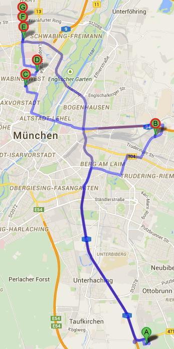
30 5 Evaluation of the Results With taking all listed arguments and constraints into consideration, we developed a program code in JAVA to calculate feasible solutions. First of all we want to present the calculated tours for the given example, which represents a sample day of LI- INITA s business. These tours are generated under the specified constraints and depict our solution for the original case of LIINITA s s business concept. Afterwards, variations of the setting and different conditions are presented and analyzed. Before evaluating the results, the input data of the example has to be defined. Starting from the IKEA facility located in Taufkirchen, near Munich, 276 customer requests within the city center of Munich have to be met. Those requests are equally divided into 138 pickup and 138 delivery requests. Pickup requests have an individual time window of 30 minutes, while delivery requests have a 20 minute time window of the desired departure time. The requests as well as the time windows are distributed from 9am until 8:40pm. Additionally, requests contain up to 3 customers which add up to a sum of 444 customers. Figure 5 shows a map of Munich with the correspondent 276 requests marked. Figure 5: Map with Example Customer Distribution in Munich; Microsoft Power Map for Excel 22

31 Due to the large amount of calculations needed, the longitude and latitude of every customers location is used to compute the linear distance between every request and is then saved into a distance matrix. This is done with the spherical law of cosines formula: arccos (sin (lat1 π π π π π ) sin (lat2 ) + cos (lat1 ) cos (lat2 ) cos (lon2 lon1 π )) R Since the longitude and latitude is given in degrees, the values have to be multiplied with π and divided by 180 in order to calculate the correct distance. The arccos() is multiplied by R = 6371 representing the earth s radius in meter. To apply the data to the code, the distance matrix is transformed into a time matrix. With the assumption of an average driving speed of 40 km/h every calculated distance is converted into a time, illustrating the travel time between all requests. The histogram of figure 6 displays the consistent frequency distribution of the time matrix data. An excerpt of the time matrix is shown in the appendix A. Figure 6: Histogram of Time Matrix Data Based on the time matrix and the specified constraints, as i.e. meeting the request s time window and starting a tour every 20 minutes, figure 7 gives an overview over the developed tours. 23

32 Maximum of 7 Vehicles needed 09:00 am 09:20 am 09:40 am 10:00 am 10:20 am 10:40 am 11:00 am 11:20 am 11:40 am 12:00 pm 12:20 pm 12:40 pm 01:00 pm 01:20 pm 01:40 pm 02:00 pm 02:20 pm 02:40 pm 03:00 pm 03:20 pm 03:40 pm 04:00 pm 04:20 pm 04:40 pm 05:00 pm 05:20 pm 05:40 pm 06:00 pm 06:20 pm 06:40 pm 07:00 pm 07:20 pm 07:40 pm 08:00 pm 08:20 pm 08:40 pm 09:00 pm 09:20 pm Gantt Chart, wohle day Re que st s in Cust ome r time [min] one t our: in one t our: Ti m e ( C o ## ## ## ## ## ## ## ## ## ## ## ## ## ## ## ## ## ## ## ## ## ## ## ## ## ## ## ,48 To u r 0 1: , ,48 To u r 0 2 : , ,63 To u r 0 3 : , ,04 To u r 0 4 : , ,94 To u r 0 5 : , ,79 To u r 0 6 : , ,6 To u r 0 7 : ,15 To u r 0 8 : , ,78 To u r 0 9 : ,02 To u r 10 : ,48 To u r 11: , ,53 To u r 12 : ,19 To u r 13 : ,29 To u r 14 : ,49 To u r 15 : ,24 To u r 16 : ,31 To u r 17 : ,5 To u r 18 : ,23 To u r 19 : ,63 To u r 2 0 : ,53 To u r 2 1: ,64 To u r 2 2 : ,82 To u r 2 3 : ,24 To u r 2 4 : ,62 To u r 2 5 : To u r 2 6 : , To u r 2 7 : , To u r 2 8 : , To u r 2 9 : , To u r 3 0 : , To u r 3 1: , To u r 3 2 : , To u r 3 3 : To u r 3 4 : , To u r 3 5 : , To u r 3 6 : , To u r 3 7 : , To u r 3 8 : ,71 Legend: 5 8 To u r 3 9 : , To u r 4 0 : , = Pickup; = Pickup&Delivery; = Delivery To u r 4 1: , To u r 4 2 : = Travel Time of a tour in Minutes (Rounded) , To u r 4 3 : = Start Time of a Tour in Minutes 646, To u r 4 4 : , ,48...= End Time of a Tour in Minutes To u r 4 5 : , To u r 4 6 : Tour 01: =Order in which Customers are visited , To u r 4 7 : , In this case: To u r 4 8 : Customer 2 is a."delivery Customer" , To u r 4 9 : Customers 1 and 3 are "Pickup Customers" To u r 5 0 : Quantity of currently needed vehicles: Figure 7: Solution Overview Numbe r of Numbe r of

33 All 276 requests with 444 customers are distributed in a total of 50 tours over the day, starting at time 0 in the code, which represents 9am. The beam chart depicts all tours according to their start and travel time and is divided into 3 variations: tours serving only pickup requests, tours with only delivery requests or tours with a combination of both. The figure shows tours with only pickup requests at the beginning and tours with only delivery requests mostly at the end of the day. The reason for this distribution are the opening times of IKEA. In the core time between 10:40am and 05:40pm are almost only combined PD tours as it is desired. The Gantt chart shows that the combined PD tours mostly begin with delivery request and afterwards serve pickup requests. An overview over the single trips can be seen in the appendix B. To calculate the presented solutions Euclidian distance between the requests was used. On the other hand the images of the tours in the appendix show the real route the vehicles have to drive. The tour based on Euclidian distance is depicted in an alphabetical order. Requests with a red circle represent delivery customers and requests without it represent pickup customers. Altogether the results look promising and efficient which can inter alia be seen at tour 28 (appendix B). At first the vehicle starts at IKEA with eight delivery customers. Those are brought back home before six pickup customers are gathered and drove back to IKEA. This tour is just one example out of many tours that in one trip serve more customers than the maximum capacity of the vehicle. But within the generated trips are also some single trips like tour twelve or 24, serving only one request. Here the TW of the pickup customer and the capacity of the vehicle limit the options of combining the request. Presumably there will be single trips throughout a day in LIINITA s business as a result of the constraining factors. A possible solution to avoid these single trips would be to adjust the customer request so that it fits to another tour. Although many resulting tours seem to be efficient, there are also tours that may need additional improvement. When taking a closer look at the tours, a few irregularities appear. It may happen that a tour passes by a customer, but instead of picking him up the tour visits other requests first before driving the way back again to the skipped customer (tour 32, appendix B). Due to the time windows irregularities like this may appear, but are correctly computed by the algorithms. Another reason for this may by the used Euclidean distance in the routing process. The application 25

34 on the daily business and therefore the use of more accurate distances could correct these irregularities and should for this reason be further examined. Over all 50 tours the average number of requests served per tour is 5.52 and the number of customers served is Those customers spend an average of minutes at a trip, while a vehicle needs ordinary minutes to drive one tour. All in all a maximum of seven vehicles are needed to meet every customer request in time. The allocation is nine single pickup tours, 16 single delivery tours and 25 tours combining pickup and delivery requests. Whereas the 2-Opt heuristic is able to improve 18 tours generated by the NN. A comparison of our calculated linear routes and the real driven routes according to their travel time showed an average deviation of around 20 minutes. Hence, in this example the linear routes are at an average 20 minutes faster than the real tours determined by the road network. An overview over the generated linear and real tours is presented in the appendix B. In the next step, various modifications to the time window constraint of pickup requests are made and evaluated. Therefore a waiting time is allowed, which represents the number of minutes the time window is violated. If for example a customer is picked up 5 minutes after his latest, desired pickup time, the waiting time is 5 minutes. To compare the results, alterations with different maximum waiting times 5, 10, 15, 20 and 30 minutes are made. Additionally the case of no time window restriction for the algorithms is evaluated. The reason for testing these different modifications is the assumption, that waiting time functions as an extension of the time windows. That on the other hand may result in more possible combinations and could improve the tour. Table 1 depicts calculated key values of the presented starting solution and of the TW modifications. 26

35 Table 1: Results of Waiting Time Modifications; Whole Day WT = 0 WT 5 WT 10 WT 15 WT 20 WT 30 No TW Constraint Total Amount of Tours: Total Amount of Vehicles needed: Average TravelTime of a Request: ,19 26,87 27,27 25,98 26,18 25,96 24,79 Average TravelTime of a Tour: 150,09 145,43 151,03 149,39 150,54 149,26 145,56 Average Number of Requests served per Tour: 5,52 5,41 5,75 5,75 5,75 5,75 5,87 Average Number of Customers served per Tour: 8,88 8,71 9,25 9,25 9,25 9,25 9,45 Average Driving Time of Vehicle: 62,96 62,13 63,92 65,09 65,29 64,89 63,76 Average WT of a Tour: 0 0,52 2,65 4,17 7,08 8,4 55,49 Average Sum WT of a Request: 0 0,1 0,46 0,73 1,23 1,46 9,45 Average Before- WT of a Request: Average After- WT of a Request: 0 0,03 0,25 0,46 0,59 0,89 8,19 0 0,06 0,22 0,26 0,64 0,57 1,26 Max WT: 0 4,9 9,85 14,55 19,81 28,9 86,89 Number of Only Pickup Tours: Number of Only Delivery Tours: Number of Combined Pickup and Delivery Tours: Number of improved Tours by TwoOpt: As it can be seen, in all cases of table 1 the amount of needed vehicles stays seven. The total amount of tours on the other hand decreases with a higher allowed WT. Just as the average travel time of a request shrinks from minutes of the starting solution to minutes with the removal of the time window constraint. 27

36 On the other hand the average number of requests and customer served per tour can be slightly increased by enabling waiting times. Of course the occurring waiting time average per tour accumulates with its limit. So the resulting maximum amount of WT for a request is always near the allowed limit. The allowance of a waiting time for pickup requests is accompanied by a decrease of the number of tours serving only pickup requests. This can be attributed to the wider TW, which provides a higher chance of combining pickup customer in PD tours. In contrast single delivery and combined tours may slightly vary but show no clear trend of de- or increase. Contrariwise, the number of tours improved by the 2-Opt shows a clear trend of progression. While 18 tours are improved with prohibited WT, an allowance of up to 30 minutes waiting time enables 23 improvements. The removal of the time window constraint increases this number even more to 30 improved tours. However this trend has to be deliberated and it should be measured to what extent it indicates improvement or not. The following chart illustrates a graphical overview over the presented data Waiting time Modifications Whole Day TW=0 WT=5 WT=10 WT=15 WT=20 WT=30 No TW Constraint Figure 8: Trend Chart for Waiting Time Modifications; Whole Day 28

37 Based on the evaluation of the used example the allowance of WT may generally improve the resulting tours. Less travel time and amount of needed tours to meet all requests can result in both customer satisfaction and economic gain. However, the disadvantage of this modification is the effort needed to handle waiting times at each customer request. A solution to this could be to propose a new pickup time to the customer according to his calculated waiting time. All in all the improvement has to be compared to the extra effort needed and based on that the conclusion has to be drawn, whether to allow WT or not. As the chart of figure 7 showed, the PD tours were concentrated in the time between 10:40am and 05:40pm, further referred to as the core time. Before and after that time no PD combination is possible, because of the opening hours of IKEA. The resulting single pickup and delivery tours are adulterating the data of the core time. To provide a better evaluation of the core time we separated its solution and measured its key data independently. The results can be seen in the following table 2 and are further compared to the solution before. 29

38 Table 2: Results of Waiting Time Modifications; Core Time WT = 0 WT 5 WT 10 WT 15 WT 20 WT 30 No TW Constraint Total Amount of Tours: Total Amount of Vehicles needed: Average TravelTime of a Request: Average TravelTime of a Tour Average Number of Requests served per Tour: Average Number of Customers served per Tour: Average Driving Time of Vehicle: ,53 27,43 26,6 26,21 26,26 26,34 25,49 185,34 184,68 185,27 182,55 183,79 185,27 182,04 6,73 6,73 6,97 6,97 7 7,03 7,14 10,93 10,93 11,31 11,31 11,38 11,41 11,54 69,34 68,56 71,52 73,45 73,48 73,77 72,35 Average WT of a Tour: 0 0,37 2,54 5,06 7,77 10,33 73,27 Average Sum WT of a Request: Average Before- WT of a Request: Average After- WT of a Request: 0 0,05 0,36 0,73 1,11 1,47 10,26 0 0,03 0,22 0,51 0,69 0,94 9,5 0 0,03 0,15 0,21 0,42 0,53 0,76 Max WT: 0 4,9 9,3 14,55 19,76 28,9 85,8 Number of Only Pickup Tours: Number of Only Delivery Tours: Number of Combined Pickup and Delivery Tours: Number of improved Tours by TwoOpt: Equally to the results of the whole-day-data, the total amount of tours decreases with increased allowed WT. About 30 tours are performed in the core time, which is 60% of all driven tours during the day. Since in the core time more requests are met in a tour than outside of it, the average travel time of a tour is in all evaluated 30

39 scenarios minutes higher than in table 1 before. An interesting fact that can be observed is that the average travel time of a request is not significantly higher than the one of a request calculated for the whole day. While the number of requests and customers served in a tour is increased in the core time the overall average driving time of a vehicle also rises. However, considering that for zero allowed WT around 2 customers are served more in a tour, an increase of 6 7 minutes driving time is tolerable. Although the waiting time data shows similarities to the data of table 1 it slightly decreased. This is an indication that the waiting time is more often caused by tours outside of the core time. Since in this scenario single delivery tours are not affected by the waiting time, single pickup tours are the cause for most of the waiting time. As already presumed over 80% of the tours in the core time are PD combinations. The trend of less pickup tours with higher waiting time can here also be observed. For the original case of zero waiting time allowed, around half of the tours can be improved by the 2-Opt. This number increases with a higher allowed waiting time, which can inter alia be seen in table 2 and the following chart figure 9. Waiting Time Modifications Core Time TW=0 WT=5 WT=10 WT=15 WT=20 WT=30 No WT Constraint Figure 9: Trend Chart of Waiting Time Modifications; Core Time 31

40 In sum, the evaluation of the core time data shows more accurate results than the complete set of data. While tours from the core time are longer and their average travel time is increased, the individual travel time does not suffer under it. The average travel time of a request stays under 30 minutes and is not significantly increased. Additionally, in the core time more customers are served in each tour, which is a sign of efficiency for the used PD combination. Nevertheless, the conclusion concerning the allowance of waiting times is here the same as before. The admission of waiting time has to be compared to the effort needed to manage it. If the decision would be to implement waiting time in the process, based on the evaluated data of the example we would recommend a maximum waiting time of 10 minutes. That is because on the one hand the tours start to show proper improvement in travel time, driving time and customers served per tour. On the other hand customer satisfaction should not be affected, when i.e. the customer is friendly asked to assimilate his pickup time for up to 10 minutes. Besides the modification of WT for pickup customers, we also evaluated different alterations for delivery requests. Therefore we switched the starting time of the tours and implemented a higher frequency of tours driven during the core time. The results of these modifications can be seen in the following table 3. Table 3: Results of Starting Time Modifications; Whole Day Starting Time: 0, 20, etc. Starting Time: 10, 30, etc. Starting Time: 5, 25, etc. 10 min frequency in core time Total Amount of Tours: Total Amount of Vehicles needed: Average TravelTime of a Request: 27,19 27,11 28,18 26,1 Average TravelTime of a Tour: 150,09 143,89 149,59 122,08 Average Number of Requests served per Tour: 5,52 5,31 5,31 4,68 Average Number of Customers served per Tour: 8,88 8,54 8,54 7,53 Average Driving Time of Vehicle: 62,96 62,6 63,13 59,73 Number of Only Pickup Tours: Number of Only Delivery Tours: Number of Combined Pickup and Delivery Tours: Number of improved Tours by TwoOpt:

41 The column with the starting time beginning at zero and continuing in a 20 minute frequency represents the starting solution. Compared to the two alterations where the tour starts ten or five minutes after the original starting time zero. The initial tour seems to be the better one at first sight. Less tours needed and in average more customers served per tour support that. However, starting the tours at the time of ten in the code enables the 2-Opt to improve eight more tours than in the starting solution. Moreover, in public transportation during rush hours an increased frequency is used to enhance the transportation service and customer satisfaction. Hence we implemented a ten minute frequency during the core time in the example. The results show a lower travel time and driving time as it was desired, but also more tours are needed. Even so many tours that an extra vehicle would be needed to meet all customer requests in time. As before we also evaluated these modifications for the core time, which can be seen in the following table 4. Table 4: Results of Starting Time Modifications; Core Time Starting Time: 0, 20, etc. Starting Time: 10, 30, etc. Starting Time: 5, 25, etc 10 min frequency in core time Total Amount of Tours: Total Amount of Vehicles needed: Average TravelTime of a Request: 27,53 27,19 28,88 26,03 Average TravelTime of a Tour: 185,34 177,63 183,89 134,83 Average Number of Requests served per Tour: 6,73 6,53 6,37 5,18 Average Number of Customers served per Tour: 10,93 10,63 10,37 8,41 Average Driving Time of Vehicle: 69,34 69,46 68,34 62,97 Number of Only Pickup Tours: Number of Only Delivery Tours: Number of Combined Pickup and Delivery Tours: Number of improved Tours by TwoOpt:

42 As in the core time from before, generally a higher travel time and longer driving time of the vehicle can be observed. Also more customers are served with each tour which is due to the higher concentration of PD combination during the core time. The evaluation of different starting types shows here the same trend as within the data of the whole day example. The starting time of ten followed by a 20 minute frequency is here also better in travelling time and improved tours by the 2-Opt. The increased frequency in the core time shows also the same trend as in the table before. Although lower travel time and driving time in average seem to be an improvement, the total amount of 15 single delivery tours does not prove efficiency. All in all different starting times may result in a better general solution, but this is dependent from the data used and therefore should be further analyzed before drawing a finite conclusion. Whereas the frequency of a vehicle starting at IKEA every 20 minutes proved to be feasible. An increased frequency of tours can improve customer satisfaction, but only if it is used for a short selected time span. A task for further studies could be a dynamic analysis of arriving customer requests and adjusting the tour frequency to it. 34

43 6 Conclusion In the previous chapter we presented the evaluation of the developed program code based on the given example. The comparison to different modifications showed feasible performance and practicability for LIINITA s business model. The goal for this study was to develop a suitable program code that can be used to generate valid solutions. Furthermore the variations analyzed in chapter 5 present an outline over possible improvements. Based on this studies evaluation, an allowed waiting time of ten minutes could enhance the computation efficiency. Before determining any concluding decision, this presumption should be accurately analyzed and could be the content of further studies. Moreover the implementation of a higher tour frequency may also result in an improved solution if it is applied in an exclusive time frame. To identify for which peak times it is feasible to use a higher tour frequency, also additional research is recommended before drawing a finite conclusion. All in all the compiled program constitutes a first acceptable solution for LIINITA s transportation needs while considering all required constraints. As incentive for further studies on this topic and to improve LIINITA s routing process it is also important to test other algorithms and heuristics. To generate a first starting solution it is possible to implement i.e. the Savings Algorithm or the SWEEP Method besides the NN. An alternative heuristic approach would be to use i.e. Simulated Annealing or Tabu Search instead of k-opt. Therefore a global optimum of the generated tours would be found and the results could be improved even more. Only with additional research on these modifications and a comparison to this study s results an optimal routing process can be guaranteed for LIINITA s business. 35

44 Reference List Biggs N. L., Lloyd E. Keith & Wilson Robin J. (1986): Graph Theory , Oxford Clarendon Press, p. 239 ff. Bundesministerium für Umwelt, Naturschutz und Reaktorsicherheit BMU (2012): Umweltbewusstsein in Deutschland 2012, p. 26 ff. Cordeau J.F., Gendrea M., Laporte G., Potvin J.Y., Semet F. (May 2002): A guide to vehicle routing heuristics. The Journal of the Operational Research Society, Vol. 53, No. 5, pp Croes G.A. (1958): A method for solving traveling salesman problems, Operations Research 6, pp Dantzig, George Bernard; Ramser, John Hubert (October 1959): The Truck Dispatching Problem, Management Science, Vol. 6, No. 1 (Oct., 1959), pp El-Ghazali Talbi; (May 2009): Metaheuristics: From Design to Implementation. John Wiley & Sons, Garey M.R., D.S. Johnson, L. Stockmeyer (February 1976): Some simplified NP-complete graph problems, Theoretical Computer Science, Volume 1, Issue 3, pp Hokey M. (September 1989): The multiple vehicle routing problem with simultaneous delivery and pick-up points, Transportation Research Part A: General, Volume 23, Issue 5, pp Laporte G.; Gendrea M.; Potvin J-Y.; Semet F. (September 2000): International Transactions in Operational Research, Volume 7, Issue 4-5, pp Lenstra J. K.; Rinnoy Kan A. H. G. (Summer 1981): Complexity of vehicle routing and scheduling problems, Networks Volume 11, Issue 2, pp

45 Mishalani Rabi G., Prem K. Goel, Ashley M. Westra, Andrew J. Landgraf (October 2014): Modeling the relationships among urban passenger travel carbon dioxide emissions, transportation demand and supply, population density, and proxy policy variables. Transportation Research Part D: Transport and Enviroment; Volume 33; pp Rajesh Matai, Surya Singh and Murari Lal Mittal (2010): Traveling Salesman Problem: an Overview of Applications, Formulations, and Solution Approaches, Traveling Salesman Problem, Theory and Applications, Prof. Donald Davendra, URL: problem-theory-and-applications/traveling-salesman-problem-an-overview-of-applicationsformulations-and-solution-approaches. Süddeutsche Zeitung (2014): Neue Mitte Möbelhaus im Hamburger Zentrum, published , URL: [Stand ]. United Nations World Commission on Environment and Development (1987): Our Common Future ("Brundtland Report"), Oxford, p. 41. Wang, X. & Regan, A.C. (2002): Local truckload pickup and delivery with hard time window constraints, Transportation Research Part B, Volume 36, pp

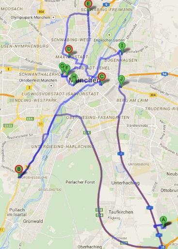
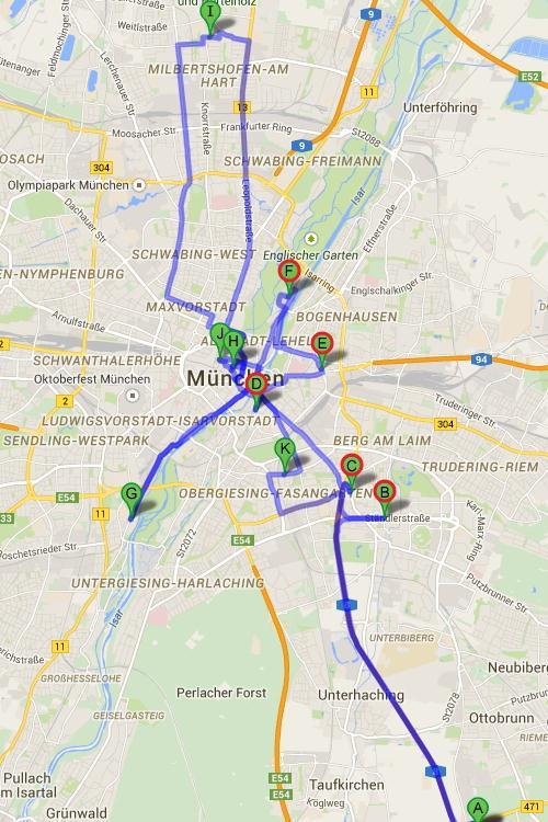
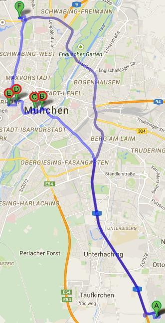
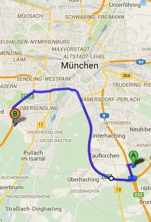
46 Appendices A. Excerpt of time matrix 38