Extensions and Applications of Land Use Transport Interaction (LUTI) Models Topic 1: Density, Accessibility, Retail Models

Transcription

1 Extensions and Applications of Land Use Transport Interaction (LUTI) Models Topic 1: Density, Accessibility, Retail Models Michael 8 July

2 Outline Spatial Interaction Ideas Again: Unconstrained Singly Constrained Models Modular Modelling: Coupled Spatial Interaction A Simple Example of Modularity: Lowry s Model DRAM-EMPAL Style Models Demand and Supply: Market Clearing Input-Output: The Echenique Models Integrated Large-Scale Model Structures Sketch for an Integrated Model Demonstrating an Aggregate Large Scale Model Very Rapid Prototyping of Aggregate Models

3 Spatial Interaction Ideas Again: Unconstrained Let me begin with spatial interaction models once again and first define key terms. We are going to divide our spatial systems into small zones like Census Tracts which can either be called origins or destinations. Origins are notated using the subscript i and destinations the subscript. Now the original gravity model can be stated as T PP PP i i K 2 2 d d KPP i 2 where we define T, P, P, d, and K as trips, populations, distance squared and a scaling constant i

4 In fact we can generalise the model first by noting that distance is like in the von Thunen model a measure of generalised travel cost c and the populations are defined as measures of mass or activity as origin and destination activities Oi, D Then Oi D Oi D T K KO id c c c Where is the so-called friction of distance parameter controlling the effect of generalised travel cost. When is large, the effect of distance is great and when it is small it is much less. This gives more trips when it is small than when it is big.

5 In all our models, we need to estimate these parameters and this is the process of calibration. We need to choose K and so that the predicted trips T are as close as possible to the observed trips obs T We can do this in this simplest of models by fitting a linear regression to the logarithmic version of the model and when we take logs we get T log log K logc O D i We find the parameters by minimising the sum of the squares (squared deviations) between the predicted obs 2 and observed trips, that is min min ( T T )

6 The original gravity model has been used for years but in the 1960s and 1970s various researchers cast it in a wider framework deriving the model by setting up a series of constraints on its form which showed how it might be solved generating consistent models. The constraints logic led to consistent accounting. The generative logic lead to analogies between utility and entropy maximising and opened a door that has not been much exploited to date between entropy, energy, urban form, physical morphology and economic structure. In particular the economic logic is called choice theory, specifically discrete choice theory

7 The key idea is to introduce constraints on the form that the model can take, and these relate to specifying what the model is able to predict. The more constraints we introduce on the model, the more we reduce the model s predictive power, but the idea of constraints also relates to what we know about the system in comparison with what we want to predict. The idea of a framework for consistent generation of a model is that we can then handle the constraints systematically as we will now show.

8 Singly Constrained Models We must move quite quickly now so let me introduce the basic constraints on spatial interaction and then state various models The constraints are usually specified as origin constraints and destination constraints as O i T D T i And we can take our basic gravity model and make it subect to either or both of these constraints or not at all

9 So what we get are four possible models Unconstrained T KO D i c Singly (Origin) Constrained so that the volume of trips at the origins is conserved Singly (Destination) Constrained so that the volume of trips at the destinations is conserved Doubly Constrained T trip volumes at origins + destinations are conserved The first three are location models, the last is the transportation model T A B O D i i AO D i c T i c B O D i c

10 Now the simplest way to work out what the constants mean is to note the constraint equations and then add and factor the model subect to the constraints. Let us show now the singly constrained gravity model which is T AO D c i i O i D c D c origin - constrained You can think of D c / D c as a probability of working in the origin and going to the destination. If we add up the trips in this equation over then we get O i --- this of course is the origin constraint

11 Now the singly constrained origin and then destination and the doubly constrained models follow directly and we will simply state their full forms noting that we need to find (1) (2) (3) T T T A i B AO i id c B O D c 1/ i A B O D c i 1/ i i B i D c AO c O i D D c D c O c i i O c origin - constrained destination constrained origin - destination constrained

12 Modular Modelling: Coupled Spatial Interaction So far we have ust singled out a module for one kind of interaction based on a variant of the gravity model - consider stringing these together as more than one kind of spatial interaction: Model 1 Model 2 Model 3.. Classically we might model flows from home to work and home to shop but there are many more and in this sense, we can use these as building blocks for wider models. This is for next time too What we will now do is illustrate how we might build such a structure taking a ourney to work model from Employment to Population and then to Shopping which we structure as --

13 First we have the ourney from work to home model as T P Ei And then the demand from home to shop And there is a potential link back to employment from the retail sector i F exp( c ), F exp( c ) T Wm exp( c m ) S m P, W exp( c ) S m S m m E m m m f ( S m ) T m S m E i P

14 A Simple Example of Modularity: Lowry s Model Lowry s (1964) model of Pittsburgh was a model of this nature but it also incorporated in it or rather its derivatives did more formally a generative sequence of starting with only a portion of employment basic and then generating the non-basic that came from this. This non-basic set up demand for more non-basic and so on until all the non-basic employment was generated, and this sequence followed the classic multiplier effect that is central to input-output models. A block diagram of the model follows

15

16 DRAM-EMPAL Style Models Essentially what we have here is the notion of simultaneous dependence i.e. one activity generates another but that other activity generates the first one what came first the chicken or the egg? Stephen Putman developed an integrated model to predict residential location DRAM and another to predict employment location EMPAL. In essence different models are used to do each the employment model tends to be based on very different factors it is a regression like model of key location factors not a flow model Now some models take the transport component out and use accessibility, then interfacing with a transport model that is built externally

17 Demand and Supply: Market Clearing So far most of these models have been articulated from the demand side they are models of travel demand and locational demand they say nothing about supply although we did introduce the notion that in simulating trips and assigning these to the network, we need to invoke supply. When demand and supply are in balance, then the usual signal of this is the price that is charged. In one sense the DRAM EMPAL model configures residential location as demand and employment location as supply but most models tend to treat supply as being relatively fixed, given, nonmodellable

18 However several models that couple more than one activity together treat supply as being balanced with demand, often starting with demand, seeing if demand is met, if not changing the basis of demand and so on until equilibrium is ascertained. Sometimes prices determines the signal of this balance. If demand is too high, price rises and demand falls until supply is met and vice versa. Often this is done simply to ensure demand is not greater than supply Most urban models do not attempt to model supply for supply side modelling is much harder and less subect to generalisable behaviour A strategy for ensuring balance is as follows for a model with two sectors like the one we illustrated earlier

19 In the following slide, we have two submodels first residential location and second retail location In each submodel, we first have interaction (trip distribution) and then location. The first loops in terms of interaction are for capacity constraints on supply, the second are for capacity constraints on location The second set of red loops involve reiterating the interaction and location so that we can get balance within the entire submodel The thick black loop in the middle couples the residential to the retail model, the thick black loop around the two models is used if retail predictions are to influence employment

20 Predict work to home trips Assign to network and check capacity Adust travel costs Predict population at home Check capacity Adust prices resid attractors Predict home to shop trips Assign to network and check capacity Adust travel costs Predict retail activity at shopping centres Check capacity Adust prices resid attractors

21 The decision to nest what loop inside what other loop is a big issue that makes these models non-unique If the supply side is modelled separately then the way this is incorporated further complicates the sequence of model operations. In the large scale integrated models that we will deal with next, these are crucial issues There is one further structural issue we will deal and this involves extending the models sectorally and the Echenique inputoutput formulation is a good example of this extension

22 Input-Output: The Echenique Models So far we have only developed couplings between models that are added together in ordered sequences that string sectors together apart from reference last time to the Lowry model which organised this sequence around the basic-non-basic employment multiplier. We can extend this to a series of linked causal multipliers between different sectors by extending this chain to an input-output model framework. In essence we define many different sectors involving households, labour, industries, services and so on and build the model so that there are consistent economic relations between each

23 Echenique s MEPLAN models are structured in this fashion. So too is the TRANUS model. We can introduce these as follows. Essentially the system is divided into production and consumption based on activities m that are produced in zone I, X im, and consumed as activities n in zone, Y n These are organised as in an input output table but noting that they are spatially specific X Y m i n i m n T T mn mn Here is the typical I-O table

24

25 The flows are based on spatial interaction models of the form T mn Y n m exp( c i m m exp( c ) m ) Where the generalised interaction costs also include other costs such as prices of good m at I c m p m i t m w m The order in which these equations are solved and linked together is given in the following flow chart Note that prices are determined from spatial interactions as m 1 m m p i logexp( c ) i

26 And then linked back to the prices of goods produced as p n m a mn p m a mn i Y T mn n The precise details of how the model works are extremely hard to figure out from the papers but the following flow chart goes some way to showing how the various elements are configured. This is a general point. In models that are coupled in this fashion integrated, then it is often hard to figure out the precise ordering or the structure. I am ust reading a PhD on the TRANUS model and this is a very complicated feature what is solved first the order.

27

28 Integrated Large-Scale Model Structures I will simply point you in the right directions here the Handbook I referred you to in the last lecture contains several very good papers on these issues and I will briefly present some notes from Miller s article

29 Here is a summary from his article of the key structure of such models and also their requirements

30

31 Sketch for an Integrated Model I am very quickly going to sketch an integrated model which builds on the ideas so far I will not disaggregate the model into m employment types and n housing types but we can assume that this is a complicating feature that simply makes the presentation trickier so we will simply deal with the aggregate version The model has three sectors employment, retailing and residential location with a link from retailing into part employment. Three different models are built for each sector spatial interaction for residential and retailing and a linear model of land development for employment

32 We begin with the residential, then retail sector, then trips capacities, and finally employment Residential location Retail location Capacitated Transport Constraints In the next slides, we show the loops which need to be invoked to balance demand and supply and to couple the submodels Employment location

33 We begin with the residential, then retail sector, then trips capacities, and finally employment

34 We begin with the residential, then retail sector, then trips capacities, and finally employment

35 We begin with the residential, then retail sector, then trips capacities, and finally employment

36 We begin with the residential, then retail sector, then trips capacities, and finally employment

37 We begin with the residential, then retail sector, then trips capacities, and finally employment

38 We begin with the residential, then retail sector, then trips capacities, and finally employment

39 We begin with the residential, then retail sector, then trips capacities, and finally employment

40 We begin with the residential, then retail sector, then trips capacities, and finally employment Residential location Retail location Capacitated Transport Constraints Here are all the loops Employment location

41 Integrated Urban Models Topic 2: Applications Michael 8 July

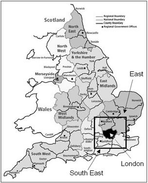
42 Demonstrating an Aggregate Large Scale Model We have broadened our residential location model for London to Greater London and the outer metropolitan area and we will demonstrate this in a moment Our current model is more disaggregate, more extensive and is really a suite of model types, it has an explicit money sector as house prices and wages are quite important We do not attempt to model markets this is quite impossible in London as the market hardly follows any known theory We simply use transport costs, wages and prices to determine residential location

43 Let me give you a quick summary of its structure: ORIGINS DESTINATIONS t = 1 ORIGINS Employment E i (t) T (t) DESTINATIONS S i (t) P (t) Population Economy Demography

44 Let me give you a quick summary of its structure: ORIGINS DESTINATIONS t = 1 ORIGINS Employment Wages and Revenues we i (t) i & v i T (t) d DESTINATIONS S i (t) d i P (t) p House Population prices Economy Demography Other flows, than people or money, materials and information?

45 To illustrate very briefly the sort of data that we have in the money sector that is driving this variant of the model and also the residential location equations And then we put wages, prices and transport costs together in the interaction model as follows

46

47 This is the order in which the operations take place Parameter Values Sequence of Model Functions Map Graphics Goodness of Fit Statistics: Deviations & r 2 Graphical Functions Activity Totals Logo Graph Data

48

49 I will run the model as it works very quickly on the desktop

50

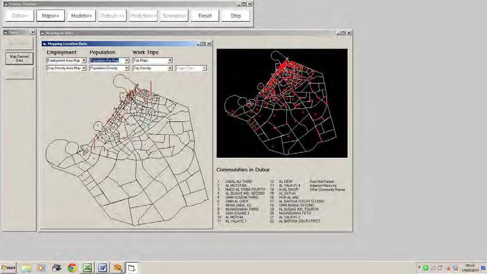
51 Applications Very Rapid Prototyping of Aggregate Models A New Retail Centre in Dubai

52 Where did we get the data in a data poor environment? Dubai Business Density derived from Google Places API Dubai Built-up area derived from Landsat 8 imagery Dubai Business Diversity Density Index

53

54

55

56

57

58

59

60

61

62

63

64 Applications A New Retail Centre in Dubai

65 Reading about integrated models is more tricky as these models are convoluted involved that clear statements are hard to find. Two papers are relevant. Iacono, M., Levinson, D., and El-Geneidy, A. (2008) Models of Transportation and Land Use Change: A Guide to the Territory, Journal of Planning Literature, 22, , and Hunt, J. D., Kriger, D. S. and Miller, E. J.(2005) Current Operational Urban Land- Use-Transport Modelling Frameworks: A Review, Transport Reviews, 25,

66 There is some good reading of all this material in Google Books in Button, K. J., Haynes, K. E., Stopher, P., and Hensher, D. A. (Editors) (2004) Handbook of Transport Geography and Spatial Systems, Volume 5 (Handbooks in Transport), Elsevier Science, New York