Trade Costs and Regional Productivity in Indian Manufacturing. Hanpil Moon

Transcription

1 Trade Costs and Regional Productivity in Indian Manufacturing Hanpil Moon Munisamy Gopinath Oregon State University

2 Overview Motivation for spatial and firmheterogeneity in responses to trade cost changes Theoretical basis from the heterogeneous firms model and new economic geography Empirical strategy relying on spatial econometrics and a time variant measure of trade costs Results from Indian manufacturing and their implications

3 Modeling Heterogeneous Firms Melitz (Econometrica 2003) ) Monopolistic competition model with an asymmetric equilibrium (Krugman s model is a special case) Introduces uncertainty on productivity prior to firm entry, subject to a fixed entry cost; plus a constant fraction of firms is subject to a death shock every period Equilibrium (price, quantity, revenue and profit) is summarized by the industry s average productivity level, which depends on cut off productivity Trade liberalization increases average productivity and changes the number of available varieties Higher average productivity implies higher welfare (holding variety gains constant)

4 Modeling Heterogeneous Firms (continued) Melitz and Ottaviano (RES 2008) Endogenous mark up (non CES utility function) and regional differences in market size Bernard et al. (AER 2003), Chaney (AER 2008), Baldwin and Okubo (JoEG 2006), Saito, Gopinath and Wu (CJE 2011) Empirical applications Helpman, Melitz andyeaple (AER 2004) extend the model to include FDI; Helpman, Melitz and Rubinstein (QJE 2008) identify heterogeneity and selection biases using aggregate data; Syverson (JPE 2004); Saito and Gopinath th(joeg EG2009)

5 Implications for Spatial/Firm Heterogeneity Industry: Moving from autarky to openness has asymmetric effects on firms within an industry (Melitz 2003) Low productivity firms exit (enter) Market share/resources reallocated to high productivity firms Spatial: Large markets additionally discipline firms via competition (Melitz and Ottaviano 2008) Productivity distribution is truncated from below Again, trade liberalization improves average industry productivity (mark up/self selection/sorting issues)

6 Focus on Average Industry Productivity We focus only on gains in average industry productivity and changes in cut off productivity Abstain from quantifying the variety gains from trade Feenstra (2008 CJE) and Broda and Weinstein (QJE 2006) ( ) ( ) are good examples for measuring variety based welfare gains

7 Equilibrium Distribution of Productivity For region r, industry k and time t: the equilibrium productivity distribution is truncated from below. The truncation point,, is determined by the zero cut off profit and free entry conditions Truncation increases with domestic and international competition (lower variable trade costs). Factor market explanation, e.g. increases in wages forces least productive firms to exit since mark up is constant (Melitz 2003) Product and factor market reasons (Melitz and Ottaviano 2008)

8 , Specifying Cut off and Average Productivity Cut off Productivity (left tail of the distribution) Inverse of equation (23) in Melitz and Ottaviano (RES 2008) International and domestic (variable) trade costs Average Productivity How about high productivity firms (right tail of the distribution)?

9 Empirical Strategy Objective here is to first identify regional productivity and attribute it to pure technical change (raw productivity) and agglomeration effects. Then, investigate the role of international competition and domestic infrastructure, i.e. changes in variable trade costs, on regional raw productivity distribution (mean, median, left and right tail). tail) Resource reallocation following changes in trade costs (future work).

10 Indian Manufacturing Significant trade reforms in Selected industries. Traditional (comparative) advantage in low tech, e.g. textiles Emerging advantages in electronics, pharmaceutical and transport industries Significant investments in infrastructure, especially since Significant spatial variations in income (per capita net domestic product ranges between $217 and $1932 among Indian states in 2006)

11 Industry Productivity Estimation Firm level production function: Two important differences from Levinsohn and Petrin s (2003) approach: U it and W it respectively denote urbanization economies and spatial spillovers (firm specific) W is a spatial weighting matrix commonly used in a spatial lag model

12 Estimation Issues Covariance between the spatial lag and error term In a spatial lag model, implies that shocks to one region s output spills over to other regions and hence, are correlated with the spatial lag of output Covariance between productivity and conventional input tlevels l (labor, capital) is non zero the usual suspect Covariance between agglomeration variables and productivity (self selection)

13 Production Function Data Centre for Monitoring Indian Economy (CMIE) Sample period: ; 8,472 firms Value of output and inputs available; appropriate deflators (in related literature) are used to identify quantities or constant rupee estimates: IV estimates for U it and W it y Location information has recently been included ( ) Urbanization economies is represented by output of all firms (manufacturing and services) withina three digit postal code area of a firm s location Spatial lag is given by output of firms in the same industry within a 50 km radius

14 Industry Definitions 1 Food 2 Textiles & Apparel 3 Wood, Paper & Printing 4 Chemicals & Rubber 5 Fuels & Mineral 6 Metals 7 Machinery 8 Electricals & Electronics 9 Transport Vehicles & Equipment (22 two digit NIC industries regrouped into the above 9 industries)

15

16 Firm Level Production Function Estimation Results: Dependent Variable is ln(y) Industry Wln(y) ue ln(k) ln(m) ln(l) ln(e) RTS Obs (a) ,180 (0.020) (0.003) (0.041) (0.008) (0.005) (0.004) (0.013) ,559 (0.008) (0.001) (0.009) (0.010) (0.004) (0.004) (0.009) (c) 2,997 (0.013) (0.001) (0.015) (0.026) (0.009) (0.006) (0.022) (a) , (0.018) (0.001) (0.020) (0.009) (0.003) (0.003) (0.010) (a) ,165 (0.010) (0.003) (0.026) (0.019) (0.009) (0.008) (0.019) (b) , (0.008) (0.001) (0.008) (0.007) (0.007) (0.005) (0.009) (b) ,320 (0.009) (0.001) (0.012) (0.009) (0.015) (0.006) (0.019) (a) ,403 (0.020) (0.001) (0.021) (0.016) (0.009) (0.006) (0.016) (a) ,858 (0.010) (0.001) (0.027) (0.014) (0.008) (0.005) (0.015) Note: Value in parenthesis is the bootstrapped standard error based on 200 iterations. All estimates are statistically significant at 1% level except (a) and (b) indicating statistically insignificance at 10% level, and significance at 5% level, respectively.

17 Estimated Raw TFP and Agglomeration Effects (AE), average Raw TFP AE Overall TFP Annual Growth Rate Industry Mean S.D. Mean S.D. Mean S.D. RTFP AE OTFP Total Industry Definitions: 1 Food; 2 Textiles & Apparel; 3 Wood, Paper & Printing; 4 Chemicals & Rubber; 5 Fuels & Mineral; 6 Metals; 7 Machinery; 8 Electricals & Electronics; 9 Transport Vehicles & Equipment

18 Now, What is a Region? Each state is considered to be a region: District level policy making is very limited Most observed policy differences are at the state level Data limitations: some of the infrastructure and natural endowments/amenities are not available on a time series basis at the district (or three digit postal code) level

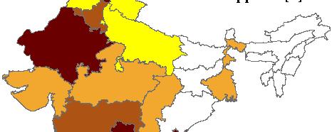
19 Textile Industry

20 Regional Raw Productivity Distribution For a given industry (k), mean, median and alternative percentiles of each region s (r) raw productivity at time t is specified as: Trade: international trade costs, Infra: Infrastructure (domestic trade costs) Choose 10% and 90% to avoid outliers (Syverson 2004) Some regions do not have enough firms (> 5) to derive distribution measures. So, the dependent variable can take zero values: tobit model

21 Trade Costs A number of problems with tariff data (bound versus applied, time variation, non tariff measures) We use a recent approach to measuring trade costs along the lines of Novy (2008), originally due to Anderson and van Wincoop (2003) and Head and Ries (2001). Accounts for both trade policy and geographic barriers (international transport costs) Measures trade costs as frictions in a gravity framework

22 Trade Costs, Continued trade flow in both directions intra country trade is the trade costs factor (one plus tariff equivalent) incurred form country c to India industry specific elasticity of substitution (estimated) Infrastructure is road length (surfaced and unsurfaced) divided by the total area of the state, i.e. ie road density (km/km square)

23 Industry Specific Trade Costs Industry Year AG(TC) AG(FT) ES Notes: AG (TC) and AG (FT) are average annual growth rate of trade costs and freeness of trade, respectively. ES is the estimate of elasticity of substitution for each industry. Industry Definitions: 1 Food; 2 Textiles & Apparel; 3 Wood, Paper & Printing; 4 Chemicals & Rubber; 5 Fuels & Mineral; 6 Metals; 7 Machinery; 8 Electricals & Electronics; 9 Transport Vehicles & Equipment.

24 Estimation Results of Tobit (Dependent Variable: Mean and Alternative Percentiles of Productivity Distribution) Percentiles 10th 50th 90th FT * *** (0.151) (0.233) (0.462) IN *** *** *** (0.030) (0.036) (0.072) SIN * *** (0.096) (0.115) (0.233) FTIN ** (0.007) (0.009) (0.018) FTSIN *** * (0.150) (0.182) (0.364) INSIN ** *** (0.027) (0.033) (0.066) HHI ** * (0.673) (1.261) (2.556) Pop. Share * *** *** (0.249) (0.301) (0.603) Pseudo R Log Likelihood Obs Censored Obs L.B F(6, 2247) F(8, 2247) Standard errors are in parentheses. ***, **, and * indicate significance at 1%, 5%, and 10% level, respectively. FT: Freeness of trade; Infra: Infrastructure; HHI: Herfindahl Hirschman Index; Pop. Share: Population Density.

25 Elasticities from the Tobit Model on Regional Productivity Distribution Percentiles 10th 50th 90th FT Elasticity *** *** (0.041) (0.053) (0.062) IN Elasticity *** *** *** (0.025) (0.023) (0.027) SIN Elasticity ** *** *** (0.021) (0.020) (0.023)

26 Estimation Results and Elasticities from the CLAD Model of Regional ProductivityDistribution Percentiles 10th 50th 90th FT * * * (0.141) (0.171) (0.364) IN *** *** *** (0.032) (0.033) (0.101) SIN ** ** (0.097) (0.122) (0.278) FTIN * (0.006) (0.008) (0.017) FTSIN * *** (0.161) (0.153) (0.429) INSIN ** * (0.025) (0.028) (0.083) HHI * (0.746) (1.372) (2.241) Pop. Share * * ** (0.291) (0.277) (0.460) Elasticity_FT Elasticity_IN Elasticity_SIN Pseudo R Obs Censored Obs L.B Notes: Numbers in parentheses are bootstrap standard errors with 200 draws. ***, **, and * indicate significance at 1%, 5%, and 10% level, respectively.

27 Trade Costs and Productivity Results Tobit versus CLAD models (homoskedastic and normally distributed disturbances) Freeness of trade (1/trade costs) CLAD model preferred Own infrastructure has the highest elasticity followed by that of the trade costs. Economic significance ifi Own infrastructure has contributed the most to raw productivity growth followed by that of the trade costs.

28 Spatial Differences in Elasticities: Textile Industry

29 Message After taking out the agglomeration/spatial spillovers, falling trade costs discipline firms (regardless of where they are) and improve industry productivity Infrastructureindependently and in concert with falling trade costs boosts productivity of firms It is tempting to interpret the larger effects of infrastructure on productivity as evidence of a more effective development strategy. However, knowledge on costs of each of these options is necessary in the search for efficient regional development strategies