Ricardo Model. Sino-American Trade and Economic Conflict

Transcription

1 1 of 18 6/10/2011 4:35 PM Sino-American Trade and Economic Conflict By Ralph E. Gomory and William J. Baumol March 22, 2011 In this note we look carefully at the impact on a developed nation of the economic development of its trading partner; a trading partner that is developing from a rather undeveloped state. If you want to keep the China-U.S. relationship and the impact on the United States of China s development in mind as a possible example, you will not go far wrong. We will discuss what a very standard model, the Ricardo model, shows about this situation. We will see that this very familiar model, properly analyzed, has a number of very unfamiliar consequences. Notably: The economic development of your trading partner can be harmful to you, the home country. Although the effect of that development starts out good, it ends badly. That there is a dominant and dominated relation possible between the two countries that is good for the dominant one and bad for the dominated one. A country can attain a dominant position only by having an undeveloped trading partner. This can occur naturally if the trading partner is simply there in an underdeveloped state, or the underdevelopment can be brought about by mercantilist actions that destroy that partner s industries. There is inherent conflict not only between a nation in a dominant position and its trading partner, but also between that dominant nation and what may loosely be called the interests of the world. In a two-country model of the sort we discuss here this simply is measured as the sum of the benefits obtained by the two countries economies. We assert that from a world point of view, having either nation dominant is bad. While a country cannot gain a dominant position solely by building up its industries, it can avoid a dominated position by developing its own industries and not allowing them to be destroyed. We will explain more clearly what we mean by these assertions as we go along... We will also explain enough about the Ricardo model to make that intelligible to those not already familiar with it. Ricardo Model This model, or at least pieces of it, has been taught to generations of students, and much of what is taught did not originate with Ricardo. It has been, and still is, enormously influential. (A good reference for this is Krugman and Ostfeld, International Economics, Theory and Policy, Chapter 8). Figures 1 and 2 (Appendix D) briefly describe the inputs to the Ricardo model and also what comes out of it. For those more deeply interested, the actual equations of the model and an explanation of them are attached as Appendix A. What the model does for you is this: You enter certain values, like the level of productivity, in various industries and the scale of the demand for the goods, the size of the labor force, etc. into the model (Figure 1). The model then computes the economic outcome, the result of trade between the nations you have described (Figure 3). For example, it computes which country produces how much of what products, what prices are, and also what products and product quantities the nations get to consume. However in this note we want to emphasize not the model itself, but the change in the economic results that come out of this very standard model, as we allow the nations to develop, i.e., increase, their productivities. The Ricardo Model itself is static, one set of inputs, one set of outputs. But we can use it to look at change by giving it a series of different inputs and looking at the different outputs that result.

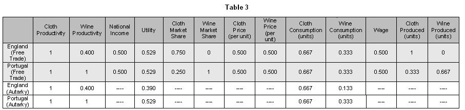
2 2 of 18 6/10/2011 4:35 PM The Simplest Model and Bar Charts We will start our discussion with a two-good model, the famous England-Portugal, wine-cloth model. But we will explore the results of the model not for just one set of inputs, but for several. Initially the inputs will reflect the improvement in the productivities of England s trading partner, Portugal. The model will allow us to explore the impact of Portugal s improvement on both countries. On this subject, the impact of your trading partner s development, there is a widespread belief, especially among those who have been exposed to the theory of comparative advantage, that improved productivity in your trading partner is not only good for your developing trading partner but also for you, the home country, as well. Although this belief is widespread, there is little basis for it in the economic literature. In fact, just to mention two famous names, Professor Hicks in his 1950 inaugural address and Paul Samuelson in a 2006 paper clearly state that the improvement of your trading partner s productivity can be harmful to you the home country. Not to mention the 2001 Gomory-Baumol book Global Trade and Conflicting National Interests in which this effect was the major topic. Nevertheless, the possibility that the model can show harm to the home country from the development of its trading partner, is almost never discussed. And the thought that in the real world the development of China might be bad for the United States is, in our experience, pretty unmentionable. An Example We now get ready to look at one example. In our discussion, we choose the unit of production so that the technological limit is expressed as a productivity of 1. For example, if the best possible output from cloth production is 2 rolls of cloth per worker per day, we choose two rolls as the unit of production, and producing two rolls is said to have a productivity level equal to 1. Producing, half as much, one roll a day, then is taken to give you a productivity of 0.5. At the start (Figure 3), Portugal is good at wine, productivity 1; England is good at cloth, productivity 1. Both are not nearly as productive in the other good. England is poor at wine, productivity 0.4, and Portugal is poor at making cloth, productivity 0.4. In addition to the productivities, the demand structure matters too. In our example both countries want to spend 2/3 of their income on cloth and only 1/3 on wine. Appendix D has a series of bar graphs showing the effect of Portugal improving its cloth productivity. Figure 4 and Figure 5 show the cloth and wine consumption of the two countries at the beginning, then after Portugal s cloth productivity improves from 0.4 to 0.7 and then after it improves further to 1.0. At the beginning we have a situation in which England makes all the cloth and Portugal makes all the wine. This is a good situation for England because England makes so much of what people want. The demand for cloth is assumed here (for illustration) to be twice as great as the demand for wine. Essentially England has the productive industry and Portugal has the unproductive one. The Portuguese are working at a low wage and 2/3 of what they make goes to be consumed in England. This is a good dominant position for England, and a poor position for Portugal. England s consumption of both cloth and wine is twice that of Portugal. a However, the Portuguese understand that too and they start to increase their productivity in textiles and get into making cloth. The second bar graph in Figure 6 shows immediately that the improvement in Portuguese cloth making is good for Portugal; it is good for Portugal even though Portugal s productivity, at 0.7, is still below England s 1.0. The second bar graph in Figure 7 also shows that this change has hurt England. b

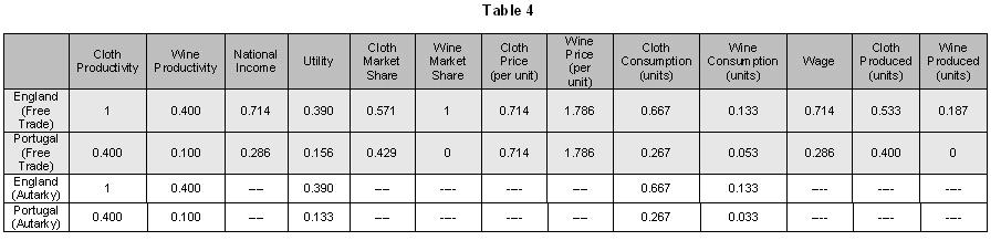
3 3 of 18 6/10/2011 4:35 PM When Portugal improves its cloth productivity to 1.0, matching England, the story is the same, only more so, with even bigger gains for Portugal. c Portugal improves its consumption of cloth at each step and its income and its utility both go up. England still makes only cloth but it now divides the cloth market with Portugal. Its share of world production has gone down, its share of world income has gone down, its exchange rate with Portugal has worsened, and it therefore gets less wine for its money than before. So at each step, England s wine consumption decreases while its cloth consumption holds stable. Meanwhile, it s all good for Portugal. Portugal s consumption improves at every step. What is going on? We will see below that this example is typical; it is common for the improvement in your trading partner to be harmful to the home country. But the idea that your partner s economic progress is always bad for you is not correct either. Let us extend out example. In this next example we start Portugal s development at an even lower state. Instead of Portugal initial productivities being (Cloth, Wine) = (0.4, 1.0) we will start Portugal s wine productivity at 0.1 and let it increase to 0.6 before arriving at the 1.0 which was Portugal s starting productivity in wine in our earlier example. Throughout we keep England s productivities fixed at (Cloth, Wine) = (1.0, 0.4) At our new starting position England s comparative advantage is in wine. It is the sole producer of wine and it divides the cloth market with Portugal. Although it is the sole producer of wine, it is nevertheless not very productive in wine, so its wine consumption is low. Its cloth consumption remains fixed at its autarky value, that is, the state at which it imports no cloth but produces it all at home. d As Portugal increases its wine productivity to 0.6 e and then to 1.0 we see that England s wine consumption goes steadily up while its cloth consumption is stable (Figure 6). Figure 7 shows us that Portugal first improves its consumption of both cloth and wine, and then at the second step it has a further gain in cloth consumption. Portugal s improved productivities have helped both countries. What we will see later in this note is that this example is typical. Generally if your trading partner moves from a very undeveloped to a more developed state, the effect on the home country is good. However after a rather early stage of development the effect changes and becomes bad for the home country. As we said in the introduction, the development of your trading partner starts out good but ends up being bad for you. Where we are going? We will next move beyond a single example. In fact we are we are going to go beyond one or two or three equilibrium examples and look instead at the pattern formed by all possible equilibria. That means that we will consider all productivities equal or less than 1. But to do this we have to shift gears and have a way to look at many outcomes in a way that will permit us to see the outcomes from many examples at the same time. The Utility-Income Diagram In our bar charts so far, we have seen the actual outputs in wine and cloth and also two summary terms, utility and income. Income tells you how what fraction of world value at current prices is created or consumed by a country, and utility is a measure of how satisfying the goods bought with that income were for the country s consumers. Throughout we use the standard Cobb-Douglas utility, which weights the quantities of goods consumed by the demands for them. f

4 4 of 18 6/10/2011 4:35 PM With a two good model just looking at the two goods usually tells you unambiguously which of two equilibrium outcomes is better without needing utility or an equivalent. But once you have more than two goods some measure like utility is definitely needed. When we reach the part of the note where we deal with more than two goods we will discuss this further and indicate why our results are relatively insensitive to the choice of measure. We will use Income and Utility to display the economic outcomes as points in an Income/Utility diagram (Figure 8). Income, or rather share of world income, is horizontal, utility is vertical. Up is goodness in this chart; points that are higher up have more utility and are better. To display the equilibrium result takes a pair of points. The height of the black point measures England s utility and its horizontal distance from the zero on the right its share of income. The gray dot s height shows Portugal s utility, and as the two shares add up to 1, its distance from the 1 on the horizontal scale measures its share of income. Up for a point is always good. Moving left to right increases England s share of world income, moving right to left increases Portugal s. Figure 9 has the five equilibrium points we calculated before. See how (moving from right to left) the points for Portugal go steadily up, meaning more utility and a better outcome for Portugal. But see also how those for England first go up and then go down. g An Important Observation We could also interpret the points in a different way. Let us take them in reverse order. We could start with Portugal having a productivity of 1 in cloth; then, as we move from left to right, Portugal s cloth productivity would go down step by step. Our diagram would clearly tell us that, for a while, Portugal s loss of productivity would help England. It would also tell us that if the Portuguese loss of productivity goes too far, then it starts to hurt England. Once you become aware of the possibility, in this standard model, that a country s loss can be its partner s gain, we also have to consider the possibility that perhaps in the real world, too, a country can gain from another s loss. Perhaps China can gain from losses in U.S. productivity. Moving toward the Basic Pattern Let s add a few more points to the picture. Ricardo s example in fact had Portugal more productive in both cloth and wine than England. But let s be generous; we will try out all sorts of different productivities. h Each gives us two points in the diagram (Figure 12). Higher points are good in this diagram; high points give a country more goods, especially the goods it wants. Points on the right are those in which country 1 (England) has a large share of world income. Those on the left give Portugal (Country 2) a large share. The Basic Two-Good Pattern If you look hard at Figure 10, you can see that the upper edge of the region where the points lie has a vague sort of shape. It is clearer if you look first at the highest black points and where they lie, and then at the highest gray ones. It is possible by mathematical analysis to short-circuit the tedious process of finding one new equilibrium point at a time. i There is an underlying pattern that emerges. Here it is: Figure 11. Note that all the black dots outcomes for country 1, England lie under the blue curve. All gray dots lie under the red curve. What the mathematical analysis shows is that if we were to compute all possible equilibria, all the space under the

5 5 of 18 6/10/2011 4:35 PM blue curve would be solidly filled with black dots and all the space under the red curve would be solidly filled with gray dots. Dots lying on or near these upper boundary curves are the highest and give the best outcomes. For any equilibrium dot below the boundary there is a boundary equilibrium that gives more to both countries. Our five examples from the bar charts are all on the boundary. Examining some Special Points It is clear that the starting point of our first example, located at the peak of the blue curve is the best possible for England (highest point), and that it is very poor for Portugal. At this point England makes all of the most desired good, cloth, at a high wage, and the entire Portuguese nation is devoted to the less desired good, wine, and receives a low wage. This arrangement is good for England and bad for Portugal. Since we are considering all possible productivities, we should also consider the point where Portugal is good at cloth and England good at wine with the productivities interchanged... That is the peak of the red curve. This is a good outcome for Portugal and a poor one for England. This is the point where Portugal would want to be. Remark: Two significant dominant points exist, an England dominant point and a Portugal dominant point. Each point produces 2/3 income for one, and 1/3 for the other. Each country strongly prefers this dominant outcome to someplace in the middle where each produces half the value of the world s goods. In the middle, between these two possibilities, is an equilibrium that is a compromise. In the two- good model we have been discussing, it is the equilibrium where England and Portugal divide the Cloth market, with England having the larger share,, and Portugal makes all the wine. j It is a very important outcome of our analysis that from the middle point a country cannot go to its dominant point without lowering the productivity of the trading partner. If Portugal cannot lower England s productivity in cloth, it cannot get from the middle to its best point. We will say more about the middle point as part of our discussion of the World Boundary Curve and larger models. World Utility, World Boundary Curve, and Three Important Points We can measure world utility, in this two country world in the same way as we measured national utility.- Essentially, you measure the outcome as if the two countries were one country, and give that combined country all the goods produced by the two countries. We measure the world output using the utility function of one or the other country. In this case, as we have the same demand structure, it does not make a difference which we choose. Each equilibrium then gives us a world utility dot in addition to the England and Portugal utility dots we have already. All these world utility dots lie under the World Boundary Curve which we see in Figure 12. In Figure 13, we mark the highest points on the England and Portugal and World Boundary curves. An important conclusion: Each country prefers to be dominant, with a dominated trading partner. The world however prefers something in the middle. There are therefore three special equilibria: the one that is best for England, the one that is best for Portugal, the one that is best for the world. Larger models At this point we should ask, Is this something special about the two-good model, or is this pattern one that persists as we add more and more different goods? The mathematical analysis shows the pattern persists.

6 We show here examples of a six-good model (Figure 14) and an 11 good model (Figure 15). In these models we also allowed the two countries to have different possible largest productivities. The largest possible values of the productivities of the two countries in these examples were not all 1. This enables us to discuss situations in which the countries have inherent productivity limitations; after all if they have no oil under their countries they cannot obtain a productivity of 1 in oil no matter how hard they try. Although less important than in Ricardo s time, countries still have inherent productivity differences. The data for these two models is given in Appendix C. The main difference that comes with size is that the lumpiness disappears, but more importantly the peak of the world curve is much higher relative to the dominant points associated with England or Portugal. Total world output and consumption suffers at these dominant points relative to the world maximum, because of the loss of productivity necessary to get to either one of the two dominant points. We see these effects in larger models, whether they are six-good, or eleven-good, or even larger. Note that in Figure 15 there is a limiting shape that usually starts to become clear with about 8 or more goods. The boundary curves approach the limiting curves as the number of goods increases. k In that shape we can see that as the red boundary curve lifts off from 0 and moves right, the blue curve goes up too. But after passing that dominant point, the blue trends steadily down. We see that there is an early phase where the red curve s rise benefits both countries, but after passing that dominant point the effect of red s further development is uniformly bad for blue. The effect of development starts good, but ends bad. Note that in our large examples, and this is what occurs in almost all examples, the world maximum occurs in the middle, far from either the England Dominant or the Portugal Dominant positions. l The remark we made in the two-good case, that from the middle point a country cannot go to its dominant point without lowering the productivity of the trading partner, generalizes to larger models. The statement for many-good models is this: Find the equilibrium that results when both countries are fully developed. Then: (1) Neither Country can get a better equilibrium without lowering the productivity of its trading partner in one of the industries in which the trading partner has positive market share at the classical equilibrium (2) Neither Country need accept a worse equilibrium unless it loses productivity on one of the industries in which it has a positive market share at the classical equilibrium. Summary In a world in which countries can learn and change their productivities, many things can happen that were really not possible in Ricardo s time. We have used the Ricardo Model to reflect this new world. In a world in which productivities are often not fixed by nature but are often acquired we have shown the following possibilities: That the economic development of a trading partner can be harmful to the home country.although the effect of that development starts good, it ends badly. That there is a dominant and dominated relation possible between two countries, a relation that is good for the dominant one and bad for the dominated one. That a country can attain a dominant position only by having an undeveloped trading partner. This can occur naturally if the trading partner is simply there in an underdeveloped state, or the underdevelopment can be brought about by mercantilist actions that destroy industries. There is inherent conflict not only between a nation in a dominant position but between that dominant partner and the interests of a two-county world. While a country cannot gain a dominant position by building up its industries, it can avoid a dominated position and assure a good outcome by developing a particular subset of its own industries and not allowing them to be destroyed. 6 of 18 6/10/2011 4:35 PM

7 7 of 18 6/10/2011 4:35 PM It is possible that the United States and China were in the dominant and dominated position some time ago. We should recognize that China s evolution away from that state can be harmful to the United States. Furthermore we can observe that China s gain has been accompanied by the disappearance or at least decline of a number of our industries. We need to be cautious because, as these standard models show, there is a distinct possibility that this situation can even lead to significant loss through deindustrialization in an initially prosperous economy. Let us make sure that we do not allow our industries to be destroyed so that we become a dominated nation. This very standard model suggests that such an outcome would be both disastrous for the U.S. and bad for the world. *You can try out various inputs or play with the Ricardo model by using our interactive spreadsheet. Notes a More detail on this outcome is given in Table 1, Appendix B b More detail on this outcome is given in Table 2, Appendix B c More detail on this outcome is given in Table 3, Appendix B d More detail on this outcome is given in Table 4, Appendix B e More detail on this outcome is given in Table 5, Appendix B f If a country consumes a quantity qi of the ith good and its demand for that good is d i then the Cobb-Douglas utility obtained d1 dn by the country is the product q 1 qn g The height of the black dot at each equilibrium is obtained by taking the Cobb- Douglas utility for Country 1 and dividing it by the Cobb-Douglas utility obtained with no trade (autarky) but with Country 1 fully developed, ( all productivities =1). This means that for Country 1 we are taking as the unit of utility the best Country 1 could attain alone, without any imports. That height is marked with a 1 on the U1 vertical scale. We do the same for Country 2, the height of each grey dot is measured against the 1 on the U2 vertical axis which is the best Country 2 can do without trade. h The simple spreadsheet calculation used to compute each equilibrium is attached with an explanation of how to use it. This enables our readers to produce equilibria with productivities and demands of their own choosing. i The methods required for this come from the area of integer programming, a subject one of us (Gomory) pioneered some fifty years ago. j Table 3, Appendix B k The limiting curves are discussed in detail in Reference 4. Furthermore, for each Z 1 value it can be shown that there is a finite list of equilibria that dominate the rest. For every equilibrium not on that finite list there is an equilibrium in the list that produces as much or more of every good. In addition all these strong equilibria lie close to the boundary curves. If we were to choose a different way to measure outcomes, that would produce new boundary curves, but those boundary curves could only pass through members of this list and can therefore not look very different from those we have now. l The world maximum is closely associated with what in our earlier papers we call the classical equilibrium. This is the equilibrium obtained when both countries have obtained their maximal productivities. For example in the example 6 good model, the classical equilibrium assigns three industries in the order of their comparative advantage to England, the remaining three to Portugal. When demands are the same in both countries the World Boundary Maximum is directly above the classical equilibrium.

8 8 of 18 6/10/2011 4:35 PM References 1. "A Ricardo Model with Economies of Scale," Ralph E. G omory, Journal of Economic Theory, April 1994, Volume 62, No. 2, pp "A Linear Ricardo Model With Varying Parameters," Ralph E. Gomory and William J. Baumol, Proceedings of the National Academy of Sciences, U.S.A., 1995, Vol. 92, pp "Analysis of Linear Trade Models and Relation to Scale Economies, " Ralph E. Gomory and William J. Baumol, " Proceedings of the National Academy of Sciences, U.S.A., 1997, Vol. 94, pp National Trade Conflicts Caused by Productivity Changes: The Analysis With Full Proofs," Ralph E. Gomory and William J. Baumol, C. V. Starr Economic Research Report (New York University), November 1998, RR # Global Trade and Conflicting National Interests, Book, Ralph E. Gomory and William J. Baumol MIT Press, Cambridge, MA, Globalization: Country and company interests in conflict. Gomory, R., & Baumol, W J. Journal of Policy Modeling (2009). 7. "Trade, Education, and Innovation: Prospects for the U.S. Economy Ralph E. Gomory and William J. Baumol, Journal of Policy Modeling (to appear). Appendix A: Equilibrium Equations Notation In our standard Ricardian model there are two countries and n industries. The quantity q i, j of good i produced in Country j is determined by linear production function e i, j l i, j with l. i, j denoting the amount of labor employed in Country j in producing good i. The size of labor force for each country is L j. Country j s consumption of good i is denoted by y i, j and its production of good i by q i, j. Country j s productionshare or market share of world output of good i is represented by x i, j = q i, j / (q i, 1 +q i, 2 ), so that the vector x = (x i, j ) describes the pattern of production. Each of the two countries participating in trade has a given utility function of Cobb-Douglas form with demand parameters d i, j. The price of good i, p i, and w j, the wage in Country j, and Y j the national income of Country j. are all expressed in monetary units. The standard equilibrium equations given below are homogenous in these variables. This means that if we choose a different monetary unit thus replacing any set of p i, w j, and Y j values at an equilibrium by kp i, kw j, and ky j, these values too would satisfy the equilibrium conditions while leaving all the non-pecuniary variables such as q i, j andl. i, j unchanged. We eliminate this ambiguity by choosing at each equilibrium the monetary unit, the MU, that that makes the total world income Y 1 +Y 2 = 1 MU. The national incomes with this normalization we will refer to as Z 1 and Z 2. We will then have at each equilibrium uniquely determined pecuniary values and the uniquely determined national income, expressed in MU units, satisfy Z 1 +Z 2 =1. Equilibrium Conditions For any given vector of productivity parameters e= {e i, j } there is a stable equilibrium giving a national income Z j and a utility U j for each country.

9 9 of 18 6/10/2011 4:35 PM The first equilibrium condition stares that national income or consumption Z j in Country j must equal the total value of the goods produced in Country j.. With a Cobb-Douglas utility each country spends d i, j Z j on good i, so total world expenditure on the ith good is (d i,1 Z 1 +d i,2 Z 2 ). Since the fraction produced in each country is x i,j the balance of the value of production and consumption requires for each country: (1.1) Second, we have a zero-profit condition. World expenditure on Country j's output of good i all goes into the wages of the labor l i, j employed in that industry, so: (1.2) Third, is the full-employment requirement for each country: This is expressed as the condition that the wage rate times the country's total labor force equals national income:(the wage rate condition): (1.3) Fourth, we have the requirement that, for each good the value of the output of good i at the equilibrium price p i equals the total amount consumers are willing to spend on it: (1.4) Where the second form of (1.4) follows directly from the first by multiplying through by x i, j = q i,j /(q i,1 +q i,2) and using (1.2). Finally, we have the conditions that require that in each industry production, or equivalently market share, is always assigned to the producer or producers with the lowest unit cost. For example, if in industry i, w 1 /e i,1 < w 2 /e i,2, then x i, 1 =1 and x i, 2 = 0. More generally: (1.5) It is of course the actual producer s unit cost that determines the price p i. The conditions (1.5) include the familiar comparative-advantage criterion. Note that because of (1.1) the equilibrium conditions include balanced trade.

10 10 of 18 6/10/2011 4:35 PM Appendix B

11 11 of 18 6/10/2011 4:35 PM Appendix C Data used for the six good model Labor force sizes: L[1]=L[2]=1 Maximum Possible Productivities: e[1]={1,1,1,1,0.7,0.5}, e[2]={0.5,0.7,1,1,1,1}. In four of the six industries one country or the other is limited in its productivity. This could represent, for example, the absence of natural gas or oil or some other natural resource. The third and fourth industries are industries in which a high level of output is attainable for both countries. Demands: d[]1=d[2]= (1/6,1/6,1/6,1/6,1/6,1/6}. There is an equal demand for all six industries. Eleven Good Model In contrast to the six good model, in this eleven good model the numbers both for the maximum possible productivities and for the demands have no particular structure. Country 1 Maximum Productivities: e[1]={0.97, 0.92, 0.72, 0.94, 0.84, 0.52, 0.73, 0.77, 0.53, 0.91, 0.89} Country 2 Maximum Productivities: e[2]={0.52, 0.61, 0.91, 0.92, 0.84, 0.97, 0.83, 0.92, 0.31, 0.83, 0.72} Country 1 demand: d[1] = {0.033, 0.140, 0.073, 0.100, 0.153, 0.046, 0.053, 0.066, 0.133, 0.086, 0.113} Country 2 demand: d[2] = {0.080, 0.806, 0.169, 0.112, 0.177, 0.032, 0.048, 0.104, 0.056, 0.096, 0.040} Additional note: This is also the first example in which the two countries have different demand structures. If you look closely at Figure 15 you will see that the world boundary does not come down exactly to the unit level of the U2 vertical axis. This is because we are using the utility function of Country 1 to measure the value of total world output. When this measure is applied to Country 1 output alone, which is what we see on the extreme right of the diagram, it should come out as 1 which it does. But when applied to the Country 2 output alone, as it is on the extreme left (Country 2 share = 1) there is no reason for it to produce the 1 which is what the Country 2 utility function would produce. Appendix D Figure 1

12 12 of 18 6/10/2011 4:35 PM Figure 2 Figure 3

13 13 of 18 6/10/2011 4:35 PM Figure 4 Figure 5

14 14 of 18 6/10/2011 4:35 PM Figure 6 Figure 7

15 15 of 18 6/10/2011 4:35 PM Figure 8 Figure 9

16 16 of 18 6/10/2011 4:35 PM Figure 10 Figure 11

17 17 of 18 6/10/2011 4:35 PM Figure 12 Figure 13 Figure 14

18 18 of 18 6/10/2011 4:35 PM Figure 15 Issues: Economic Growth The New America Foundation 1899 L Street, N.W., Suite 400, Washington, DC th Street, Suite 901, Sacramento, CA Additional Contact Info New America is a registered trademark of the New America Foundation.