Queuing Theory. Carles Sitompul

Transcription

1 Queuing Theory Carles Sitompul

2 Syllables Some queuing terminology (22.1) Modeling arrival and service processes (22.2) Birth-Death processes (22.3) M/M/1/GD/ / queuing system and queuing optimization model (22.4) M/M/1/GD/c/ queuing system (22.5) M/M/s/GD/ / queuing system (22.6) M/G/ /GD/ / and GI/G/ /GD/ / models (22.7) M/G/1/GD/ / queuing system (22.8) Finite source models (22.9) Exponential Queues in series and open queuing networks (22.10) M/G/s/GD/s/ system (BCC) (22.11) *Chapter 20. 4th edition

3 Some queuing terminology

4

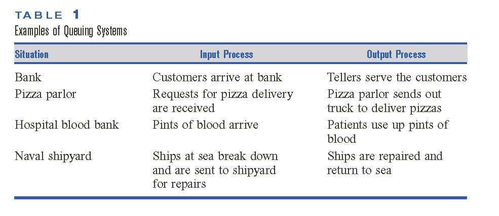
5 Input process The input process is usually called the arrival process. Arrivals are called customers. We assume that no more than one arrival can occur at a given instant. For a case like a restaurant, this is a very unrealistic assumption. If more than one arrival can occur at a given instant, we say that bulk arrivals are allowed. We assume that the arrival process is unaffected by the number of customers present in the system. The arrival process may depend on the number of customers present: when arrivals are drawn from a small population (finite source) when the rate at which customers arrive at the facility decreases when the facility becomes too crowded (the customer has balked).

6

7 Output process The output process is often called the service process. We usually specify a probability distribution - the service time distribution - which governs a customer s service time. We assume that the service time distribution is independent of the number of customers present. We study two arrangements of servers: servers in parallel and servers in series

8 Queue discipline The queue discipline describes the method used to determine the order in which customers are served. FCFS = First come first serve LCFS = Last come first serve SIRO = Service in random order Priority queuing discipline classifies each arrival into one of several categories. Each category is then given a priority level, and within each priority level, customers enter service on an FCFS basis.

9 Method used by arrival to join The method that customers use to determine which line to join. When there are several lines, customers often join the shortest line. Whether or not customers are allowed to switch, or jockey, between lines. Jockeying may be permitted, but jockeying at a toll booth plaza is not recommended.

10 Modeling arrival and service processes

11 Modeling the arrival process We assume that at most one arrival can occur at a given instant of time. t i = time at which i - th customer arrive T i = ti + 1 t i = i - th interarrival time

12 We assume that the Ti s are independent, continuous random variables described by the random variable A. A negative interarrival time is impossible We also assume stationary interarrival times (often unrealistic). We may often approximate reality by breaking the time of day into segments (each segment then has the stationary assumption). Morning rush hour Midday segment Afternoon rush hour

13 We assume that A has a density function a(t). Define 1/ λ = mean or average of interarrival time (hours per arrival). λ = arrival rate (arrivals per hour)

14 The most common choice for A is the exponential distribution.

15 No memory property of the exponential distribution

16 It implies that if we want to know the probability distribution of the time until the next arrival, then it does not matter how long it has been since the last arrival. For h = 4, t=5, t = 3, t=2, t=0 This means that to predict future arrival patterns, we need not keep track of how long it has been since the last arrival.

17 Relation between Poisson and Exponential distributions A discrete random variable N has a Poisson distribution with parameter λ if, for n = 0, 1, 2,..., If N is a Poisson random variable, it can be shown that E(N) = var N = λ.

18 Define N t to be the number of arrivals to occur during any time interval of length t. N t is Poisson with parameter λt, E(N t ) = var N t = λt. An average of λt arrivals occur during a time interval of length t, so λ may be thought of as the average number of arrivals per unit time, or the arrival rate.

19 1. Arrivals defined on nonoverlapping time intervals are independent (for example, the number of arrivals occurring between times 1 and 10 does not give us any information about the number of arrivals occurring between times 30 and 50). 2. For small t (and any value of t), the probability of one arrival occurring between times t and t + t is λ t + o(t), where o(t) refers to any quantity satisfying

20 If the arrival rate is stationary, if bulk arrivals cannot occur, and if past arrivals do not affect future arrivals, Then interarrival times will follow an exponential distribution with parameter λ, and the number of arrivals in any interval of length t is Poisson with parameter λt.

21 Example 1: Beer Orders The number of glasses of beer ordered per hour at Dick s Pub follows a Poisson distribution, with an average of 30 beers per hour being ordered. 1. Find the probability that exactly 60 beers are ordered between 10 P.M. and 12 midnight. 2. Find the mean and standard deviation of the number of beers ordered between 9 P.M. and 1 A.M. 3. Find the probability that the time between two consecutive orders is between 1 and 3 minutes.

22 1. The number of beers ordered between 10 P.M. and 12 midnight will follow a Poisson distribution with parameter 2(30) = 60. P( N t e = 60) = 60 60! 60 = λ = 30, t = 4 E(Nt) = λt = 30 (4) = 120 Std.Dev (Nt) = =10.95

23 3. Let X be the time (in minutes) between successive beer orders The mean number of orders per minute is exponential with parameter or rate 30/60 = 0.5 beer per minute.

24 Erlang distribution If interarrival times do not appear to be exponential, they are often modeled by an Erlang distribution. Rate parameter = R Shape parameter = k

25

26 For k = 1, the Erlang distribution is an exponential distribution with parameter R. As k increases, the Erlang distribution behaves more and more like a normal distribution. For extremely large values of k, it approaches a random variable with zero variance (constant interarrival time). The Erlang distribution has the same distribution as the random variable A 1 + A A k, where each A i is an exponential random variable with parameter k λ, and the A i s are independent random variables. The interarrival process is equivalent to a customer going through k phases (each of which has the no-memory property) before arriving. The shape parameter is often referred to as the number of phases of the Erlang distribution.

27 Modeling the service process Assume that the service times of different customers are independent random variables and that each customer s service time is governed by a random variable S having a density function s(t). 1 = mean service time for customer (hours µ µ = service rate (customers per hour) per customer) Service times can be accurately modeled as exponential random variables.

28 What is the probability that the customer who is waiting will be the last of the four customers to complete service? One of customers 1 3 (say, customer 3) will be the first to complete service. Then customer 4 will enter service. By the no-memory property, customer 4 s service time has the same distribution as the remaining service times of customers 1 and 2 = 1/3.

29 The actual service time may be incosistent with the no memory property Erlang distribution can be closely fitted to observed service times. In certain situations, interarrival or service times may be modeled as having zero variance; in this case, interarrival or service times are considered to be deterministic.

30 The Kendall-Lee Notation for Queuing Systems Each queuing system is described by six characteristics: 1/2/3/4/5/6 1. The nature of the arrival process M = Interarrival times are independent, identically distributed (iid) random variables having an exponential distribution. D = Interarrival times are iid and deterministic. Ek = Interarrival times are iid Erlangs with shape parameter k. GI = Interarrival times are iid and governed by some general distribution

31 2. The nature of the service process M = Service times are iid and exponentially distributed. D = Service times are iid and deterministic. E k = Service times are iid Erlangs with shape parameter k. G = Service times are iid and follow some general distribution. 3. The number of parallel servers 4. The queue discipline FCFS First come, first served LCFS Last come, first served SIRO Service in random order GD General queue discipline

32 5. The maximum allowable number of customers in the system (including customers who are waiting and customers who are in service). 6. The size of the population from which customers are drawn. In many important models 4/5/6 is GD/ /. If this is the case, then 4/5/6 is often omitted. Example: M/E2/8/FCFS/10/ Represents: A health clinic with 8 doctors, exponential interarrival times, two-phase Erlang service times, an FCFS queue discipline, and a total capacity of 10 patients

33 Waiting time paradox On the average, somebody who arrives at a random time should arrive in the middle of a typical interval between arrivals of successive buses. If we arrive at the midpoint of a typical interval, and the average time between buses is 60 minutes, then we should have to wait, on the average, (1/2)60 = 30 minutes for the next bus INCORRECT If A is the random variable for the time between buses, then the average time until the next bus (as seen by an arrival who is equally likely to come at any time) is given by = = 60

34 Problems: Group A 1. Suppose I arrive at an M/M/7/FCFS/8/ queuing system when all servers are busy. What is the probability that I will complete service before at least one of the seven customers in service? 2. The time between buses follows the mass function shownin Table 2. What is the average length of time one must wait for a bus?

35 4. The time between arrivals of buses follows an exponential distribution, with a mean of 60 minutes. a. What is the probability that exactly four buses will arrive during the next 2 hours? b. That at least two buses will arrive during the next 2 hours? c. That no buses will arrive during the next 2 hours? d. A bus has just arrived. What is the probability that it will be between 30 and 90 minutes before the next bus arrives?

36 Birth-Death processes

37 Birth-Death Process A birth death process is a continuous-time stochastic process for which the system s state at any time is a nonnegative integer. Laws of motion for birth-death process 1. With probability λ j t + o( t), a birth occurs between time t and time t + t. A birth increases the system state by 1, to j With probability µ j t + o( t), a death occurs between time t and time t + t. A death decreases the system state by 1, to j-1. Note that µ 0 = 0 must hold, or a negative state could occur. 3. Births and deaths are independent of each other.

38 Any birth death process is completely specified by knowledge of the birth rates λj and the death rates µj

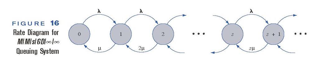
39 The no-memory property of the exponential distribution -> Probability that a customer will complete service between t and t + t is given by For j>=1, µj = µ If we assume that service completions and arrivals occur independently, then an M/M/1/FCFS/ / queuing system is a birth death process.

40 Consider an M/M/3/FCFS/ / queuing system in which interarrival times are exponential with λ= 4 and service times are exponential with µ = 5 A birth-death process

41 If either interarrival times or service times are nonexponential, then the birth death process model is not appropriate. A modified birth death model can be developed if service times and interarrival times are Erlang distributions.

42 Derivation of steady state probabilities for birth-death process Note that there are four ways for the state at time t + t to be j.

43 the probability that the state of the system will be j - 1 at time t and j at time t + t

44 Thus: Regrouping = o( t)

45 Dividing both sides by t and letting t approaches zero

46 Steady state: lim π = ( t ) ' ( t) = 0 t P ij P ij Thus, for j>=1 And for j=0

47 At any time t that we observe a birth death process, it must be true that for each state j, the number of times we have entered state j differs by at most 1 from the number of times we have left state j. Thus, for large t: Unit time Unit time

48 For j>=1 Unit time Unit time

49 Thus for j>=1 Thus for j>=1 Flow balance equations Conservation of flow equation

50

51 Solution of birth-death flow balance equations Begin by expressing all πj s in terms of π0

52 Define: Then: And

53 Hence: If j= j= 1 c j finite If not finite no steady state (arrival rate is at least as large as the maximum rate at which customers can be served.

54 Example 2: Indiana Bell Indiana Bell customer service representatives receive an average of 1,700 calls per hour.the time between calls follows an exponential distribution. A customer service representative can handle an average of 30 calls per hour. The time required to handle a call is also exponentially distributed. Indiana Bell can put up to 25 people on hold. If 25 people are on hold, a call is lost to the system. Indiana Bell has 75 service representatives. 1. What fraction of the time are all operators busy? 2. What fraction of all calls are lost to the system?

55 1. π 75 + π π 100 = π 100 =

56 M/M/1/GD/ / queuing system and queuing optimization model

57 The M/M/1/GD/ / Queuing System An M/M/1/GD/ / queuing system can be modeled as death birth process with parameters: Use equation (15) (19)

58 Define: ρ=λ/µ Substituting (21) into (17) Define S = (1+ρ+ ρ 2 + ρ 3...) ρs = ρ+ ρ 2 + ρ 3... S- ρs = 1

59 Thus If ρ>=1 then the system will blow up.

60 Derivation of L The average number of customers present in the queuing system (L) is given by: Defining:

61 Now

62 Derivation of Lq The expected number of people waiting in line (Lq) If j people are present the system, there will be j-1 people present in the line. Since L = ρ/(1- ρ)

63 Derivation of Ls The expected number of customers in server (Ls) We could have determined Lq from:

64 The queuing formula L = λw Little s queuing formula, define:

65 All averages are in the steady state:

66 For the M/M/1/GD/ / queuing system

67 Example 3: Drive in banking An average of 10 cars per hour arrive at a single-server drive-in teller. Assume that the average service time for each customer is 4 minutes, and both interarrival times and service times are exponential. Answer the following questions: 1. What is the probability that the teller is idle? 2. What is the average number of cars waiting in line for the teller? (A car that is being served is not considered to be waiting in line.) 3. What is the average amount of time a drive-in customer spends in the bank parking lot (including time in service)? 4. On the average, how many customers per hour will be served by the teller?

68 1. π0 = 1 - ρ = 1 2/3 = 1/3 2. We seek Lq: 3. We seek L: 1-2/3 Thus W = 2/10 =1/5 hour = 12 minutes. 4. If the teller were always busy then µ = 15. The teller is only busy 2/3rd of the time, thus he will serve an average of 2/3(15) = 10 customers.

69 Example 4: Service station Suppose that all car owners fill up when their tanks are exactly half full. At the present time, an average of 7.5 customers per hour arrive at a single-pump gas station. It takes an average of 4 minutes to service a car. Assume that interarrival times and service times are both exponential. Compute L and W! We have an M/M/1/GD/ / system λ = 7.5 cars per hr and µ = 15 cars/hr ρ = 0.50 L = 0.5/(1-0.5) = 1 and W = L/ λ = 1/7.5 = 0.13 hr.

70 Suppose that a gas shortage occurs and panic buying takes place. To model this phenomenon, suppose that all car owners now purchase gas when their tanks are exactly threequarters full. Since each car owner is now putting less gas into the tank during each visit to the station, we assume that the average service time has been reduced to 3 1/3 minutes. How has panic buying affected L andw? Now λ = 2(7.5) = 15 cars/hr (Each owner will fill up twice as often). µ = 60/3.333 = 18 cars/hr ρ = 5/6 1-5/6

71 As ρ approaches 1, L and W increase rapidly

72 A queuing optimization model

73 Example 5: Tool Center Machinists who work at a tool-and-die plant must check out tools from a tool center. An average of ten machinists per hour arrive seeking tools. At present, the tool center is staffed by a clerk who is paid $6 per hour and who takes an average of 5 minutes to handle each request for tools. Since each machinist produces $10 worth of goods per hour, each hour that a machinist spends at the tool center costs the company $10. The company is deciding whether or not it is worthwhile to hire (at $4 per hour) a helper for the clerk. If the helper is hired, the clerk will take an average of only 4 minutes to process requestsfor tools. Assume that service and interarrival times are exponential. Should the helper be hired?

74 The firms wants to hour hour customer hour Customer Machine-hr Customer hr

75 If the helper is not hired: λ = 10 machinists per hr, and µ = 12 machinist per hr W = 1/(12-10) = ½ hr. hour Expected cost per hr = = $56 With the helper: µ = 15 W = 1/(15-10) = 1/5 hour Expected cost per hr = (6+4) + 20 = $30 Should hire the helper

76 The queuing formula L = λw is very general and can be applied to many situations that do not seem to be queuing problems. Think of any situation where a quantity (such as mortgage loan applications, potatoes at McDonald s, revenues from computer sales) flows through a system. Note: Examples 6 and 7 are not discussed

77 Problems: Group A 4. A fast-food restaurant has one drive-through window.an average of 40 customers per hour arrive at the window. It takes an average of 1 minute to serve a customer. Assume that interarrival and service times are exponential. a) On the average, how many customers are waiting in line? b) On the average, how long does a customer spend at the restaurant (from time of arrival to time service is completed)? c) What fraction of the time are more than 3 cars waiting for service (this includes the car (if any) at the window)?

78 M/M/1/GD/c/ queuing system

79 Total capacity = c Parameters

80 Define ρ = λ/µ, using Eq the steady state is then given by When λ µ

81 If λ = µ, all c j s = 1, and all π j s equal

82 Thus: The actual arrival Even when λ µ, the system will never blow up.

83 Example 8: Barber shop A one-man barber shop has a total of 10 seats. Interarrival times are exponentially distributed, and an average of 20 prospective customers arrive each hour at the shop. Those customers who find the shop full do not enter. The barber takes an average of 12 minutes to cut each customer s hair. Haircut times are exponentially distributed. 1. On the average, how many haircuts per hour will the barber complete? 2. On the average, how much time will be spent in the shop by a customer who enters?

84 1. π 10 will leave the shop. An average of λ(1- π 10 ) will actually enters the shop. c = 10, λ = 20, µ = 5 ρ = 20/5 = 4 Thus an average of 20 (1-0.75) = 5 customers per hour will receive haircuts. or (20-5 =15) customers per hour will leave the shop.

85 2. To determine W, 20 (1-0.75)

86 A service facility consists of one server who can serve an average of 2 customers per hour (service times are exponential). An average of 3 customers per hour arrive at the facility (interarrival times are assumed exponential).the system capacity is 3 customers. a. On the average, how many potential customers enter the system each hour? b. What is the probability that the server will be busy?

87 The M/M/s/GD/ / queuing system

88 Assume that interarrival times are exponential (with rate λ), service times are exponential (with rate µ), and there is a single line of customers waiting to be served at one of s parallel servers. If j servers are occupied then service rate:

89 With parameters:

90 Define: ρ=λ/sµ yields the steady state probabilities: If λ 1 then no steady state exists.

91 The steady state probability that all servers are busy: It can be shown that: in queue

92 in the system

93

94 Example 9: Bank Tellers Consider a bank with two tellers. An average of 80 customers per hour arrive at the bank and wait in a single line for an idle teller. The average time it takes to serve a customer is 1.2 minutes. Assume that interarrival times and service times are exponential. Determine 1. The expected number of customers present in the bank 2. The expected length of time a customer spends in the bank 3. The fraction of time that a particular teller is idle

95 1. The system: M/M/2/GD/ / λ = 80, µ = 50, ρ = 80/2(5) = 0.8 <1 steady state exists From Table 6. P(j 2) = Since

96 3. Note that a particular server is idle during the entire time that j=0 and half the time (by symmetry) that j=1. Probability that a server is idle = π π 1 Probability that a server is idle = (0.176) = Note: We can use equation (39) to calculate π 0

97 Example 10: Bank Staffing The manager of a bank must determine how many tellers should work on Fridays. For every minute a customer stands in line, the manager believes that a delay cost of 5 is incurred. An average of 2 customers per minute arrive at the bank. On the average, it takes a teller 2 minutes to complete a customer s transaction. It cost the bank $9 per hour to hire a teller. Interarrival times and service times are exponential. To minimize the sum of service costs and delay costs, how many tellers should the bank have working on Fridays?

98 λ = 2 customer per minute, µ = 0.5 customer per minute Since ρ<1 : 2/s(0.5) <1 then s 5 Compute: Minute Minute Teller is paid : 9/60 = 15 cents per minute Expected service cost/minute = 0.15s. ($)

99 minute minute customer Where: customer Since average customers arrive per minute: minute

100 Now, for s=5 ρ = 2/5(0.5) = 0.80, P(j 5) = 0.55 minute minute For s = 6 Expected service cost per minute = 0.15(6) = 96 cents cannot have a lower cost than 5 tellers.

101 We need to know the distribution of a customer s waiting time The probability that a customer has to wait for more than 10 minutes: P(Wq> 10) = e -5(0.5)(1-0.8).10 = 0.004

102 The M/G/ /GD/ / and GI/G/ /GD/ / Models

103 An infinite server (self service) system in which a customer never has to wait for service to begin. 1. Interarrival times are iid with common distribution A. Define E(A) = 1/λ. Thus, λ = the arrival rate. 2. When a customer arrives, he or she immediately enters service. Each customer s time in the system is governed by a distribution S having E(S) = 1/µ.

104 Let L = the expected number of customers in the system (steady state) W = the expected time a customer spends in the system W = 1/ µ does not require any assumptions exponential distribution If interarrival times are exponential π j follows Poisson distribution

105 Example 11: Smalltown ice cream shops During each year, an average of 3 ice cream shops open up in Smalltown. The average time that an ice cream shop stays in business is 10 years. On January 1, 2525, what is the average number of ice cream shops that you would find in Smalltown? If the time between the opening of ice cream shops is exponential, what is the probability that on January 1, 2525, there will be 25 ice cream shops in Smalltown?

106 We are given: λ=3 shops per year, 1/µ = 10 years per shop. Assume that steady state exists: L = λ(1/µ) = 3 (10) = 30 shops in Smalltown If interarrivals are exponential:

107 M/G/1/GD/ / Queuing System

108 The system is not a birth-death process because service times no longer have the no-memory property. The Markov Chain theory is then used to determine: π i = the probability that after the system has operated for a long time, i customers will be present at the instant immediately after a service completion occurs. π i i = the fraction of the time after the system has operated for a long time that i customers are present. π ' i = π i

109 From Pollaczek and Khinchin: π ρ =1 0

110 Comparison: λ= 5, µ = 8 M/M/1/GD/ / M/D/1/GD/ / E(S) = 1/8 hr, Var (S) = 1/64 hr 2 E(S) = 1/8 hr, Var (S) = 0 a decrease in the variability of service times can substantially reduce queue size and customer waiting time

111 Finite Source Models: M/M/R/GD/K/K The Machine Repair Model

112 The system consists of K machines and R repair people. At any instant in time, a particular machine is in either good or bad condition. The length of time that a machine remains in good condition follows an exponential distribution with rate λ. Whenever a machine breaks down, the machine is sent to a repair center consisting of R repair people. The repair center services the broken machines as if they were arriving at an M/M/R/GD/ / system.

113 The time it takes to complete repairs on a broken machine is assumed exponential with rate µ. Once a machine is repaired, it returns to good condition and is again susceptible to breakdown.

114 A birth corresponds to a machine breaking down A death correponds to a machine having just been repaired. The total rate at which breakdowns occur when the state is j is:

115 Define ρ = λ/µ, the steady state probability is given by:

116 Determine the following:

117 The average number of arrival per unit time: We then obtain:

118 Example 12: Patrol cars The Gotham Township Police Department has 5 patrol cars. A patrol car breaks down and requires service once every 30 days. The police department has two repair workers, each of whom takes an average of 3 days to repair a car. Breakdown times and repair times are exponential. 1. Determine the average number of police cars in good condition. 2. Find the average down time for a police car that needs repairs. 3. Find the fraction of the time a particular repair worker is idle.

119 The machine repair problem: K =5, R = 2, λ = 1/30 car per day, and µ =1/3 car per day

120 1. The expected number of cars in good condition is K - L, which is given by 2. We seek L W = λ L W = = λ = days

121 3. The fraction of the time that a particular repair worker will be idle is π π 1 = (.310) = If there were R people, the probability that a particular server would be idle =

122 Exponential Queues in Series and Open Queuing Networks

123 Queues in series In many situations (such as the production of an item on an assembly line), the customer s service is not complete until the customer has been served by more than one server. a k-stage series (or tandem) queuing system

124 Assume that each stage must have sufficient capacity to service a stream of arrivals that arrives at rate λ; otherwise, the queue will blow up at the stage with insufficient capacity. Jackson s theorem λ < s µ j j

125 Example 13: Auto assembly The last two things that are done to a car before its manufacture is complete are installing the engine and putting on the tires. An average of 54 cars per hour arrive requiring these two tasks. One worker is available to install the engine and can service an average of 60 cars per hour. After the engine is installed, the car goes to the tire station and waits for its tires to be attached. Three workers serve at the tire station. Each works on one car at a time and can put tires on a car in an average of 3 minutes. Both interarrival times and service times are exponential. 1. Determine the mean queue length at each work station. 2. Determine the total expected time that a car spends waiting for service.

126 This is a series queuing system

127 Since λ < µ 1 and λ <µ 2 no system will blow up. ρ (for engine) = 54/60 = 0.9 ρ (for tire ) = 54/3 (20) = 0.9 The total expected time a car spends = = 0.288

128 Open queuing network Is a generalization of queues in series. Customers are assumed to arrive at station j from outside the queuing system at rate r j

129 Once completing service at station i, a customer joins the queue at station j with probability p ij and completes service with probability Define λ j, the rate at which customers arrive at station j (this includes arrivals at station j from outside the system and from other stations solved by:

130 Suppose s i µ j > λ j holds for all stations treating j as an M/M/sj /GD/ / system with arrival rate λ j and service rate µ j. If for some j, s j µ j λ j, then no steady-state distribution of customers exists. Remarkably, the numbers of customers present at each station are independent random variables. This result does not hold, however, if either interarrival or service times are not exponential.

131 To find L, the expected number of customers in the queuing system, simply add up the expected number of customers present at each station. To find W, the average time a customer spends in the system, simply apply the formula L = λw to the entire system. Here, λ = r 1 + r r k, because this represents the average number of customers per unit time arriving at the system.

132 Example 14: Open queuing networks Consider two servers. An average of 8 customers per hour arrive from outside at server 1, and an average of 17 customers per hour arrive from outside at server 2. Interarrival times are exponential. Server 1 can serve at an exponential rate of 20 customers per hour, and server 2 can serve at an exponential rate of 30 customers per hour. After completing service at server 1, half of the customers leave the system, and half go to server 2. After completing service at server 2, 3/4 of the customers complete service, and 1/4 return to server What fraction of the time is server 1 idle? 2. Find the expected number of customers at each server. 3. Find the average time a customer spends in the system. 4. How would the answers to parts (1) (3) change if server 2 could serve only an average of 20 customers per hour?

133 It is an open queuing network with r 1 =8 customers/hour and r 2 = 17 customers/hour. p 12 = 0. 5, p 21 = 0.25, and p 11 = p 22 = 0 λ = λ 1 λ = λ λ = 14 1 λ = Server 1 may be treated as an M/M/1/GD/ / system with λ = 14 customers/hour and µ =20 customers/hour. Then π 0 = 1 - ρ = = 0.3. Thus, server 1 is idle 30% of the time.

134 2. We find L at server 1 = = 7 3 L at server 2 = = 4 The average number of customers = 4 + 7/3 = 19/3

135 3. W = L/λ, where λ = = 25 customers per hour W = 19 / 3 25 = hour 4. No steady state because s 2 µ 2 = 20 < λ 2,

136 The M/G/s/GD/s/ System (Blocked Customers Cleared)

137 If arrivals who find all servers occupied leave the system, we call the system a blocked customers cleared, or BCC, system. Assuming that interarrival times are exponential, such a system may be modeled as an M/G/s/GD/s/ system Since a queue can never occur, Lq =Wq = 0 L,W, Lq andwq are of limited interest. Define 1 be the mean service time µ λ be arrival rate Then W = W s = 1 µ

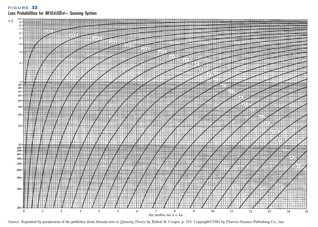
138 Primary interest is focused on the fraction of all arrivals who are turned away A fraction πs of all arrivals will be turned away An average of λ πs will be lost to the system. For an M/G/s/GD/s/ system, it can be shown that πs depends on the service time distribution only through its mean (1/µ). This fact is known as Erlang s loss formula.

139 In other words, any M/G/s/GD/s/ system with an arrival rate λ and mean service time of 1/µ will have the same value of πs. If we define ρ = λ /µ, then for a given value of s, the value of πs can be found from Figure 32.

140

141 Example 15: Ambulance calls An average of 20 ambulance calls per hour are received by Gotham City Hospital. An ambulance requires an average of 20 minutes to pick up a patient and take the patient to the hospital. The ambulance is then available to pick up another patient. How many ambulances should the hospital have to ensure that there is at most a 1% probability of not being able to respond immediately to an ambulance call? Assume that interarrival times are exponentially distributed.

142 See that λ = 20 calls per hour, and 1/µ = 1/3 hr. ρ = 20/3 = We seek the smallest value of s for which πs = 0.01 or smaller. s= 13 πs = 0.11 s = 14 πs = Thus, the hospital needs 14 ambulances.

143