DEPARTMENT OF QUANTITATIVE METHODS & INFORMATION SYSTEMS

Transcription

1 DEPARTMENT OF QUANTITATIVE METHODS & INFORMATION SYSTEMS Time Series and Their Components QMIS 320 Chapter 5 Fall 2010 Dr. Mohammad Zainal

2 2 Time series are often recorded at fixed time intervals. For example, Y might represent sales, and the associated time series could be a sequence of annual sales figures. Other examples of time series include quarterly earnings, monthly inventory levels, and weekly exchange rates. In general, time series do not behave like a random sample and require special methods for their analysis. Observations of a time series are typically related to one another (autocorrelated). This dependence produces patterns of variability that can be used to forecast future values and assist in the management of business operations. Consider these situations. It is important that managers understand the past and use historical data and sound judgment to make intelligent plans to meet the demands of the future.

3 3 Properly constructed time series forecasts help eliminate some of the uncertainty associated with the future and can assist management in determining alternative strategies. Forecasting is done by a set of procedures followed by judgments.

4 4 Decomposition It is an approach to the analysis of time series data involves an attempt to identify the component factors that influence each of the values in a series. The components of time series are: Time Series Trend Component Seasonal Component Cyclical Component Random Component

5 5 1. Trend Component It represents the growth and the decline in a time series, denoted by T. Long run increase or decrease over time (overall upward or downward movement) and they could linear or nonlinear Data taken over a long period of time

6 6 2. Cyclical Component It represents a long term wavelike fluctuations or cycles of more than one yearʹs duration in a time series, denoted by C. Practically it is difficult to identify and frequently regarded as part of trend. Regularly occur but may vary in length Often measured peak to peak

7 7 3. Seasonal Component It represents the seasonal variation in a time series which refers to a more or less stable pattern of change that appears short term regular wave like patterns and repeats itself season after season, denoted by S. Observed within 1 year. Often monthly or quarterly.

8 8 4. Irregular Component It represents the unpredictable or random fluctuations in a time series, denoted by I. Unpredictable, random, residual fluctuations Due to random variations of Nature Accidents or unusual events Noise in the time series To study the components of a time series, the analyst must consider how the components relate to the original series.

9 9 Time Series Components Models Additive Components Model It is suggested to use when the variability are the same throughout the length of the series. Multiplicative Components Model It is suggested to use when the variability are increasing throughout the length of the series. Note that it is possible to convert the multiplicative model to the additive model using logarithms. i.e.

10 10 Time series with constant variability

11 11 Time series with increasing variability

12 12 Estimation of Time Series Components Estimation of Trend Component Trends are long term movements in a time series that can be sometimes be described by a straight line or a smooth curve. Remark Fitting a trend curve helps us in providing some indication of the general direction of the observed series, and in getting a clear picture of the seasonality after removing the trend from the original series. The Linear Trend The Quadratic Trend

13 13 The Exponential Trend Where Tˆt is the predicted value of the trend at time t, b 0, b 1 and are called the model parameters. We can forecast the trend using the above models as and so on. Note that the Error Sum of Squares (SSE) is measured by

14 14 Example 5.1 Data on annual registrations of new passenger cars in the United States from 1960 to 1992 are shown in the following table and plotted in the later figure.

15 15 We definitely have a trend here!

16 16 The values from 1960 to 1992 are used to develop the trend equation. Registrations is the dependent variable, and the independent variable is time t coded as 1960 = 1, 1961 = 2, and so on. The fitted trend line has the equation The slope of the trend equation indicates that registrations are estimated to increase an average of 68,700 each year. The figure shows a straight line trend fitted to the actual data. It also shows forecasts of new car registrations for the years 1993 and 1994 (t = 34 and t = 35) obtained by extrapolating the trend line.

17 17 The estimated trend values for passenger car registrations from 1960 to 1992 are shown in the table. For example, the trend equation estimates registrations in 1992 (t =33) to be or 10,255,000 registrations. Registrations of new passenger cars were actually 8,054,000 in For 1992, the trend equation overestimates registrations by approximately 2.2 million. This error and the remaining estimation errors were listed in the table. The estimation errors were used to compute the measures of fit, MAD, MSD, and MAPE also were shown in the figure.

18 18 Forecasting a Trend Which trend model is appropriate? Linear, quadratic or exponential Linear models assume that a variable is increasing (or decreasing) by a constant amount each time period. A quadratic curve is needed to model the trend. Based on the accuracy measures, a quadratic trend appears to be a better representation of the general direction of the data.

19 19 When a time series starts slowly and then appears to be increasing at an increasing rate such that the percentage difference from observation to observation is constant, an exponential trend can he fitted. The coefficient b 1 is related to the growth rate. If the exponential trend is fit to annual data, the annual growth rate is estimated to be 100(b 1 1)%. The figure next contains the number of mutual fund salespeople for several consecutive years. The increase in the number of salespeople is not constant. It appears as if increasingly larger numbers of people are being added in the later years.

20 20 A linear trend fit to the salespeople data would indicate a constant average crease of about nine salespeople per year. This trend overestimates the actual increase in the earlier years and underestimates the increase in the last year. It does not model the apparent trend in the data as well as the exponential curve. It is clear that extrapolating an exponential trend with a 31 % growth rate will quickly result in some very big numbers. This is a potential problem with an exponential trend model. What happens when the economy cools off and stock prices begin to retreat? The demand for mutual fund salespeople will decrease and the number of salespeople could even decline. The trend forecast by the exponential curve will be much too high.

21 21 Growth curves of the Gompertz and logistic types reflect a situation in which sales begin low, then increase as the product catches on, and finally ease off as saturation is reached. Judgment and common sense are very important in selecting the right approach. As we will discuss later, the line or curve that best fits a set of data points might not make sense when projected as the trend of the future.

22 22 Suppose we are presently at time t = n (end of series) and we want to use a trend model to forecast the value of Y, p steps ahead. The time period at which we make the forecast, n in this case, is called the forecast origin. The value p is called the lead time. For the linear trend model, we can produce a forecast by evaluating Using the trend line fitted to the car registration data in Example 5.1, a forecast of the trend for 1993 (t = 34) made in 1992 (t = n = 33) would be the p = 1 step ahead forecast Similarly, the p = 2 step ahead forecast (1994) is given by

23 23 Using the quadratic trend curve for the car registration data, we can calculate forecasts of the trend for 1993 and 1994 by setting t = = 34 and t = = 35. The forecasts are = and = (respectively) Recalling that car registrations are measured in millions, the two forecasts of trend produced from the quadratic curve are quite different from the forecasts produced by the linear trend equation. Moreover, they are headed in the opposite direction. If we were to extrapolate the linear and quadratic trends for additional time periods, their differences would be magnified. This example illustrates why great care must be exercised in using fitted trend curves for the purpose of forecasting future trends. The differences can be substantial for large lead times (long run forecasting).

24 24 Trend curve models are based on the following assumptions: The correct trend curve has been selected. The curve that fits the past is indicative of the future. We must be able to argue that the correct trend has been selected the future will be like the past. There are objective criteria for selecting a trend curve. We will discuss two of these criteria, the Akaike Information Criterion (AIC) and the Bayesian Information Criterion (BIC), in later chapters. However, although these and other criteria help to determine an appropriate model, they do not replace good judgment.

25 25 Estimation of Seasonal Component A seasonal pattern is one that repeats itself year after year. For annual data, seasonality is not an issue because there is no chance to model a within year pattern with data recorded once per year. Time series consisting of weekly, monthly, or quarterly observations often exhibit seasonality. The analysis of the seasonal component of a time series has direct shortterm implications and is of greatest importance to mid and lower level management. Marketing plans have to take into consideration expected seasonal patterns in consumer purchases. Several methods for measuring seasonal variation have been developed. The basic idea in all of these methods is to first estimate and remove the trend from the original series and then smooth out the irregular component.

26 26 The seasonal values are collected and summarized to produce a number (generally an index number) for each observed interval of the year (week, month, quarter, and so on). The identification of the seasonal component in a time series differs from trend analysis in at least two ways: 1. The trend is determined directly from the original data, but the seasonal component is determined indirectly after eliminating the other components from the data so that only the seasonality remains. 2. The trend is represented by one best fitting curve, or equation, but a separate seasonal value has to be computed for each observed interval (week, month, quarter) of the year and is often in the form of an index number. Always we estimate the seasonality in form of index numbers, percentages that show changes over time, are called seasonal index. If an additive decomposition is used, estimates of the trend, seasonal, and irregular components are added together to produce the original series.

27 27 If a multiplicative decomposition is used, the individual components must be multiplied together to reconstruct the original series, and in this formulation, the seasonal component is represented by a collection of index numbers. These numbers show which periods within the year are relatively low and which periods are relatively high. The seasonal indices trace out the seasonal pattern. Index numbers are percentages that show changes over time. Remark In this chapter we study the multiplicative model and leave the additive model to chapter 8 if we have time. In multiplicative decomposition model, the ratio to moving average is a popular method for measuring seasonal variation.

28 28 Finding Seasonal Indexes Ratio to moving average method: Begin by removing the seasonal and irregular components (S t and I t ), leaving the trend and cyclical components (T t and C t ) Example: Four quarter moving average First average: Second average: Moving average 1 = Q1+ Q2 + Q3 + Q4 4 etc Moving average 2 Q2 + Q3 + Q4 + Q5 = 4

29 29 Quarter 1 Sales 23 Quarterly Sales Sales Quarter etc etc

30 30 Centered Seasonal Index Quarter Sales etc Average Period 4-Quarter Moving Average = = 4 Each moving average is for a consecutive block of 4 quarters

31 31 Average periods of 2.5 or 3.5 don t match the original quarters, so we average two consecutive moving averages to get centered moving averages Average Period 4-Quarter Moving Average etc Centered Period Now estimate the S t x I t value by dividing the actual sales value by the centered moving average for that quarter. QMIS 320, CH 5 by M. Zainal Centered Moving Average

32 32 Ratio to Moving Average formula: S t It = T t Yt C t Quarter Sales Centered Moving Average Ratio-to- Moving Average etc etc Example = 29.88

33 33 Quarter Sales Centered Moving Average Ratio-to- Moving Average Fall Average all of the Fall values to get Fall s seasonal index Fall Do the same for the other three seasons to get the other seasonal indexes Fall etc etc

34 34 Suppose we get these seasonal indices: Season Seasonal Index Interpretation: Spring Summer Fall Spring sales average 82.5% of the annual average sales Summer sales are 31.0% higher than the annual average sales etc Winter Σ = four seasons, so must sum to 4 QMIS 320, CH 5 by M. Zainal

35 35 The data is deseasonalized by dividing the observed value by its seasonal index Yt Tt Ct It = S This smoothes the data by removing seasonal variation t Quarter Sales Seasonal Index Deseasonalized Sales =

36 36

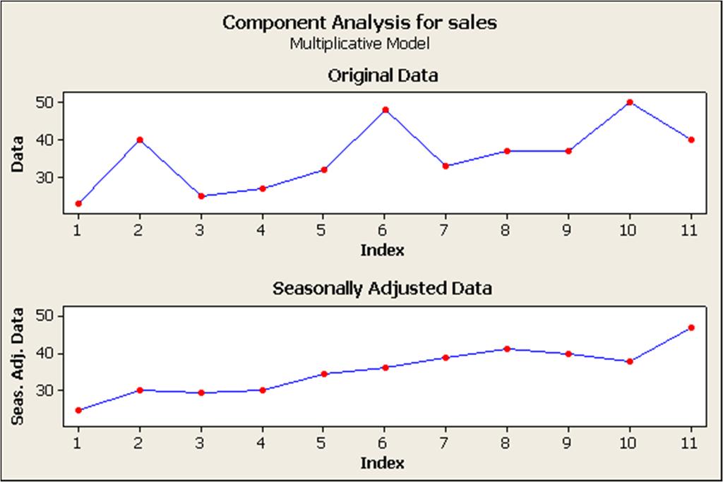
37 37 Example 5.3 In Example 3.5 the analyst for the Outboard Marine Corporation, used autocorrelation analysis to determine that sales were seasonal on a quarterly basis. Now, he uses decomposition to understand the quarterly sales variable. Minitab was used to produce the following table and figure. To keep the seasonal pattern current, only the last seven years (1990 to 1996) of sales data (Y), were analyzed. The trend is computed using the linear model:

38 38 I= CI/ C = /1.146 = T = + = SCI = Y T = =.912 S = ( ) 7 = ˆ (1) TCI = Y S = = CI = Y TS = ( ) C = ( ) 3 = 1.146

39 39 The cyclical indices can be used to answer the following questions: The series cycle? How extreme is the cycle? The series follow the general state of the economy (business cycle)? One way to investigate cyclical patterns is through the study of business indicators. A business indicator is a business related time series that is used to help assess the general state of the economy. The most important list of statistical indicators originated during the sharp business setback of 1937 to Leading indicators. Coincident indicators. Lagging indicators.

40 40 Forecasting A Seasonal Time Series In forecasting a seasonal time series, the decomposition process is reversed. Instead of separating the series into individual components for examination, the components are recombined to develop the forecasts for future periods. Example 5.4 Forecasts of Outboard Marine Corporation sales for the four quarters of 1997 can he developed using the previous table. 1. Trend. The quarterly trend equation is: T = t. The forecast origin is the fourth quarter of 1996, or time period t = n = 28. Sales for the first quarter of 1997 occurred in time period t = = 29. This notation shows we are forecasting p = 1 period ahead from the end of the time series. Setting t = 29, the trend projection is then T 29 = (29) =

41 41 2. Seasonal. The seasonal index for the first quarter is Cyclical. The cyclical projection must be determined from the estimated cyclical pattern (if any) and any other information generated by indicators of the general economy for Projecting the cyclical pattern for future time periods is fraught with uncertainty, and as we indicated earlier, is generally assumed for forecasting purposes to be included in the trend. To demonstrate the completion of this example, we set the cyclical index to Irregular. Irregular fluctuations represent random variation that can t be explained by the other components. For forecasting, the irregular component is set to the average value 1.0 The forecast for the first quarter of 1997 is The forecasts for the rest of 1997 are