We need to talk about about Kevin

Transcription

1 Professor Kostas Nikolopoulos, D.Eng., ITP, P2P Chair in Business Analytics Prifysgol Bangor University We need to talk about about Kevin joint work with many friends

2

3 It does not exist An economist s view

4 Aggregation/Hierarchies Temporal Spatial Family

5 The spike.

6

7 Is it me Or are we keep on looking in the same thing?

8

9 A conceptual framework to synthesise those thoughts

10 Two important concepts The level of decision making (temporal spatial family). The level where I can achieve maximum forecastability (and still of course generate forecasts at the desired level)

11 Forecasting Black & White Swans joint work with Fotios Petropoulos (Bath)

12 Black (White & Gray) Swans White Swans the mainstream Indeed the normal is often irrelevant Gray Swans rare but expected (Taleb 2007) Somewhat predictable, particularly to those who are prepared for them and have the tools to understand them Black Swans the unexpected fewer remote events, but are more and more extreme in their impact

13 Black Swans according to Taleb the Problem is that people tend to theorize, explain things, or talk about random events with plenty of because in their conversation (about Black Swans)

14 (Learning? from) Historic Analogies

15 3.21% 3.21% 3.21% 3.21% 3.21% 3.21% 3.21% 3.21% 3.21% 3.21% 3.21% 3.21% 3.21% 3.21% 3.21% 3.21% 3.21% 3.21% 3.21% 3.21% 3.21% 3.21% 3.21% 3.21% 3.21% 3.21% 3.21% 3.21% 3.21% 3.21% 3.21% 3.21% 3.21% 3.21% 3.21% 3.21% 3.21% 3.21% 3.21% 3.21% 3.21% 3.21% 3.21% 3.21% 3.21% 3.21% 3.21% 3.21% 3.21% 3.21% 3.21% 3.21% 3.21% 3.21% 3.21% 3.21% 3.21% 3.21% 3.21% 3.21% 3.21% 3.21% 3.21% 3.21% 3.21% 3.21% -3.16% -3.16% -3.16% -3.16% -3.16% -3.16% -3.16% -3.16% -3.16% -3.16% -3.16% -3.16% -3.16% -3.16% -3.16% -3.16% -3.16% -3.16% -3.16% -3.16% -3.16% -3.16% -3.16% -3.16% -3.16% -3.16% -3.16% -3.16% -3.16% -3.16% -3.16% -3.16% -3.16% -3.16% -3.16% -3.16% -3.16% -3.16% -3.16% -3.16% -3.16% -3.16% -3.16% -3.16% -3.16% -3.16% -3.16% -3.16% -3.16% -3.16% -3.16% -3.16% -3.16% -3.16% -3.16% -3.16% -3.16% -3.16% -3.16% -3.16% -3.16% -3.16% -3.16% -3.16% -3.16% -3.16% Black (White & Gray) Swans 12% 10% 8% 6% 4% % Changes in Daily DJIA: Sept.15 to Dec. 1, 2008 (Parallel lines indicate the ± % CI, assuming normality) % of Days Outside the % Confidence Intervals: 52.7% 3.86% 3.35% 4.68% 11.08% 4.68% 4.67% 10.88% 3.28% 6.67% 6.54% 4.93% 3.31% 3.46% 4.20% 2% 0% -2% 09/15/08 09/17/08 9//08 09/23/08 09/25/08 09/29/08 10/01/08 10/03/08 10/07/08 10/09/08 10/13/08 10/15/08 10/17/08 10/21/08 10/23/08 10/27/08 10/29/08 10/31/08 11/04/08 11/06/08 11/10/08 11/12/08 11/14/08 11/18/08 11//08 11/24/08 11/27/08 12/01/08 12/03/08 12/05/08 12/09/08 12/11/08 12/15/08-4% -3.27% -3.22% -3.58% -4.42% -4.06% -5.11% -6% -5.69% -3.62% -4.85%-4.73% -5.05% -3.82% -5.07% -5.56% -8% -6.98% -7.33% -7.87% -7.70%

16 a decomposition lens S&P Index, Log Diffs of Weekly Closing Values 1/1/1990-1/2/2009

17 a decomposition lens

18 a decomposition lens

19 Scientists are dealing with this kind of data for more than??? years. Intermittent Demand

20 Accessed on 05 Aug 2010

21 How difficult this problem (really) is?

22 Croston s Approach (ORQ- 1971) Demand Forecast = (Volume Forecast) / (Interval Forecast) where: (Interval Forecast) = the exponentially smoothed (or moving average) inter-demand interval, updated only if demand occurs in period, and (Volume Forecast) = the exponentially smoothed (or moving average) size of demand, updated only if demand occurs in period

23 an interesting idea Non-overlapping Temporal Aggregation

24 Advantages and disadvantages The accumulation of demand observations in lower-frequency time buckets reduces the number of zero demands and the resulting series bear a greater resemblance to fast-moving items ouse methods originally designed for fast moving items An obvious disadvantage related to temporal aggregation is that of losing information since the frequency and number of observations is reduced. But in an intermittent series you did not got much information in the first place anyway, eh?

25 Optimum aggregation level for one time series? 5000 SKUs -RAF Data

26 Aggregation level = LT+R... a managerial-driven heuristic

27 Aggregation level = LT+R We have also examined the performance of ADIDA when the aggregation level matches the forecast horizon required for stock control purposes CumError = Cumulative Demand over LT Forecast over LT + 1 Forecasts ADIDA Forecasts 4,352 SKUs Bias Naïve SBA Naïve SBA ME MdE Accuracy MAsE % 92.13% 99.84% 89.24% MdAsE 13.04% 20.93% 19.56% 19.65% Uncertainty MSE

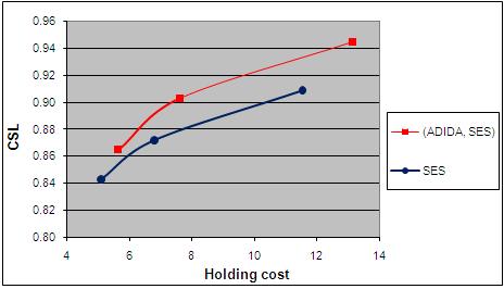
28 Economic significance (stock control) performance

29 3.21% 3.21% 3.21% 3.21% 3.21% 3.21% 3.21% 3.21% 3.21% 3.21% 3.21% 3.21% 3.21% 3.21% 3.21% 3.21% 3.21% 3.21% 3.21% 3.21% 3.21% 3.21% 3.21% 3.21% 3.21% 3.21% 3.21% 3.21% 3.21% 3.21% 3.21% 3.21% 3.21% 3.21% 3.21% 3.21% 3.21% 3.21% 3.21% 3.21% 3.21% 3.21% 3.21% 3.21% 3.21% 3.21% 3.21% 3.21% 3.21% 3.21% 3.21% 3.21% 3.21% 3.21% 3.21% 3.21% 3.21% 3.21% 3.21% 3.21% 3.21% 3.21% 3.21% 3.21% 3.21% 3.21% -3.16% -3.16% -3.16% -3.16% -3.16% -3.16% -3.16% -3.16% -3.16% -3.16% -3.16% -3.16% -3.16% -3.16% -3.16% -3.16% -3.16% -3.16% -3.16% -3.16% -3.16% -3.16% -3.16% -3.16% -3.16% -3.16% -3.16% -3.16% -3.16% -3.16% -3.16% -3.16% -3.16% -3.16% -3.16% -3.16% -3.16% -3.16% -3.16% -3.16% -3.16% -3.16% -3.16% -3.16% -3.16% -3.16% -3.16% -3.16% -3.16% -3.16% -3.16% -3.16% -3.16% -3.16% -3.16% -3.16% -3.16% -3.16% -3.16% -3.16% -3.16% -3.16% -3.16% -3.16% -3.16% -3.16% So how can this idea be used in a (Black & Gray) Swans context? 12% 10% 8% 6% 4% % Changes in Daily DJIA: Sept.15 to Dec. 1, 2008 (Parallel lines indicate the ± % CI, assuming normality) % of Days Outside the % Confidence Intervals: 52.7% 3.86% 3.35% 4.68% 11.08% 4.68% 4.67% 10.88% 3.28% 6.67% 6.54% 4.93% 3.31% 3.46% 4.20% 2% 0% -2% 09/15/08 09/17/08 9//08 09/23/08 09/25/08 09/29/08 10/01/08 10/03/08 10/07/08 10/09/08 10/13/08 10/15/08 10/17/08 10/21/08 10/23/08 10/27/08 10/29/08 10/31/08 11/04/08 11/06/08 11/10/08 11/12/08 11/14/08 11/18/08 11//08 11/24/08 11/27/08 12/01/08 12/03/08 12/05/08 12/09/08 12/11/08 12/15/08-4% -3.27% -3.22% -3.58% -4.42% -4.06% -5.11% -6% -5.69% -3.62% -4.85%-4.73% -5.05% -3.82% -5.07% -5.56% -8% -6.98% -7.33% -7.87% -7.70% The optimum temporal aggregation level may be the seen as the forecasting horizon within which we may be able to forecast appearance of a gray swan and thus plan how to respond to (even a Black one!)

30 What is the alternative? Extreme Value Theory (EVT) >>> is dealing with the extreme deviations from the median of probability distributions, in order to estimate the probability of events that are more extreme than anything in the past Two approaches mainly exist: deriving max/min series as a first step, i.e. generating an "Annual Maxima Series" (AMS) usually leading to the Generalized Extreme Value Distribution being fitted. Given that the number of relevant random events within a year usually is limited, very often analyses of observed AMS data lead to other distributions. Extracting values that exceed a certain threshold, usually referred to as "Point Over Threshold" (POT) method and can lead to several or no values being extracted in any given year. The analysis involves fitting two distributions: one for the number of events in a basic time period (usually Poisson) and a second for the size of the exceedances(usually a Generalized Pareto Distribution).

31 More aggregation Temporal Spatial Family

32 Case studies #1 Extreme Events and Risk Mitigation

33 Questions When you can NOT forecast what do you do in terms of planning? (MTO/MTS/?) To stock or not to Stock? That is the question

34

35

36

37

38 One critical variable

39 Another (critical) variable)

40

41

42 Case studies #2 More Regular Events and Pricing

43

44 How do you decide how to price Your insurance policies based in where your client frequently travels? Just what happened last year (naïve) or based on where you can forecast better? Temporal- spatial windows

45 Case studies #3 Very regular Events and Planning

46

47

48

49

50 Case studies #4 (really) Difficult Supply chains

51

52 Case studies #5 (really) Difficult Supply chains Part 2

53 Selling Sand to the Arabs aka MTO -> MTS transistions Kostas Nikolopoulos Chris Davies Siwan Michelmore A Forecasting Improvement project in a Food Processing SME (c100 staff)

54 Temporal Aggregations and Forecasting at FoodCo FoodCo are a local SME producing high quality frozen pre cooked meals. Their main customers are wholesale suppliers, who then supply pub chains, restaurants, and other vendors. FoodCo has a one site facility that cooks and stores all it s products. It is a highly regulated facility and there is full traceability throughout the production process. The company uses Information Technology to monitor and record customer orders, production status, and inventory levels.

55 Temporal Aggregations and Forecasting at FoodCo The company approached forlab to develop forecasting into it s production process with the aim to reduce inventory holdings, level production, and estimate future raw material requirements. Initially, the bulk of the production process was done under a Make to Order paradigm. With a small amount of products being produced as Make to Stock, in this case the level of inventory was set by the customer. As orders typically gave around twice the production lead time before the due date the MTO paradigm worked from the production perspective. However, it did make longer term raw material planning difficult, and the same with staff planning on longer horizons. Despite no formal forecasting being used the production and purchasing managers did employ informal heuristics, based on long term experience, to guesstimate what future demands could be.

56 Temporal Aggregations and Forecasting at FoodCo Rather than relying on informal heuristics, forlab proposed that FoodCo adopts a hybrid production methodology that combines both Make to Order and Make to Stock paradigms. And then use formal forecasting methods to assess how much product to make for the Make to Stock cohort. This required two key components, how to determine which product fits into which cohort and then what is the most appropriate forecasting method to use for the Make to Stock cohort product. In order to do this we first looked at the product order (demand) histories to asses how intermittent the demand is. The product demand histories came in a weekly format taken off the companies accounting database. This is important as intermittent data has a limited range of potential forecasting models, and makes selecting which products to place in which cohort difficult.

57 Temporal Aggregations and Forecasting at FoodCo On inspection it was found that the weekly data was intermittent by varying degrees. This left open two options Continue to work with the intermittent data, or to aggregate the data so that it becomes non intermittent. It was decided to aggregate the products demand so as to take advantage of the wider range of forecasting models and to enable a selection process. Nikolopoulos et al (2011) proposed the ADIDA (Aggregate Disaggregate Intermittent Demand Approach) framework that aggregates the data, thus allowing a wider range of forecasting models, and then disaggregates the forecast back to the original frequency.

58 Temporal Aggregations and Forecasting at FoodCo This produced a single layer hierarchy, by aggregating the weekly data into monthly data. In almost all cases this produced non intermittent time series. This enabled the selection process based on the products average demand and it s coefficient of variation. Forecasting was then employed on the Make to Stock cohort. disaggregated back to the weekly level. After the forecasting the results where

59 Product No Month 1 Month 2 Month 3 Average 1 8% 45% 0% 17.6% 2 17% 9% 14% 13.2% 3 15% 21% 21% 18.8% 4 22% 168% - 60% 5 30% 68% 1% 32% 6 52% 42% 17% 36% 7 8% 12% 14% 11.2% 8 59% 42% 2% 35% 9 40% 55% 42% 45% 10 12% 14% 11% 12.2% 11 22% 28% 1% 16% 12 16% 4% 3% 8% Absolute percentage error of monthly forecasts, and the MAPE, The average error being 25.47%

60 Temporal Aggregations and Forecasting at FoodCo As an example of the process, The weekly data was aggregated into monthly data to remove the intermittency. Monthly forecasts where generated, and then disaggregated back to the weekly level. This is how much gets produced each week to be kept in stock. Any surplus inventory is then kept for the following months orders. The production planner makes a judgement on how to adjust the following months forecast based on how much surplus inventory there is. If there is un forecasted demand, then the extra amount over the forecasted value is treated as Make to Order.

61 Temporal Aggregations and Forecasting at FoodCo For product 12 this ran thus.. Month 1 Forecasted monthly figure 1868 units disaggregated to 431 units each week. Actual monthly demand was 2242 so an extra 374 units was added to the production plan that month. Month 2 forecasted monthly figure 1871 units disaggregated to 432 units each week. Actual monthly demand was 1790 so this left a surplus of 81 units. This was kept over for the following month. Month 3 forecasted monthly figure 1861 units disaggregated to 429 units each week. Actual monthly demand was 1802 so this left a surplus of 59 units. It was decided that the combined surplus of 140 units would be rolled over to the following month as it was an established high demand month.

62 Temporal Aggregations and Forecasting at FoodCo For product 2 it ran thus.. Month 1 Forecasted monthly demand of 734, disaggregated to 170 units a week. Actual monthly demand was 880 units, so an extra 146 units was added to the production plan as MTO. Month 2 Forecasted monthly demand of 803, disaggregated to 185 units a week. Actual monthly demand was 880 units, so an extra 77 units was added to the production plan as MTO. Month 3 forecasted monthly demand was 849, disaggregated to 196 units a week. Actual monthly demand was 990 units, so an extra 141 units was added to the production plan as MTO. It was decided to add an extra 50 units a month to the forecast as the forecasts consistently undershot the actual demand.

63 Temporal Aggregations and Forecasting at FoodCo As can be seen between the two examples the forecasts can undershoot or exceed the actual demand. However, when the forecasts undershoot the actual demand this isn t so much of an issue as the forecasted amount has already produced a substantial portion of the actual demand. As most orders generally give a lead time that is twice the product lead time this means any un forecasted demand can be added to the pre planned weekly production level. The facility can produce runs in individual units or in thousands of units so the capacity is there to handle the unexpected extra demand. The forecasting means that there is less sudden demand on the production plan, which makes planning easier. Also, this planning has a positive effect for the purchasing department as they can see the following months plan and know how much to purchase to cover the forecasted demand.

64 Temporal Aggregations and Forecasting at FoodCo In conclusion, temporal aggregation has helped FoodCo to be more pre-emptive in their planning, rather than constantly reacting to demands. This enables a longer horizon on the production plans and can improve on response times to customer orders. It also enables better purchasing decisions for the raw materials required. Some raw materials have a long lead time on delivery so forward planning helps inform purchasing plans. Aggregation also enables a wider range of forecasting models to be used in predicting demand. The top down approach is also intuitively straightforward for the production planner use. As the process is done each month, any extra demand is only a small portion of the overall demand so there is little extra MTO demand on the plan. It also means the forecasts can react to changing demands in a more timely fashion.

65 So

66