Decision support models in the electric power industry

Transcription

1 ESCUELA TÉCNICA SUPERIOR DE INGENIERÍA ICAI EMIN: International Master in Economics and Management of Network Industries Decision support models in the electric power industry Bulk system reliability Andrés Ramos Session MOD.10

2 Bibliography IEEE Tutorial Course on Reliability Assessment of Composite Generation and Transmission Systems. IEEE October 1989 EPRI Composite-system reliability evaluation. EPRI EL December 1987 Rivier, M. (1998) Modelo probabilista de explotación de un sistema eléctrico: contribución a la teoría marginalista. Tesis doctoral. Universidad Pontificia Comillas. Sánchez, P. (1998) Mejoras en la eficacia computacional de modelos probabilistas de explotación generación/red a medio plazo. Tesis doctoral.. ( 2

3 Content Motivation and applications Probabilistic operation models Uncertainty modeling Some models 3

4 Motivation To give an indication about what it is possible to state with a decision tool Capabilities and limitations To become familiar with network modeling techniques To give the mathematical foundation 4

5 Long term applications Network expansion planning Selection and evaluation of network investments Impact on the generation equipment and consumption Interconnections 5

6 Medium term applications Traditional environment Studies about network performance Generation localization Adequacy assessment/reliability studies Network maintenance Operation planning TPA or open access Check transfer capabilities Determine payment for the network use Assign network costs Network remuneration studies Evaluate network contracts 6

7 Short term applications Check the viability of the generation and consumption dispatch Determine nodal marginal prices Identify and determine losses Identify and determine zonal or local ancillary services Decisions about network operation 7

8 Very short term applications Static analysis of the network Flows Voltages Dynamic analysis of the network Stability Voltage collapse 8

9 Model hierarchy _ + System detail Uncertainty + _ Very short term Short term Medium term Long term Time horizo on Operation scenario analysis Operation scenario probabilistic analysis Operation scenario probabilistic analysis Investment selection and analysis 9

10 Content Motivation and applications Probabilistic operation models Uncertainty modeling Some models 10

11 Methods Important developments in the field of reliability studies taking into account the transmission network Adequacy assessment Extension to cost studies 11

12 General structure Uncertainty Demand Hydrology Equipment unavailability Demand Hydro energy available Committed units System configuration Analysis of operation snapshots Results Cost evaluation Reliability indexes Economic indexes Technical indexes Sensitivities 12

13 Methods Generation + Network Single node generation Simulation Analytical methods (probabilistic simulation) Sampling Monte Carlo simulation (cost-reliability) Enumeration (reliability) Chronological - Sequential Random 13

14 Electric network subsystem Single node Generation/transmission Transportation model (1st Kirchoff s law) DC optimal power flow with or without losses AC optimal power flow Dynamic aspects Circuits Branches: lines and transformers. Nodes: substation buses. 15

15 Security criterion in contingency dispatch Preventive Network and/or generation margin, N-1. Representation in the dispatch model (global optimization, relaxation, scenarios, reserve markets and interruptibility) Corrective Generation response margins Load redistribution 16

16 Other characteristics to model Networks operating limits: Line thermal limits. Node voltages limits. Interruptible contracts Network emergency operation: e.g., tie and untie, substation reconfiguration Violation of preventive security regular criteria in special states (e.g., high cost, emergency) Reserves Exogenous criteria that condition the dispatch optimality (e.g., fuel quota) 18

17 Generation dispatch model Optimization Simulation + heuristics Sampling of random parameters Logic rules and pre-established strategies to optimize the decisions 19

18 Content Motivation and applications Probabilistic operation models Uncertainty modeling Some models 20

19 Uncertainty treatment Sources Demand Contingencies (availability of generation and network elements) Unregulated inflows or hydro outputs Enumeration is not possible by the huge number of states Monte Carlo simulation 21

20 How many samples are needed? Let s suppose that 25 samples are enough to determine the mean with a small enough confidence interval Failure probability for a generator: 5 % for a line: 0.5 % If I want to obtain 25 samples of a generator failure I ll need 500 samples a line failure I ll need 5000 samples Therefore, I ll need at least 5000 samples to obtain failures in lines and perhaps non served energy in certain nodes A strong computational effort is needed 22

21 Stages in Monte Carlo simulation 1. Pseudorandom number generation 2. Random variable generation 3. Simulation or parameter sampling 4. (Variance reduction techniques) 5. Results collection 6. Sampling process stop 23

22 Composite operation model SET cl Line characteristics /r, x, pmax, efor/ Line equivalent forced outage rate SET samples number of samples / 1 * 5000 / t_aux(g) thermal units h_aux(g) hydro units ii_aux(i,i) nodes connected by a line Number of samples SCALAR samplevalue sample value PARAMETERS efor(g) unit equivalent forced outage rate [p.u.] POSITIVE VARIABLES pns(i) power non served [GW] Unit equivalent forced outage rate Power non served E_FOBJ.. fobj =E= SUM[t, f(t) * alfa(t) * q(t) / k(t) + o(t) * q(t)] + SUM[h, c(h) * [q(h) - rend(h) * b(h)]] + 300*sum sum[i, pns(i)]; E_DMND(i).. SUM[t $ it(i,t), q(t)] + SUM[h $ ih(i,h), q(h) - b(h)] - SUM[j $ ii(i,j), p(i,j)] + SUM[j $ ii(j,i), p(j,i)] =E= d(i) - pns(i) ; pns.up(i) = d(i) ; PNS bound PNS cost in the objective funct PNS in demand equation 24

23 Monte Carlo simulation loop * Initialization of auxiliary sets ii_aux(i,j) = ii(i,j) ; t_aux(g) = t(g) ; h_aux(g) = h(g) ; * Loop for all the samples LOOP (samples, ii(i,j) = ii_aux(i,j) ; t(g) = t_aux(g) ; h(g) = h_aux(g) ; * Sample of thermal unit availability LOOP (t_aux(g), samplevalue = uniform(0,1) ; t(g) $[samplevalue < efor(g)] = no ; ) ; * Sample of hydro unit availability LOOP (h_aux(g), samplevalue = uniform(0,1) ; h(g) $[samplevalue < efor(g)] = no ; ) ; * Sample of line availability LOOP (ii_aux(i,j), samplevalue = uniform(0,1) ; ii(i,j) $[samplevalue < dtl(i,j,'efor')] = no ; ) ; * Solving the problem SOLVE MGR USING LP MINIMIZING fobj; Sample loop Thermal unit availability Hydro unit availability Line availability DC optimal power flow solution Escuela Técnica Superior de Ingeniería $ INCLUDE ICAI MSE_MGR_RESULTADOS.INC ) ; 25

24 Monte Carlo simulation (I) It is used when the number of states of the random parameters is very huge (e.g., contingencies) Estimate the mathematical expectation of operating costs and/or reliability measures Simulate is equivalent to integrate or sample in hyperspace of random parameters with a known probability density function Determine sample mean, mean variance, confidence interval. Stop sampling when confidence interval is lower than a certain tolerance. 26

25 Monte Carlo simulation (II) Quadratic behavior (4 times more samples divides by 2 the confidence interval) Events with a small probability and a huge value of the objective function cause high variances (it is the usual case of reliability indexes). Therefore, many samples are needed Variance reduction techniques Common random numbers, antithetic variables, control variable, importance sampling, stratified sampling Allow to reduce the size of the confidence interval of the mean without disturbing its value for a certain number of samples or, alternatively, achieve the desired precision with a lower sampling effort. 27

26 Variance reduction techniques VRT (I) Usually, it is impossible to know in advance the variance reduction to be achieved, or even if it is going to be reduced. We have to experiment considering the real system to analyze. You have to know the model in detail that reproduces the system behavior. The use of VRT can be understood as a way of taking advantage of information about the implied system. Imply a computational over-cost to do certain preliminary samples or auxiliary computations in the same simulation process. 28

27 Variance reduction techniques VRT (II) Common random numbers or correlated sampling or comparative simulation or synchronized pairs Do sampling for different system configurations with the same set of random numbers being used each one for the same function in sampling process. Antithetic variables It is based on the idea of introducing a negative correlation between two consecutive samples. It consists of the use of complementary random numbers in two consecutive simulations. 29

28 Variance reduction techniques VRT (III) Control variable The basic idea is to use the results of a simpler model to predict or explain part of the variance of the value to estimate. A previous computation of the expected value of the control variable is needed. This computation has to be very quick compared to those of the variable to estimate. Importance sampling The random variable to estimate is replaced by another with the same mean but different variance. The probability density function used in the sampling process is modified to center it around the area of interest. Sampling probable but not interesting events is avoided. 30

29 Variance reduction techniques VRT (IV) Stratified sampling The intuitive idea of this technique is similar to the previous one but in a discrete version. It consists on taking more samples of the random variable in the areas of greater interest. The variance is reduced by concentrating the simulation effort in the more relevant strata. 31

30 Content Motivation and applications Probabilistic operation models Uncertainty modeling Some models 32

31 Some IIT transmission network planning models Medium term application StarNet/RD for different companies in Dominican Republic SIMUSIS/SIMUMER/SIMUPLUS for REE Long term application PERLA/CHOPIN for REE 33

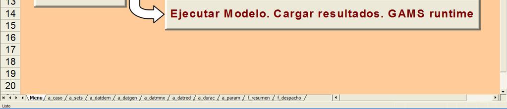
32 StarNet/RD (i) ( 34

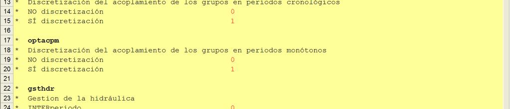
33 StarNet/RD (ii) 35

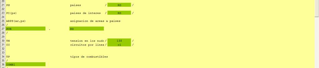
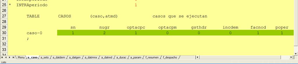
34 StarNet/RD (iii) 36

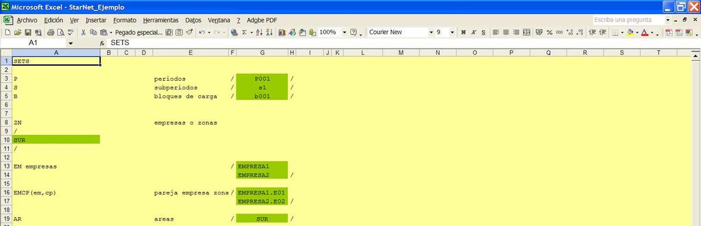
35 StarNet/RD (iv) 37

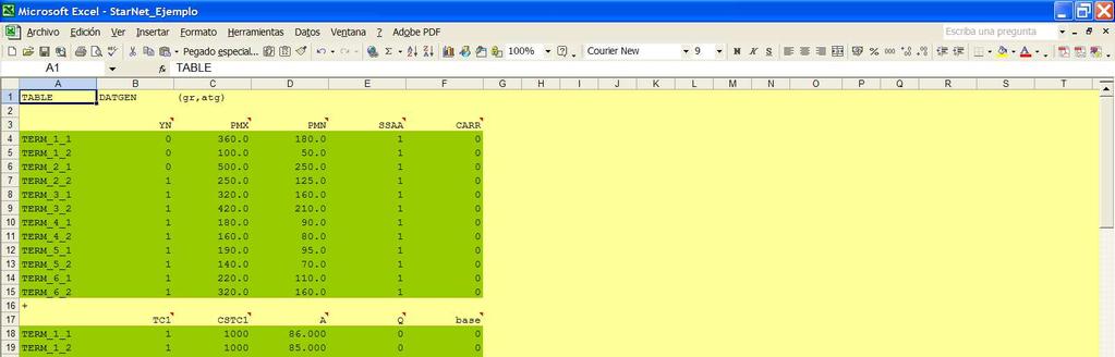
36 StarNet/RD (v) 38

37 StarNet/RD (vi) 39

38 StarNet/RD (vii) 40

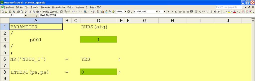
39 StarNet/RD (viii) 41

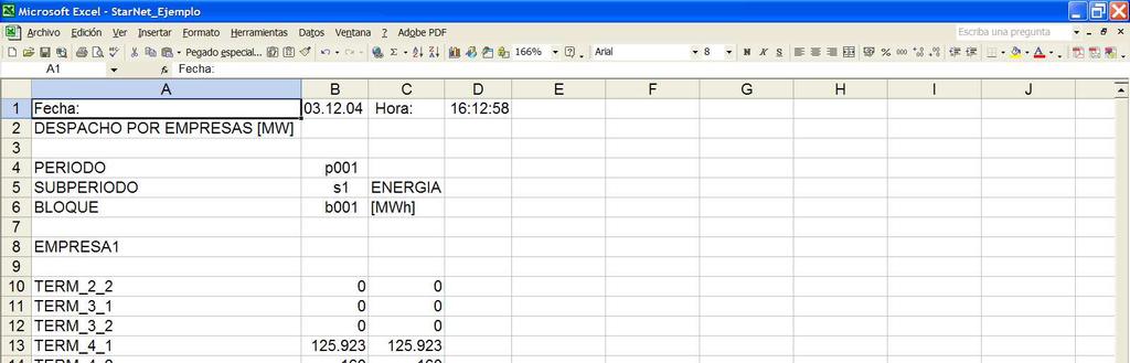
40 StarNet/RD (ix) 42

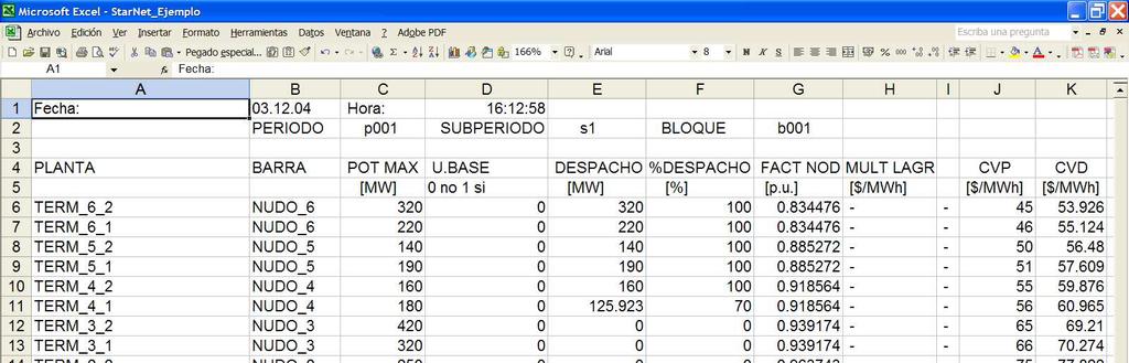
41 StarNet/RD (x) 43

42 CHOPIN G. Latorre, J.I. Perez-Arriaga CHOPIN, A HEURISTIC MODEL FOR LONG TERM TRANSMISSION EXPANSION PLANNIG IEEE Transactions on Power System, Vol. 9, No. 4, November

43 PLAER de Dios, R., Sáiz, A., Melsión, J.L. y Bassy, A., PLAER. Strategic Transmission Network Planning. 11TH Power System Computation Conference, August

44 PERLA J.F. Alonso, A. Sáiz, L. Martín G. Latorre, A. Ramos, I.J. Pérez-Arriaga PERLA: An Optimization Model for Long Term Expansion Planning of Electric Power Transmission Networks IIT January 1991 ( A.pdf) 46

45 SIMUPLUS (i) Determine incremental investment needs in transmission network for the medium term in electricity markets Scenario Sampling: Bids & Failures Market Clearing Procedure: MO model Transmission Adequacy: SO model Transmission Investment Results P. Sánchez-Martín, A. Ramos, J.F. Alonso Probabilistic mid-term transmission planning in a liberalized market IEEE Transactions on Power Systems 20 (4): Nov 2005 ( WRS pdf) Stop Criterion reached? Yes Multiobjective Investment Analysis No 47

46 SIMUPLUS (ii) 1. Monte Carlo sampling: Demand bids and generation offers Units and circuits availability Hydro and wind generation 2. Single node market clearing Losses included as additional demand 3. Network constraint evaluation penalizing deviations with respect to market clearing DC load flow, flow limits, losses N-1 contingencies 4. Determine sensitivities (derivative of the objective function with respect to investment): Improvement in existing circuits New circuit expansion 48

47 SIMUPLUS (iii) 5. Investment multi-attribute analysis Weigh sensitivities average, confidence interval, validity range, investment needs, environmental impact, etc. Investment selection 6. Repeat all the process 49

48 SIMUPLUS (iv) Spanish Iterative Investment Ranking Stag e Candidates Sensitivity mean [M$/M$] Confidence interval [%] No circuit is added (initial stage) Validity range [MW] Multiattribute value Circuit is added Circuits and are added Circuits , and are added Circuits , , and are added No more circuits are added 623 nodes and 1021 circuits, 165 thermal units and 76 hydro units. 12 network expansion alternatives. Sampling of 100 scenarios in each stage and Deviation and Overload Decrement [%] obtain the 3 best alternatives. Deviation Penalization Overload Penalization Operation Cost Cumulative Circuits Operation Cost Decrement[%]

49 Summary Where to use a composite reliability model Some characteristics to be considered into this model Mathematical techniques used to solve the model Some real applications 51

50 Contact: EMIN: International Master in Economics and Management of Network Industries Contact: Alberto Aguilera 23, E Madrid - Tel: Fax: