CHEM-E5225 :Electron Microscopy Imaging II

Transcription

1 CHEM-E5225 :Electron Microscopy Imaging II D.B. Williams, C.B. Carter, Transmission Electron Microscopy: A Textbook for Materials Science, Springer Science & Business Media, Z. Luo, A Practical Guide to Transmission Electron Microscopy, Volume II: Advanced Microscopy, Momentum Press, B. Fultz, J.M. Howe, Transmission Electron Microscopy and Diffractometry of Materials, Springer Science & Business Media,

2 Outline Planar Defects Image strain field WBDF microscopy HRTEM

3 Planar Defects - Internal Interface

4 Translations and Rotations Translation Boundary, RB. R(r), is zero. Grain boundary, GB. Any values of R(r), n and are allowed. Phase boundary, PB. As for a GB, but the chemistry and/or structure of the regions can differ. Surface. A special case of PB where one phase is vacuum or gas.

5 Why Do Translations Produce Contrast? Planar defects are seen when 0 ( 2n ). g is operation vector = 0 or = 2n g R = 0 or integer Defect is invisible Brent Fultz, James M. Howe, Transmission Electron Microscopy and Diffractometry of Materials, Springer Verlag Berlin Heidelberg, /

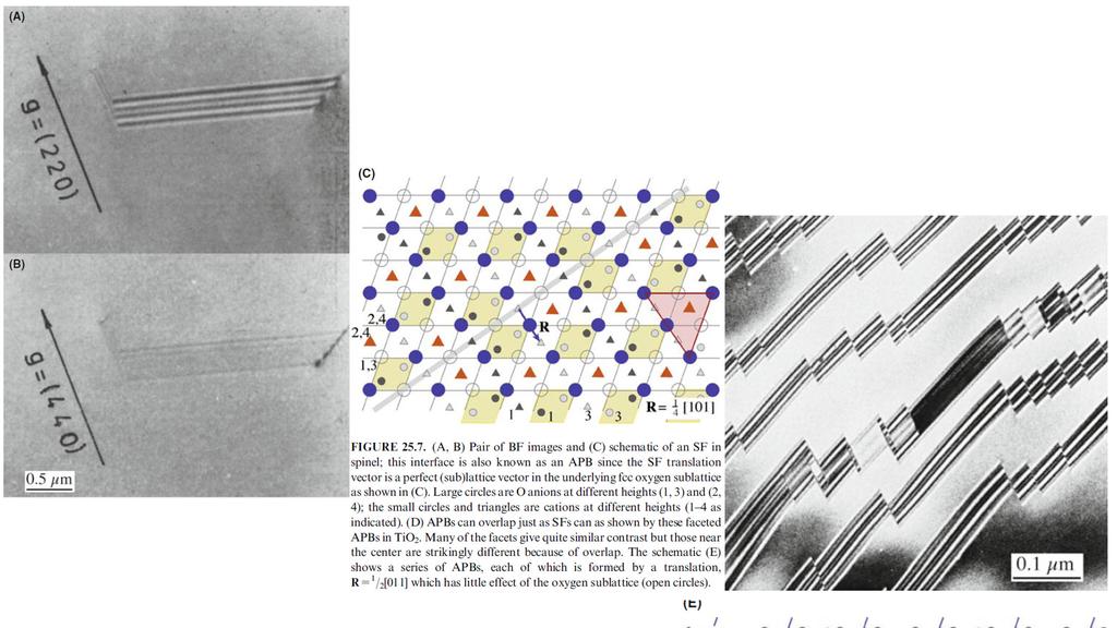
6 Why stacking faults are invisible when g R = interger 2_dec2010.pdf kiel.de/matwis/amat/def_en/index.html

7 Stacking Faults in FCC Materials Stacking faults bounds by 1/6 <112> Shockley partial dislocations Intrinsic fault: remove a layer Extrinsic fault: insert a layer Stacking faults bounds by 1/3 <111> Frank partial dislocations For a FCC the translations are then directly related to the lattice parameter: R is either 1/6 <112> or 1/3 <111> The J. Chemical Physics 130, (2009); doi: /

8 Stacking faults -FCC Faults visible n= 0, 1, 2 Faults invisible

9 Invisibility Criterion: g R = 0,1,2. Type A = Type B = + Invisible: g.r = 0 equal g.r =1 or integer =2n Visible: g.r =1/3 equal g.r = 4/3, g.r is 0 to 1.

10 Some rules for interpreting the contrast In the image, as seen on the screen or on a print, the fringe corresponding to the top surface (T) is white in BF if g R is > 0 and black if g R <0. Using the same strong hkl reflection for BF and DF imaging, the fringe from the bottom (B) of the fault will be complementary whereas the fringe from the top (T) will be the same in both the BF and DF. The central fringe fade away as the thickness increases. Displace aperture instead of CDF for using same hkl for both BF and DF.

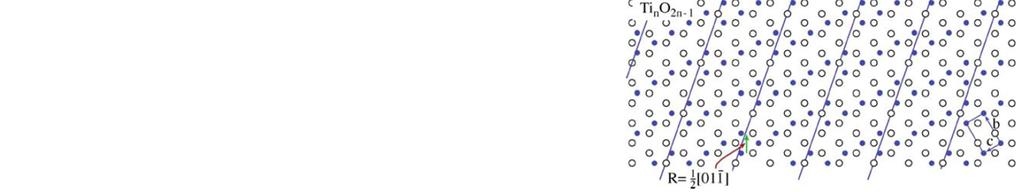
11 Other Translations: Fringes - =

12 Phase Boundaries Rotation Boundaries

13 Imaging Strain Fields

14 Why image Strain Field The direction and magnitude of the Burgers vector, b, which is normal to the hkl diffraction planes. The line direction, u (a vector), and therefore, the character of the dislocations (edge, screw, or mixed). The glide plane: the plane that contains both b and u.

15 Howie-Whelan Equations Assumption: two beam treatment, linear elasticity, column approximation. The contrast of the defects will depend on both s and g. g R contrast is used when R has a single value, s R contrast is used when R is a continuously varying function of z, which in turn is associated with g dr/dz.

16 The displacement field R The displacement field in an isotropic solid for the general, or mixed, case e.g. b is not parallel to u:

17 Contrast from a Single Dislocation Screw dislocation: b e = 0 and b x u = 0. g R is proportional to g b. Pure edge dislocation: b = b e. g R involves two terms g b and g b x u.

18 Dislocations contrast g b criterial Edge dislocation : b u Screw dislocation: b u Dislocation glide plane: b u 1. Screw dislocation invisible criterion: g b = 0 also applied to edge dislocation if g u 2. Pure edge dislocation invisible criterion: g b = 0 residual contrast criterion g (b u) = 0 1. Tilt sample to find u. 2. To find g1 and g2 operations for dislocation invisible: b (g1 g2)

19 Contrast from a Single Dislocation Experimental point: you usually set s to be greater than 0 for g when imaging a dislocation in two-beam conditions. Then the dislocation can appear dark against a bright background in a BF image. Identify two reflections g 1 and g 2 for which g b = 0, then g 1 x g 2 is parallel to b. * In practice, when g.b <1/3, contrast is very weak already, especially for partial dislocations. How to identify u?

20 Screw dislocation Edge dislocation Brent Fultz, James M. Howe, Transmission Electron Microscopy and Diffractometry of Materials, Springer Verlag Berlin Heidelberg, /

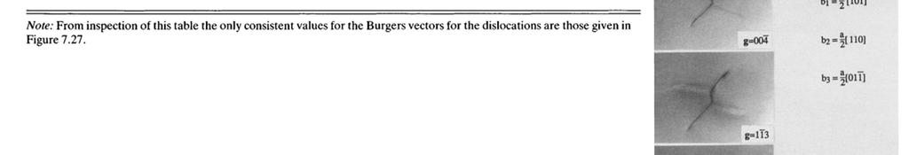
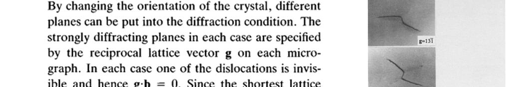
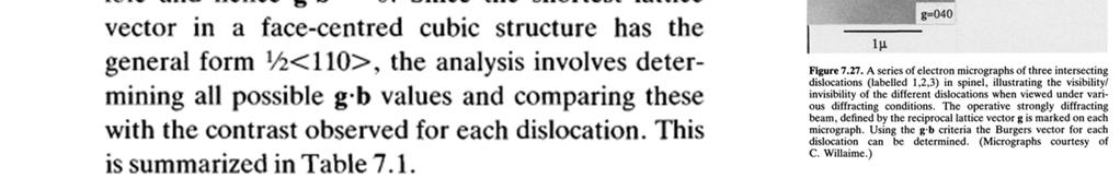
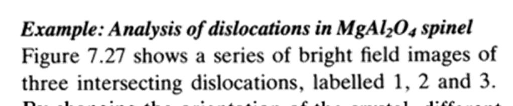
21 Example of determination of b From book: An Introduction to Mineral Sciences

22 Dislocation Nodes and Networks Dislocation Loops

23 Dislocation dipoles Dipoles can be thought of as loops which are so elongated that they look like a pair of single dislocations of opposite Burgers vector, lying on parallel glide planes. As a result, they are best recognized by their inside-outside contrast.

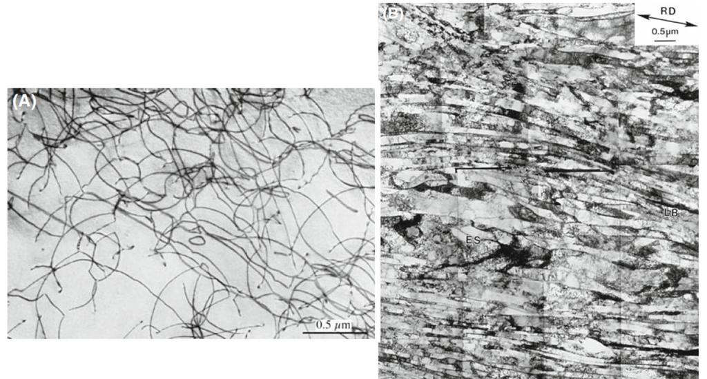
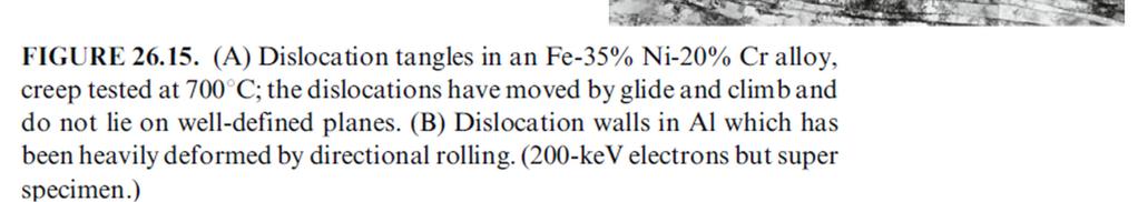
24 Dislocation Pairs, Arrays, and Tangles

25 Surface Effects Dislocation strain fields are long range, but we often assign them a cut-off radius of 50nm. However the specimen thickness might only be 50nm or less. The surface can affect the strain field of the dislocation, and vice versa.

26 Dislocations and Interfaces Misfit dislocations accommodate the different in lattice parameter between two well-aligned crystalline. Transformation dislocations are the dislocations that move to create a change in orientation or phase.

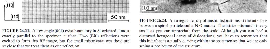
27 Dislocations and Interfaces

28 Volume Defects and Particls

29 Weak-Beam Dark-Field Microscopy

30 Weak-Beam Dark-Field image

31 Intensity in WBDF Images In a perfect crystal the intensity of the diffracted beam in two beam condition: In the WB technique we increase s to about 0.2 nm -1 so as to increase s eff.

32 How To Do WBDF CDF with small objective aperture on optimized thickness

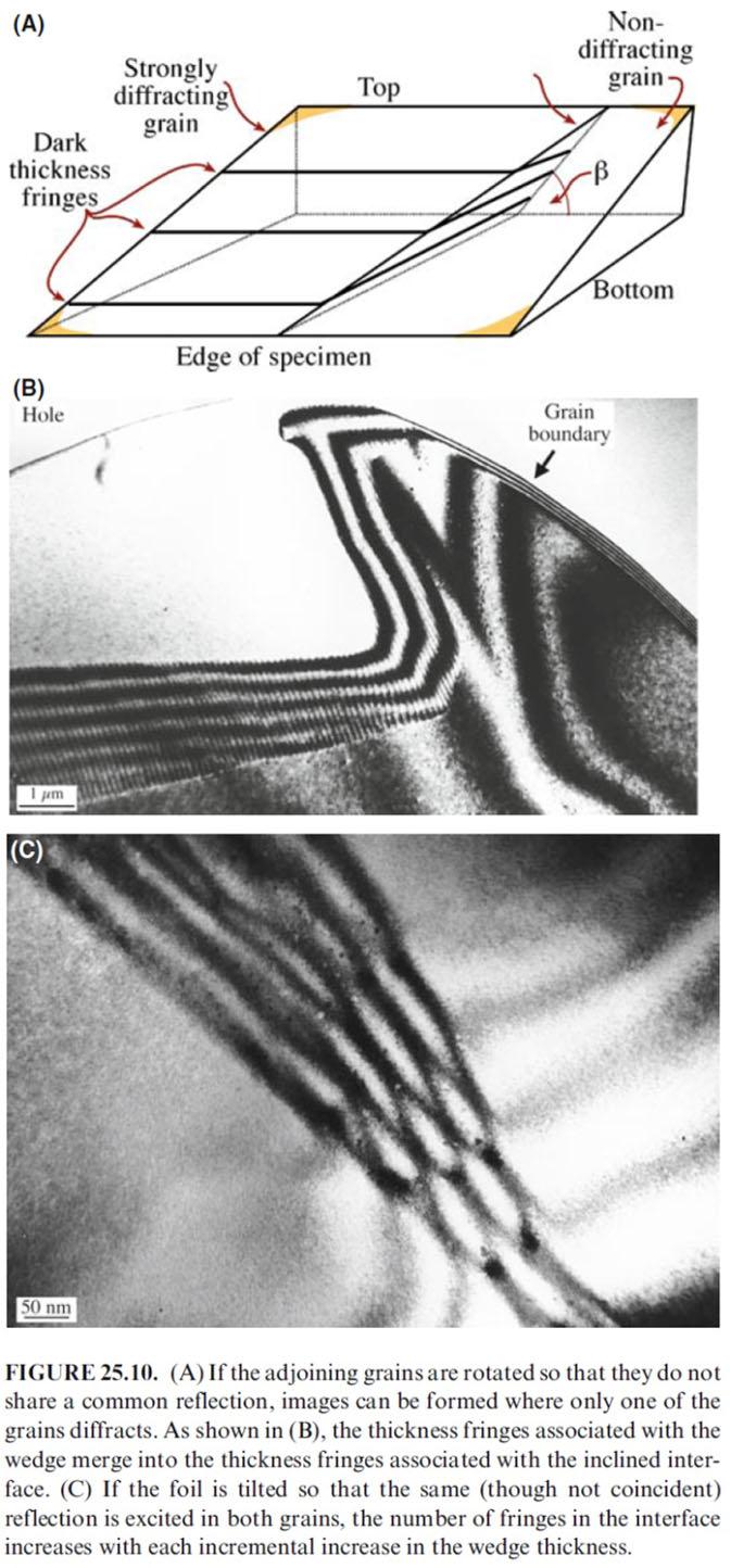
33 Thickness Fringes in Weak-Beam Images

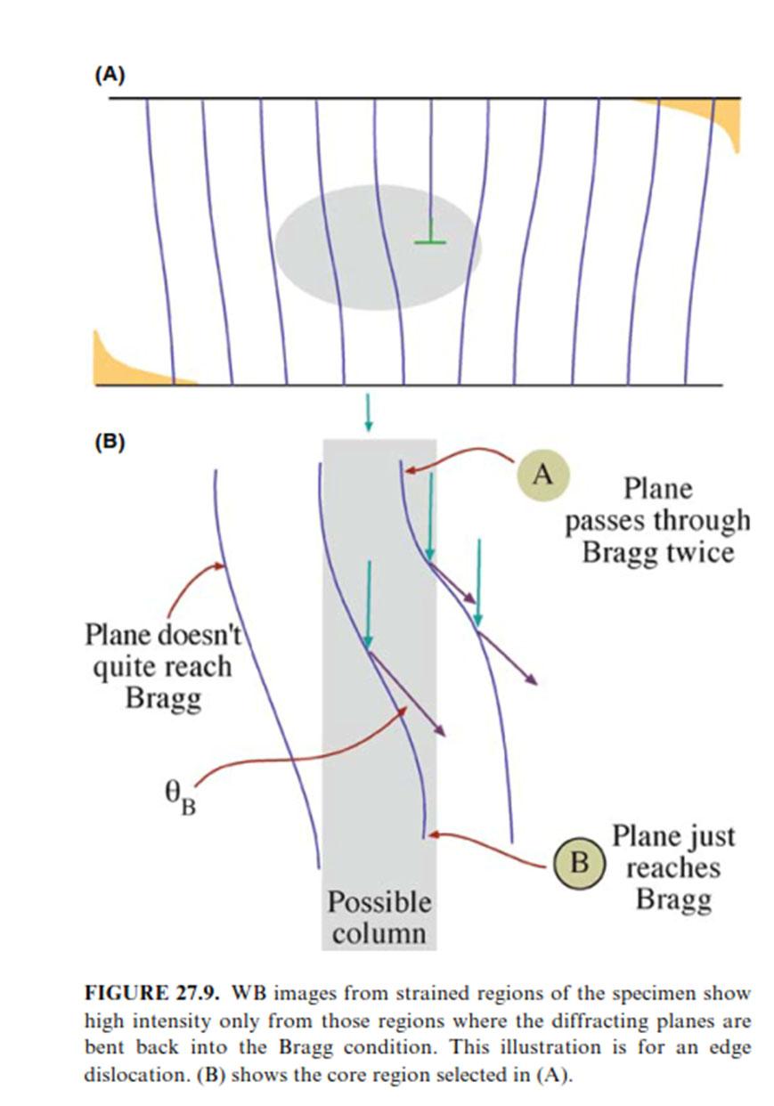
34 Imaging Strain Field

35 Weak-Beam Images of Dissociated Dislocations In WB image with g b T = 2, each of the partial dislocations will generally give rise to a single peak in the image which is close to the dislocation core. You can relate the separation of the peaks in the image to the separation of the partial dislocations.

36 High-Resolution TEM

37 The Origin of Lattice Fringes Two beam condition, interference of direction beam and diffracted beam. The intensity of phase contrast is a sinusoidal oscillation normal to g, with a periodicity that depends on s and t. This simple analysis shows that the location of a fringe does not necessarily correspond to the location of a lattice plane.

38 Some Practical Aspects of Lattice Fringes s = 0, hkl // optic axis s 0; hkl edge on If s 0 If s is not zero, then the fringes will shift by an amount which depends on both the magnitude of s and the value of t, but the periodicity will not change noticeably. The fringe periodicity is the same as the spacing of the planes which give rise to g. this result holds wherever s = 0 no matter how 0 and g are located relative to the optic axis, even if the diffraction planes are not parallel to the optic axis. We expect this s dependence to affect the image when the foil bends slightly, as is often the case for thin specimens. We also expect to see thickness variations in many-beam images, since s may be non-zero for all of the beams; s may also vary from beam to beam.

39 Image Real Structure Reality Ideal

40 High Resolution Transmission Electron Microscopy

41 Exit wave function Phase shift over a thickness t is: At the sample exit, the wave function becomes: For very thin crystals, (xy) 1, following weak phase object approximation (WPOA):

42 Contrast Transfer Function H(u) The wave function on the back focal plane is mathematically a Fourier transformation (FT) of the wave function 1 (xy) but multiplied by a contrast transfer function (CTF), H(u), Where u is a reciprocal vector with a length of u. H(u) includes the following components: Each point in the specimen plane is transformed into an extended region (or disk) in the final image. Each point in the final image has contributions from many points in the specimen.

43 Contrast Transfer Function H(u) (a) Aperture Function A(u): (b) Envelope Function E(u): includes chromatic aberration envelope function E c (u) and spatial coherence envelop function E s (u):

44 Contrast Transfer Function H(u) (c) Aberration Function B(u) : - Aberration function Phase shift by the spherical aberration: Phase shift by the defocus f Scherzer deduced that the optimum defocus condition: Scherzer defocus:

45 Contrast Transfer Function - wikipedia Contrast Transfer Function (CTF) mathematically describes how aberrations in a TEM modify the image of a sample. This CTF sets the resolution of HRTEM, also known as phase contrast TEM. The function exists in the spatial frequency domain, or k space Whenever the function is equal to zero, that means there is no transmittance, or no phase signal is incorporated into the real space image The first time the function crosses the x axis is called the point resolution To maximize phase signal, it is generally better to use imaging conditions that push the point resolution to higher spatial frequencies When the function is negative, that represents positive phase contrast, leading to a bright background, with dark atomic features Every time the CTF crosses the x axis, there is an inversion in contrast Accordingly, past the point resolution of the microscope the phase information is not directly interpretable, and must be modeled via computer simulation

46 Contrast Transfer Function H(u) For 200kV TEM, = nm, C s = 0.8mm, f sch = 51.74nm Under the Scherzer defocus condition, the sin curve exhibit a wide flat range with the valley value of 1. This range can transfer the contrast with the same sign (all negative) and with the highest contrast (at or near 1, far away from zero.) The first zero point, u sch, is the limit to reveal details that is the resolution of the microscope r sch.

47 Contrast Transfer Function H(u)

48 Image Formation of image plane Image at image plane is a simple mathematcial Foourier transformation of the wave function (u) from the reciprocal space to the real space: Under optimum condition < 1, and the atoms show black contrast. = /( E) interaction constant : defocus due to chromatic aberration

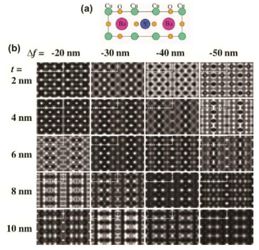
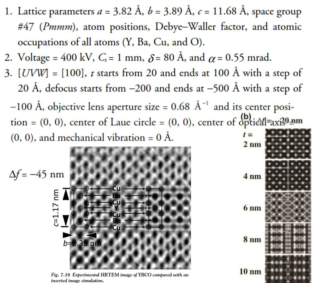
49 Image interpretation and simulation 400kV

50 Some Difficulties In Using An FEG A cold FEG has a small emitter area and Schotty emitter has a source diameter 10 times greater, but with a decrease in spatial coherence and a larger energy spread. Correcting astigmatism is very tricky. Need on-line processing (live FFT). Focal series of image are a challenge with a large range of f values. Image delocalization occurs when detail in the image is displaced relative to its true location in the specimen.

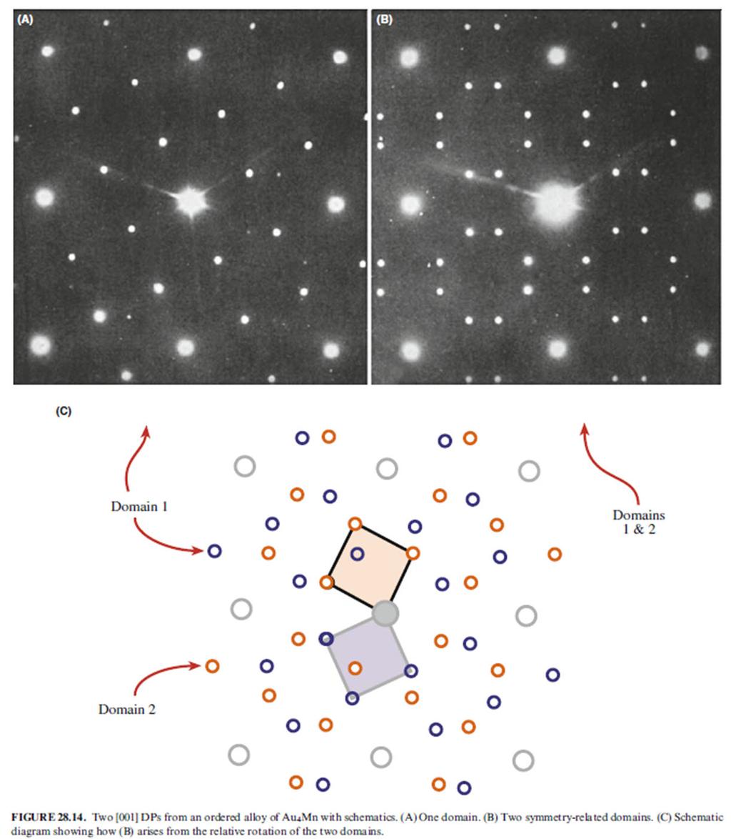
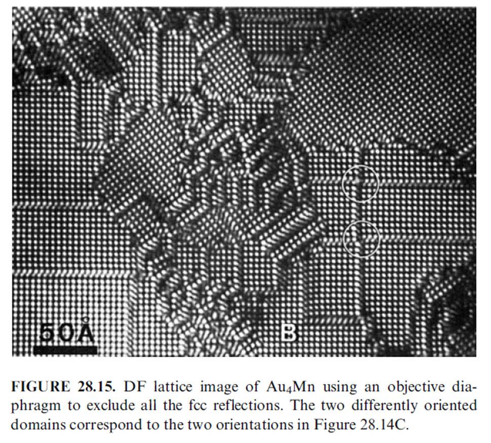
51 Selectively Imaging Sublattices

52 Interfaces And Surfaces The fundamental requirement is that the interface plane must be parallel to the electron beam.

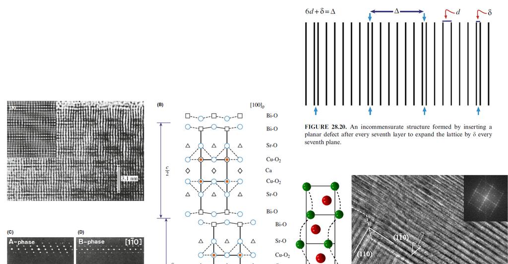
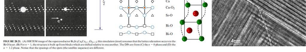
53 Incommensurate Structures

54 Quasicryatals HRTEM excels when materials are ordered on a local scale. For HRTEM, we need the atoms to align in columns because this is a projection technique, but the distribution along the column is not so critical. And we can t determine it without tilting to another projection in the perfect crystal. SAD and HRTEM should be used in a complementary fashion.

55 Single Atoms Observation by Parsons et al. with dedicated STEM: uranium atoms in molecule matrix.

56 Home works