Experimental Procedure. Lab 402

Transcription

1 Experimental Procedure Lab 402

2 Procedure Overview Cyclohexane is the solvent selected for this experiment although other solvents may be just as effective for the determination of the molar mass of a solute. The freezing points of cyclohexane and a cyclohexane solution are determined from plots of temperature versus time. The mass of the solute us measured before it is dissolved in a known mass of cyclohexane. You ll use the cyclohexane throughout the experiment. Your TA will issue you about 1 g of unknown solute. Record the unknown number of the solute on the Report Sheet.

3 The cooling curve to be plotted in PART A.4 can be established by using a thermal probe that is connected directly to computer with the appropriate software. Trial # and Run # Solvent and Solute On Manual On Computer Solvent Unknown solid PART A Run 1 Test tube 1 Cyclohexane 12 ml PART B.1, B.3 Trial 1 Run 2 Test tube 2 Cyclohexane 12 ml g PART B.4 Trial 2 Run 3 Additional g PART B.5 Trial 3 Run 4 Additional g

4 Set-up of computer and probe a. Plug both an interface and a computer to main power. b. Connect a temperature probe to channel 1 of the Vernier computer interface. c. Connect the interface to the computer with the proper cable.

5 d. Start the Logger Pro program by double clicking on the desktop. e. Open the file 04 Freezing Point from the Advanced Chemistry with Vernier folder. We will utilize a template for this experiment.

6

7 [Experiment] -> [Data Collection] Choose and Input {time based/ 300 seconds/ 2 seconds/sample}

8

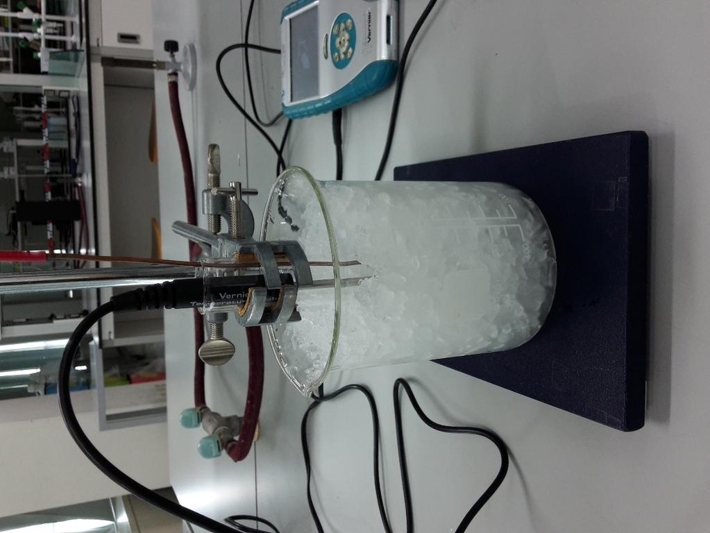
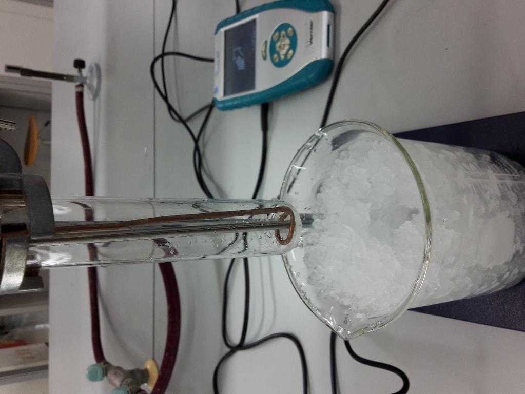
9 A. Freezing Point of Cyclohexane (solvent) 1. Prepare the ice-water bath Assemble the apparatus shown in below. Obtain a digital thermometer, mount it with a thermometer clamp to the ring stand, and position the thermometer in the test tube.

10

11

12 2. Prepare the cyclohexane 1) Determine the mass (±0.01 g) of a clean, dry 150-mm test tube in a 250-mL beaker. 2) Add approximately 12 ml of cyclohexane to the test tube. 3) Place the test tube containing the cyclohexane into the ice-salt bath. [Prepare the bath in advance as follows; add 65 g of NaCl into the bath with ice and mix it well (Ice : NaCl = 3 : 1, -20 o C).] 4) Secure the test tube with a utility clamp. Insert the thermometer probe and a wire stirrer into the test tube. 5) Secure the thermometer so that the thermal sensor is completely submerged into the cyclohexane.

13 3. Freezing Temperature Determination (RUN 1) 1) While stirring with the wire stirrer, click Collect to begin the data collection. 2) The temperature remains virtually constant at the freezing point until the solidification is complete. 3) Continue collecting data until the temperature begins to drop again. 4) With a very slight up and down motion of the wire stirrer, continuously stir the solvent for the three-minute duration of the experiment. (*Continuous stirring of the cyclohexane solvent is necessary to avoid supercooling and uneven cooling. Thermometers are not stirring rods!)

14 Click [Collect]

15 [Experiment] -> [Store Latest Run]

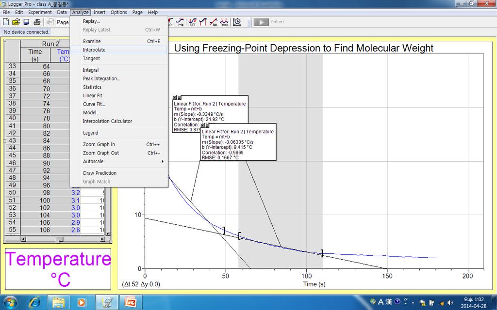
16 The freezing temperature can be determined by finding the mean temperature in the portion of the graph with nearly constant temperature. a. Move the mouse pointer to the beginning of the graph s flat part. Press the mouse button and hold it down as you drag across the flat part of the curve, selecting only the points in plateau. b. Click the Statistics button. c. The mean temperature value for the selected data is listed in the statistics box on the graph. d. Record this value on your Result Summary as the freezing temperature of pure cyclohexane. e. Click on the upper-left corner of the statistics box to remove it from the graph.

17 Selection of the points in plateau ->[Analyze] -> [Statistics]

18 B. Freezing Point of Cyclohexane plus Unknown Solute Three freezing point trials for the cyclohexane solution are to be completed. Successive amounts of unknown sample are added to the cyclohexane in PARTs B.4 and B.5

19 1. Measure the mass of solvent and solid solute 1) Dry the outside of the test tube containing the cyclohexane and measure its mass in the same 250-mL beaker. 2) On weighing paper, tare the mass of g of unknown solid solute and record. 3) Quantitatively transfer the solute the cyclohexane in the 150- mm test tube. (*All of the solute must dissolve-no solute should adhere to the test tube wall.)

20 2. Record data for the freezing point of solution Collect data for determination of the freezing point of this solution in the same way as that of the solvent. 3. Plot the data on the same graph (RUN 2, Trial 1) You can see the graph of the temperature versus time data on the same graph (and same coordinates) as those for the pure cyclohexane (PART A.4) From the Experiment menu, choose Store Latest Run.

21 4. Repeat with additional solute (RUN 3, Trial 2) Remove the test tube and solution from the ice-water bath. Add an additional g of unknown solid solute using procedure as in PART B.1. From the Experiment menu, choose Store Latest Run. Again plot the temperature versus time data on the same screen PART B.2 and B.3. The total mass of solute in solution is the sum from the first and second trials.

22 5. Again. Repeat with additional solute (Run 4, Trial 3) Repeat PART B.4 with an additional g of unknown solid solute, using the same procedure as in PART B.1. From the Experiment menu, choose Store Latest Run. Again plot the temperature versus time data on the same graph PART B.2-4. The total mass of solute in solution is the sum for the masses added in PARTs B.1, B.4 and B.5. You now should have four plots on the same graph.

23 C. Freezing Temperature Determination of Run2 (Trial1), Run3 (Trial 2), and Run 4 (Trial 3) The freezing temperature of the solution can be determined by finding the temperature at which the mixture initially started to freeze. 1. To obtain the freezing temperature of Run 2 (Trial 1) a. To hide the curve of your Run 1, run 3, run 4 and Latest Run, click the Temperature y-axis label of the graph and choose More from the dropdown list. b. Uncheck Temperature boxes in each Run, 1, 3, 4 & Latest Run and click OK.

24 Click the Temperature y-axis label of the graph and choose More.

25 Uncheck Temperature boxes in each Run, 1, 3, 4 and Latest Run and click OK..

26 c. Click and drag the mouse to highlight the initial part of the cooling curve where the temperature decreases rapidly (before freezing occurred). d. Click on the Linear Regression button. e. Now click and drag the mouse over the next linear region of the curve (the gently sloping section of the curve where freezing took place). f. Click the Linear Regression button again. The graph should now have two regression lines displayed. g. Choose Interpolate from the Analyze menu. Move the cursor to the point of intersection of the two lines; you will know if the cursor is over the intersection when the temperature readings displayed in the Interpolate box are the same. This is the freezing point of the solution. h. Record the freezing point in the Result Summary.

27 The cooling curve for the solution does not reach a plateau but continues to decrease slowly as the solvent freezes out of solution. Its freezing point is determined at the intersection of two straight lines drawn through the data points above and below the freezing point.

28

29

30

31 2. To get the freezing temperature of Run 3 (Trial 2) a. Follow the same steps like PART C.1. to determine the freezing point of the solution, Run 3 b. Record the freezing point in the Result Summary. 3. To get the freezing temperature of Latest Run (Trial 3) a. Follow the same steps like PART C.1. to determine the freezing point of the solution, Run 3 b. Record the freezing point in the Result Summary.

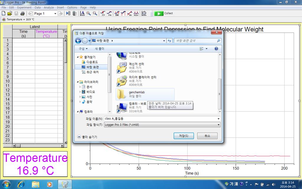
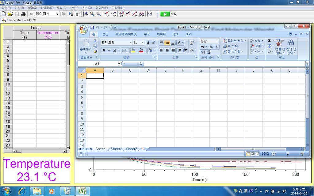
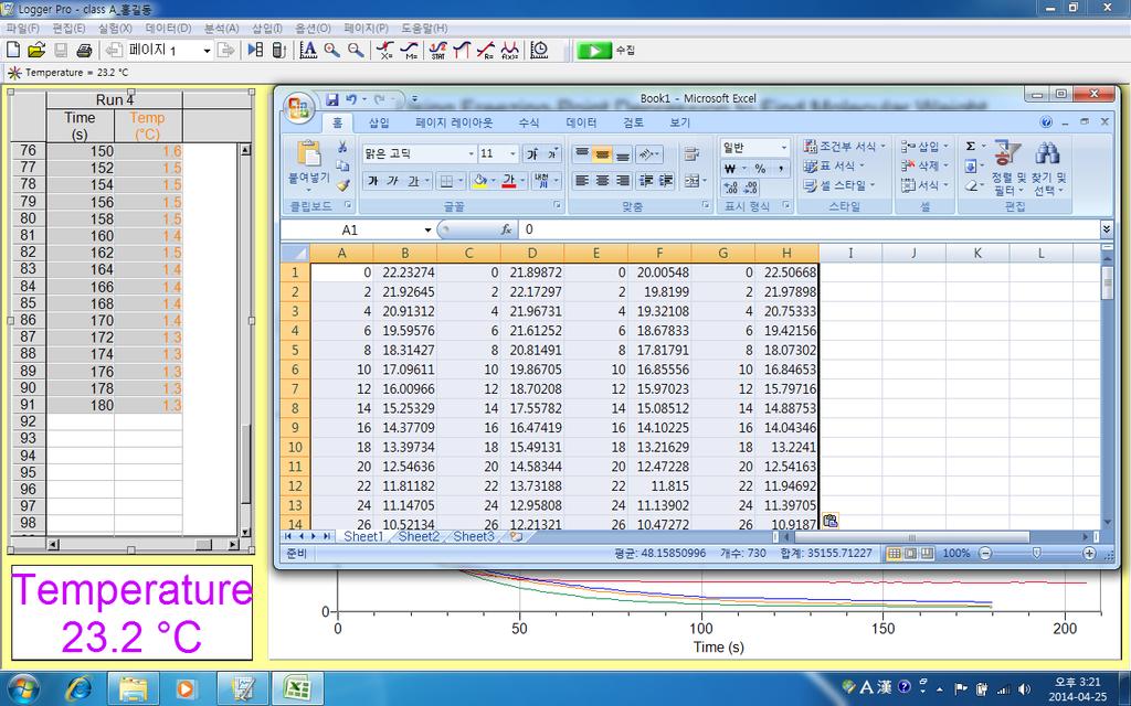
32 SAVE AS To save the current data file, choose SAVE AS from the File menu under a different name. Store the file with a file name, [class-name] in a folder of GENCHEM_EXP8 on the desktop. Logger Pro and newer files are saved with cmbl extension. Copy and Paste into Microsoft Excel 1. Select the data in the data table. You can select data by clicking and dragging the mouse pointer across ranges of cells. 2. Choose Copy from the Edit menu to copy the data. 3. Start Excel and open the document into which you want to paste the data. 4. In Excel, click on the cell that will be upper left corner of the data region, then Paste from the Edit menu. 5. Save the Excel file with proper name.

33

34

35

36

37 You must send the Excel file to you and your TA via after logging into wireless networking, KAIST Wireless Lan system. (To do that, you first need to get a ID and password at to access KAIST Wireless Lan program.)

38 Graphical Analysis of Data Use the Excel program to create four separate graphs of Temperature versus Time for the pure solvent and the three solutions from your data. Each graph should have an appropriate title and labeled axes with an appropriate scale. Add two trendlines to the data points of each graph. Extrapolate the two trendlines towards each other until they intersect. The temperature at this point of intersection is the solvent freezing point and should be clearly shown on each graph. Submit the graphs and results with the lab report. (Attach a separate sheet of calculations and graphs if necessary).

39 D. Calculations 1. From the plotted data, determine ΔT f for Trial 1, Trial 2, and Trial 3. Refer to the plotted cooling curves (see Figure 14.3) 2. From k f (Table 14.1), the mass (in kg) of the cyclohexane, and the measured ΔT f calculate the moles of solute for each trial. See equations 14.1 and Determine the molar mass of the solute for each trial (remember the mass of the solute for each trial is different). 4. What is the average molar mass of your unknown solute? 1. Calculate the standard deviation and the relative standard deviation (% RSD) for the molar mass of the solute.

40 CLEANUP: Safety store and return the thermometer. Rinse the test tube once with acetone; discard the rinse in the Waste Organic Liquids container. Clay triangle DISPOSAL: Dispose of the waste cyclohexane and cyclohexane solution in the Waste Organic Liquids container. Bunsen burner