CHAPTER 4 DIFFUSIVITY AND MECHANISM

Transcription

1 68 CHAPTER 4 DIFFUSIVITY AND MECHANISM 4.1 INTRODUCTION The various elements present in the alloys taken for DB joining diffuse in varying amounts. The diffusivity of elements into an alloy depends on parameters such as temperature, pressure and time. Apart from the above said parameters, the surface finish is also an important parameter to obtain even diffusion. Therefore, surface finish to the highest degree is required to obtain even diffusion of atoms, which creates a solid solution and compounds of the two metals in the zone of contact. The void closure mechanism is studied, as heavy pressures are applied prior to bonding at about 750 C to break the surface asperities to obtain smooth surface. 4.2 DIFFUSION MECHANISM Substitution Diffusion Mechanism A solute atom occupies lattice site of a solvent atom. This type of diffusion mechanism is known as substitution diffusion. The Figure 4.1 reveals a solute atom substituting a solvent atom. In adition, diffusion takes place through the movement of point defects.

2 69 Figure 4.1 Diagram showing substitution and interstitial diffusion mechanism. Addition of an impurity element in a pure substance results in substitution diffusion.the presence of different types of defects give rise to different mechanisms of diffusion Vacancy Mechanism Vacancy is a point defect in a crystal lattice. An atom jumps to occupy a vacant position when it is subjected to higher temperature. This mechanism is called vacancy mechanism as reported by Krishtal (1973). The displaced atom creates a vacant site that promotes further diffusion. Gruzin (1960) explained laws of diffusion and distribution of various elements in ferrous material. In Figure 4.2 mode of vacancy mechanism is shown.

3 70 Figure 4.2 Diagram showing vacancy diffusion mechanism Interstitial Diffusion Mechanism An interstitial atom or an atom of an element moves to interstitial void position effecting interstitial diffusion mechanism. Placing an atom at the interstitial site distorts the crystal lattice. This type of diffusion mechanism is possible only when the diffusing atom is smaller than the parent element in the lattice. Diffusion of interstitial elements such as H, C, N and O in metals is an example of this mechanism. 4.3 DIFFUSION COEFFICIENT VALUES Low-Carbon Steel Grade AISI 1018 with AISI 304L with Interlayer Fick s second law for unidirectional flow under steady state conditions is given below C t x D C x (4.1) After measuring the concentration of an element (C x ) at a distance x from the interface, the Fick s second law is rewritten as given below.

4 71 C t x D 2 C x x 2 (4.2) The solution to this equation is as follows: C ( x, t) A Berf 2 x Dt (4.3) A C C C2 C1, B 2 (4.4) where C 1 and C 2 are the initial concentrations of the element under study in both sides of the diffusion couple, x is the distance from the interface, t is the bonding time and D is diffusion coefficient as mentioned by Raghavan (2004). Diffusion of various elements from one plane to another plane in a diffusion couple is illustrated in the Figure 4.3. Figure 4.3 A model showing diffusion across a diffusion couple.

5 72 The elemental concentration and distance from the interface on either side of the base metals and the interlayer was measured using SEM and EDAX. Based on these measurements, the diffusion coefficients and the ratio between D Cr and D Ni values in the interface between low carbon steel and interlayer AISI 304L were calculated and shown in Table 4.1. A graph drawn between homologous temperatures of AISI 1018 and diffusion coefficient values is shown in Figure 4.4. Table 4.1 Diffusion coefficients (D) of various elements (into AISI 1018 steel). Process parameters C/MPa/Min D Cr m 2 /s D Ni m 2 /s D Mn m 2 /s D Cr /D Ni D Cr /D Mn D Ni /D Mn 850,10, ,10, ,10, Figure 4.4 Homologous temperatures of AISI 1018 steel vs. Diffusion coefficients.

6 DSS SAE 2205 Bonded with AISI 1035 Steel The SEM and EDAX analyses were performed to measure concentration of various elements across the interface at various distances. Based on these measurements, the diffusion coefficient values for various elements such as Cr, Ni, Si, Cu, Mo and Mn (diffusion from SAE 2205 with AISI 1035 took place) were determined and shown in Table 4.2. Kundu et al (2011) presented the determination of the activation energy Q and k o by plotting 1/T vs. ln(x) 2 kt (4.5) k o Q RT k exp (4.6) Where X is the thickness of the reaction layer, t is the time of bonding, T is the bonding temperature (kelvin), k is the growth velocity in m 2 /s, and k o is the growth constant and Q is the activation energy in KJ/mol.K. The k term is equated to diffusion coefficient and k o is equated to pre-exponential constant in the present study. The distance X is determined from the equation (4.5) by substituting D and t in place of k and t. A graph is plotted as described above adopting the method proposed in the work of Kundu et al (2011). The slope of the linear plot gives the activation energy Q and Y -intercept gives the pre-exponential constant D o. However, another method of plotting graph 1/T vs. ln (D) can be used to obtain Q and D o values. When second method was adopted to determine D o and Q values, those values were very less. Because of this, the first method proposed by Kundu et al (2011) was used for the estimation of D o and Q values in this study.

7 74 Table 4.2 Diffusion coefficients (D) of various elements (into AISI 1035 steel). Process parameters C/MPa/Min. Diffusion coefficient values in m 2 /s Cr Ni Si Cu Mo Mn 850,30, ,20, ,30, ,20, ,20, ,30, ,20, Note: D values for Si, Cu and Mn were not determined for all cases because the calculated error function values were not within limit. The pre-exponential constant (D o ) and activation energy (Q) for various elements in AISI 1035 steel are shown in Table 4.3. The graphs shown in Figure 4.5 (a), (b) and (c), drawn between 1/T and ln(x) gives the pre-exponential constant and activation energy D o and Q values, respectively. A graph drawn between homologous temperatures of AISI 1035 and diffusion coefficient values is shown in Figure 4.6. Table 4.3 Pre-exponential constant (D o ) and activation energy of various elements. Group I II Process parameters o C/MPa/Min. 900,20,90 950,20,90 975,20,90 850,30,90 900,30,90 950,30,90 D o m 2 /s Cr Ni Mo QKJ/ D o QKJ/ D o Mol. K m 2 /s Mol. K m 2 /s QKJ/ Mol. K

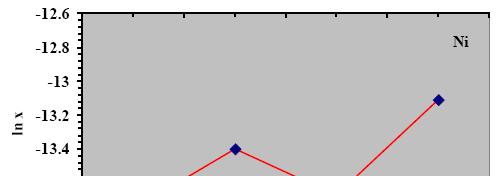
8 75 Figure 4.5 Graphical plot between distance vs. temperature: (a) for Cr, (b) for Ni and (c) for Mo. Figure 4.6 The Homologous temperatures of AISI 1035 steel vs. Diffusion coefficients.

9 76 Table 4.4 Ratios between D values of various elements (SAE 2205 with AISI 1035). Process parameters o C/MPa/Min. D Cr /D Ni D Cr /D MO D Cr /D Si D Cr /D Mn D Cr /D Cu D Ni /D Mo 850,30, ,20, ,30, ,20,60 * * - - * ,20, ,30, ,20, Note: *-The determined values are highly erratic and hence, they are not presented in the Table 4.4. The ratios between diffusion coefficient values of various elements are shown in Table TI-6AL-4V Bonded with AISI 304L The EDAX examination was performed at various points to estimate elemental concentration. The diffusion coefficient values D were determined as described in section The activation energy Q and preexponential constant D o values were determined as explained in the section The graphs shown in Figure 4.7 (a), (b) and (c), drawn between 1/T and ln(x) gives tha pre-exponential constant and activation energy D o and Q values, respectively. Also, Figures 4.8 (a) and (b) are used to estimate D o and Q values of Ti and V, respectively. A graph drawn between homologous temperatures of Ti-6Al-4V and diffusion coefficient values is shown in Figure 4.9. In addition, a graph

10 77 drawn between homologous temperatures of AISI 304L and diffusion coefficient values is shown in Figure Table 4.5 Diffusion coefficients (D) of various elements. Process parameters ºC/MPa/ Min. Diffusion of elements into Ti-6Al- 4V Diffusion of elements into AISI 304L D Fe D Mn D Ni D Ti D Al D V 875, 8, , 4, , 8, , 4, Table 4.6 Pre-exponential constant (D o ) and activation energy of various elements. Process parameters o C/MPa/Min. D o m 2 /s Fe Mn Ni Ti V Q KJ/ Mol. K D o Q KJ/ D o m 2 /s Mol. K m 2 /s Q KJ/ Q KJ/ Mol. K D o m 2 /s Mol. K D o m 2 /s Q KJ/ Mol. K 875, 8, , 4, , 8, , 4, 60

11 78 Figure 4.7 Graphical plot between distance vs. temperature: (a) for Fe, (b) for Mn and (c) for Ni.

12 Ti (a) 1/T K V (b) 1/T K -1 Figure 4.8 Graphical plot between distance vs. temperature: (a) for Ti and (b) for V. Figure 4.9 Homologous temperatures of Ti-6Al-4V vs. Diffusion coefficients.

13 80 Figure 4.10 Homologous temperatures of AISI 304L vs. Diffusion coefficients. The ratios between diffusion coefficient values of various elements are shown in Table 4.7. Table 4.7 Ratios between D values of various elements (Ti-6Al-4V with AISI 304L). Process parameters ºC/MPa/ Min. D Fe /D Ti D Fe /D Al D Fe /D V D Mn /D Ti D Ti /D Ni D V /D Ni 875, 8, , 4, , 8, , 4, GEOMETRICAL MODEL In this work, a theoretical model for diffusion bonding was developed to explain the interface deformation and void formation. The mechanisms of diffusion bonding are based on plastic deformation of surface asperities. Deformation of surface asperities resulted in even contact between the two surfaces that enabled diffusion across the interface with various

14 81 mechanisms. Further, large surface asperities had created local stress fields, which promoted uneven diffusion between the diffusion couple. The average strength of the dissimilar diffusion bonded joints were affected because of uneven diffusion and poor contact between the two surfaces. Instead of a circular void, a more realistic elliptical void shape was considered for modelling study. These voids were present because of surface asperities and lack of good contact between the contact surfaces. These voids were created during diffusion bonding process. Figure 4.11 A model depicting the surface asperities of a joint. In this new model, it was assumed that an even surface was obtained in stages. The Figure 4.11 shows the surface asperities between two contact surfaces making ridge-to-ridge contact. Because of this ridge-to-ridge contact as proposed by Hill and Wallach [1989], an elliptical shape voids were created. Because of application of compressive forces, the elliptical voids were deformed to obtain even surface contact. Plastic deformation ceases when the contact area at the interface was sufficient to support the applied load.

15 Localized Pressure Zones It is assumed that the semi-elliptical surface asperities were present on the surfaces. These defects may attain the shape of an ellipse when the joint was assembled. Further, it was assumed that at the edges voids were not present. Upon application of external forces, these surface asperities deform plastically. The rate of deformation varies with material to material. At elevated temperatures, Ti-alloys, low-carbon steel and medium carbon steel were deformed plastically more than austenitic stainless steel. The yield stress and alloying elements present in the alloy determined the amount of deformation. During the deformation of the elliptical voids, material flew towards the neck in the ellipse. As shown in Figure 4.11, a region I marked in red circle indicates the concentration of material at that region. These regions indicate the presence of localized pressure zone. A less pressure zone is marked as region II in Figure The thickness of the interface reaction zone is more at localized pressure zones. One may understand that these regions are concentrated zones rich with diffusion species and resultant compounds. In the case of dissimilar diffusion bonded joints, these regions are not desired since more amounts of hard and brittle interemtallic compounds are formed at localized regions. In addition, this creates unequal pressure zones that promote uneven diffusion of various elements in the dissimilar joints. 4.5 VALIDATION OF THE MODEL Impulse pressures of MPa was applied in few pulses at 750 C, before raising the samples to the bonding temeperature. Because of the applied pressure, the surface asperities deformed and better surface contact was established between Ti-6Al-4V and AISI 304L base metals. The SEM micrographs of the diffusion-bonded samples are shown in Figures 4.12 (a) and (b). The thickness of the interface varies over the length because of

16 83 uneven diffusion. The ridge-to-ridge contact between the two different materials resulted in variation in thickness of interface in different places. The region III at which more diffusion is noticed; where ridge-to-ridge contact is found. The wavy interface is produced, where uneven diffusion between the two materials resulted and the same is shown in the Figure 4.12 (a) (regions I, II and III). The surface asperities measured before bonding were higher than the surface asperities measured in bonded samples. Figure 4.12 The effect of surface asperities: (a) The SEM image of a sample processed at 900 C and (b) localized thick reaction zone. In Figures 4.12 (a) and (b), the effect of surface asperities and the model described in section are confirmed with the SEM images. The waviness fomed at the surface and interface thickness variation of 5, 10 and 20 m are observed from the SEM image and marked as region I, region II and region III. 4.6 GRAIN SIZE AND GRAIN BOUNDARY Hu et al (1995) studied the origin of grain boundary motion during diffusion bonding by hot pressing. In the current study, the grain growth and grain boundary motion is compared with the previous work. A model of the grain boundary at the interface and at the base metals close to the interface is shown in Figure 4.13 (a), (b) and (c).

17 84 Figure 4.13 (a) A model of the interface, (b) microstructure of a diffusion bonded sample processed at 900 C and (c) interface details 4.7 SUMMARY The diffusivity was studied by estimating diffusion coefficient values for various elements. The activation energy of diffused elements was also estimated. The effect of surface asperities at the joint region was studied by creating a theoretical model with the aid of SEM micrographs of the interface. A model of the interface grain and grain boundaries of the DB joint obtained between Ti-6Al-4V and AISI 304L was created using the optical micrographs.