Influence of blasting on the size distribution and properties of muckpile fragments, a state-of-the-art review

Transcription

1 Influence of blasting on the size distribution and properties of muckpile fragments, a state-of-the-art review MinFo project P : Energioptimering vid nedbrytning / Energy optimisation in comminution Finn Ouchterlony, Swebrec, Luleå University of Technology

2

3 - 1 - Contents page Abstract 3 1. Introduction 5 2. Influence of blasting on downstream conditions General conditions Blasting effects on energy consumption in crushing and grinding Mine to mill and optimisation General summary of blasting influence on downstream conditions Description of blasting results Fragment size distribution Other fragment properties Damage aspects Considerations based of fragmentation models General considerations SveDeFo s fragmentation equations Kou-Rustan s fragmentation equation (Saroblast) The Kuz-Ram model and its consequences The Kuz-Ram model Factors that influence the 50 % passing fragment size x Factors that influence the uniformity index The model of Chung and Katsabanis (CK model) The model of Bergmann, Riggle and Wu (BRW model) Julius Kruttschnitt Mineral Research Centre (JKMRC or JK models) The Crush Zone Model (CZM) The Two Component Model (TCM) Some consequences of the CZM and TCM models JK s new model for the crushed zone size Discussion of the JK models The NBC approach Computer based fragmentation models Summary of fragmentation model information Fragmentation size distribution changes in practice General experiences Effects of air-decks and stem plugs Air-decks Stem plugs Summary Tests of influence of borehole pressure and explosive VOD properties of explosives Effects of explosives and VOD Effects of shock attenuating materials Summary Statistical analysis of fragmentation studies 60

4 - 2 - Contents ctd page 5. Fragmentation size distribution changes in practice 5.5 Studies on the effects of timing Early studies Newer work Summary Selected studies using electronic detonators Near simultaneous initiation of neighbouring blast-holes Traditional delay intervals with EPD detonators Summary Changes in micro-crack content and crushing and grinding properties Recent laboratory studies Field studies of micro-crack content Field studies of crushability and grindability Methods for determining the fragment size distribution General introduction Digital image analysis methods of determining the fragment size distribution Fines correction procedures Concluding remarks A summary of rock fragmentation by blasting and effects on crushing-grinding 97 Acknowledgement 101 References 103 Pages: 112

5 - 3 - Abstract This is a review of the influence of blasting on the size distribution and properties of muckpile fragments. Strong emphasis is put on models that predict how the conditions; geology and rock properties, blasting pattern, charging etc influence the fragmentation in the muckpile. All fragmentation models predict the right tendencies when primary factors like specific charge and blast-hole pattern are altered. Quite often though the models make contradictory predictions e.g. about the influence of spacing to burden ratio and hole diameter etc. Many models rest on the misconception that most of the ultra-fine fragments originate from the crushed zone around the blast-hole. Their descriptions in the fines and ultra-fines ranges are quite often unsatisfactory too. There are no reliable models that tell how blast-hole initiation influences fragmentation, only rules of thumb and experiences to rely on. A strong emphasis is also put on fieldwork where variations in the blasting conditions have been used to change the fragmentation. Documented practical experiences many times contradict each other and model predictions as well. As image analysis systems have become the dominant tool for measuring fragmentation, they are also reviewed. They are still unable to resolve a range of fragment sizes larger than about 1,5 orders of magnitude without special techniques like zoom merge or fines corrections. Many systems yield acceptable estimates of the central distribution measures though, like x 50, when this point is not near the end of the resolution range. Blasting is usually the first step in a comminution process with ensuing crushing and grinding stages. The largest potential for energy savings occurs in grinding. Thus the influence of blasting on downstream conditions is also reviewed with an emphasis on energy consumption. Energy savings could be achieved by e.g. decreasing the feed size of the primary crusher, a decrease in Bond s work index for grinding or an increase in amount of undersize that bypasses the crushing stages. A greater energy input, i.e. a higher specific charge, at the blasting stage will often be less costly than expending the energy downstream. The grinding improvements will depend primarily on the degree of micro-fracturing achieved because such fractures stand a chance of surviving the earlier stages of crushing. Some laboratory and field evidence in this direction is reviewed but the results are ambiguous. Savings in grinding costs can be large but the savings in other stages like loading, hauling and secondary crushing can sometimes be just as large. The chance of increasing revenues by increasing plant throughput should also be considered. The Mine to mill optimisation approach often projects large savings, which are sometimes seen in practice. The benefits come in two steps, firstly from the systems approach with a clear overall goal, then from using models and data in an advanced way. New optimisation routines are being developed that will supplement the present approach. The review ends with a point by point summary that may be used as an entry into the subject. The different chapters in the review, supplemented by more than 160 references, could then be used to broaden the perspective and deepen the understanding.

6 - 4 -

7 Introduction MinFo, the Swedish Mineral Research Association, has commissioned this state-of-the artreview on the influence of blasting on the size distribution and properties of muckpile fragments to SveBeFo. It is part of MinFo project P : Energioptimering vid nedbrytning / Energy optimisation in comminution. The blasting group of SveBeFo was split off to form Swebrec, the Swedish Blasting Research Centre at Luleå University of Technology on Feb 1 st Swebrec took over the responsibility for the review from SveBeFo. This review is the first part of project P , which has the further ambition to select quarries and from samples determine the crushability and grindability of the rock fragments. The fragment properties such as size, morphology, specific surface and reactivity will also be determined in the project. The final parts of project P will consist of wear material studies, large-scale field tests and application and evaluation of optimisation programs. Generally, metal mines and aggregate, mineral and limestone quarries use blasting to break loose and fragment the rock. The fragments size, form and other properties determine the yield of the ensuing stages of the production process, whose main components are crushing and grinding. The yield of the process is some measurable quantity that is connected with cost or revenue. It varies with the geological conditions and may e.g. vary with seasonal climate. An improved yield may consist of a larger throughput in crushers and mills, a lower total energy expenditure in the process, smaller volumes of worthless or cost prone fractions like fines and oversize, a higher quality of the end product a higher ore concentrate grade or mineral recovery an improved or at least maintained fragmentation with a lower explosives consumption. The focus in this review is on the energy expenditure and the influence of blasting on the size distribution and properties of muckpile fragments. Grinding is by far the most energy intensive stage of the comminution process. It is e.g. used both in iron and sulphide ore mines, in cement and mineral filler production. The Boliden Aitik operation mines about 20 Mton annually each of ore and waste rock. The ore passes the crusher and AG mills before entering the concentration plant. Increasing the mill throughput of metal content is economically important. The LKAB underground mines at Kiruna and Malmberget produce about the same amount of high grade iron ore that passes crushers and AG mills before being separated into fines and pellets material. The Swedish cement industry delivered about 1,4 Mton in 2001 and mineral filler volumes are smaller still. Together they are small compared with the milled metal ore volumes. The Swedish production of crushed aggregate rock is also about 40 Mton annually. About 2/3 of this consists of the product 0-32 mm base gravel. About 4-6 Mton of the 0-4 mm material

8 - 6 - produced is unsaleable and becomes an economic and environmental burden in the quarry s operation. In single quarries the amount waste fines can become up to %. Another example is lump limestone producers. Nordkalk Storugns with a production of 2,5-3 Mton annually is the largest. The 25 mm fines are in most cases a worthless or low price product. About 25 % of the plant s production is fines. The subject of fines is being treated in a large EU financed research project GRD , Less fines in aggregate and industrial minerals industry. The Scandinavian partners are Dyno Nobel, Nordkalk Storugns and SveBeFo. See e.g. Moser (2003). A project report on strategies to obtain less fines (Ouchterlony 2002a) is a cornerstone of this review. The quality of blasted fractions of aggregate rock is usually lower than the quality of crushed fractions and the quality deficiency decreases after each stage of crushing, except perhaps the flakiness, which can be corrected in hammer mill. The yield concept has many facets and it would probably improve substantially if blasting were a better-controlled technique with less scatter in the outcome. This scatter is largely due to geological conditions but poor process control in staking out, drilling, and charging etc contributes too. Societal needs for a sustainable supply of natural resources requires improved yield from blasting, crushing and grinding, less transports and a minimal amount of easily handled nontoxic waste. The first step towards a higher yield in the comminution process is blasting to specifications, be they a required fragmentation or fragments that require less energy spent during the crushing and grinding stages. This review is hopefully a step in that direction.

9 Influence of blasting on downstream conditions 2.1 General introduction A recent paper by Workman and Eloranta (2003) with the title The effects of blasting on crushing and grinding efficiency and energy consumption contains so much of what this state-of-the-art review is about that much of the text in section 2.1 has been taken almost verbatim from them. In recent years there has been increasing attention paid to the effect of blasting on subsequent operations. In the past, the primary focus was the ability of the excavation equipment to productively dig the blasted rock and the amount of oversize chunks produced. Now, more consideration is given to the effect of blasting on operations beyond loading, such as crushing and grinding. There are two important aspects of blasting on fragmentation. The first is the size distribution of blasted fragments. This is often assessed qualitatively, by inspection, as good or poor. It can also be measured quantitatively by image analysis techniques. While these methods are not perfect, in terms of measuring fines, they provide much better results than previous qualitative techniques, are repeatable and not intrusive to production. A review of the capacity of these methods is given in chapter 7. The size of fragments is the seen part of blasting results. See chapters 4-5. It is very important in crushing as it effects production and downtime. Overly coarse fragmentation will reduce primary crusher throughput. Coarse material will lead to more downtime for clearing crusher bridging and plugging. Poor fragmentation will increase the load to secondary and tertiary crushing stages, if used, because there will be less undersize that can be split off to bypass these stages. This will affect productivity and energy consumption. It is highly probable that the blasted size distribution introduced to the primary crusher will affect the feed size distributions throughout the crushing stages. Adam and Siddall (1998) have a different view. Based on simulation work they found that for very competent ores, the blasting parameters could be optimised from a mining standpoint with little regard for downstream effects. The models take only the visible fragment size distribution effects into consideration though. The second effect of blasting, which is unseen, is the crack generation that occurs within fragments. There is substantial evidence that such cracking occurs. The work by Nielsen and Kristiansen (1996) is an excellent example. See further chapter 6. Fractures generated in the fragments may be macro-fractures or micro-fractures. Microfractures develop around, through and in mineral grains, and are seen through a microscope. Micro-fractures have the greatest chance of surviving the various stages of crushing and of being present in mill feed. The effect of internal fractures is to soften the fragments, making them easier to break. This has potential benefits to productivity, energy expenditure, and wear of consumable items. Therefore, in the process of optimising blasting it is very important, but not enough, to know that the fragmentation distribution is adequate. Consideration must also be given to how

10 - 8 - blasting will precondition individual fragments by internal fracturing. While the first factor is now measurable directly, the second must be assessed through study of production, energy consumption and supply cost and backed up by work like that reported in chapter 6. Two factors stand out as being of essential importance in determining crushing and grinding effectiveness. One is productivity. There are certainly examples of processing plants where poor crushing and grinding production have controlled overall plant production. The second is energy consumption. Large, hard rock mines expend enormous amounts of energy, with associated costs. A substantial portion of this energy is expended in crushing and grinding. See section 2.2. Most particularly, energy consumption in grinding is large. The reason is that the change from feed size to product size, achieved in grinding, is typically much greater than in crushing. There is significant evidence that blasting does affect crushing and grinding results, and that large savings in cost can accrue (Eloranta 1995, Paley & Kojovic 2001 e.g.). It is reasonable to postulate that the size distribution of blasted fragments, and the internal softening of individual fragments by blasting can affect crushing and grinding effectiveness, even though these processes are two to three unit processes downstream from drilling and blasting. The role of micro-fractures is very important, especially at the grinding stage. It is generally considered that fragments become harder at each stage of sizing, because the feed is smaller and there are fewer geologic and blast induced fractures present in the fragments. Since grinding feed is typically less than 20 mm, it will only be the smallest macro-fractures, and the micro-fractures that survive to reduce the resistance to grinding. The degree to which this happens is presently unclear. There is evidence that heavier blasting (Nielsen & Kristiansen 1996) significantly reduces the Bond work index. There is, however, recent research that suggests that while significant softening is seen at the crushing stage there is little change at the grinding level (Katsabanis et al. 2003a-b). The work by Katsabanis is currently confined to granodiorite, so the role of rock type is not considered. See also chapter 6. As cited above there are also studies in operating plants that show important improvements to crushing and grinding production and cost associated with changes in blasting. It will be important to clarify the survivability and role of micro-fractures in future studies. A third factor of effectiveness in crushing and grinding is mineral liberation. Greater liberation means improved downstream recovery. A currently unanswered question is whether blasting that creates more micro-fractures around or through mineral grains will improve liberation and recovery. 2.2 Blasting effects on energy consumption in crushing and grinding The energy input to size ore fragments is large. Overall reduction, performed in a series of stages may be from an eighty percent feed size x 80 passing 0,4 m (400 mm) to a final product size of 0,045-0,053 mm. A recent estimate (Herbst & Pate 2003) of the energy costs for this is million SEK/year (26 billion $/year and 10 SEK/$), corresponding to an energy expenditure of 370 TWh at 0,7 SEK/kWh. The processes are not particularly efficient, with much of the energy

11 - 9 - input being dissipated as heat. It has been estimated that grinding efficiency may be as low as one percent. The third theory of comminution developed by Bond (1952) is still in use. With it, energy requirements to reduce fragments from an 80% feed size to an 80% product size can be estimated. The Bond equation of comminution is stated as follows: 1 1 W = 10 Wi where (2.1) xp80 xf 80 W = work input (kwh/ton) W i = work index for the specific rock type (kwh/ton) x P80 = 80% passing size of the product (µm) x F80 = 80% passing size of the feed (µm). One reason for using Bond s third theory is that the work index W i has been measured and reported for many rocks. Using this relationship Workman and Eloranta (2003) provide an example of the work input required for different feed sizes and work indices in the stages of comminution of taconite ore. It was blasted with heavy ANFO, which has the energy content 3,35 MJ/kg and costs 2,64 SEK/kg. It was used with a specific charge of q = 0,33 kg/ton or about 1,3 kg/m 3, further W i = 14,87 kwh/ton. In round figures Workman and Eloranta obtained the following table. Table 2.1: Relative work and energy costs for comminution of taconite. Operation Feed size mm Product size, mm Reduction ratio Work input kwh/ton Energy cost SEK/ton Relative cost Explosives large 400 0,235 0,87 5,8 Primary crushing ,230 0,16 1,1 Secondary crushing ,60 0,43 2,9 Grinding 20 0, ,4 13,5 90,2 Total 20,5 15,0 100 When the cost of wear parts ( million SEK/year) and other costs are added, Herbst and Pate (2003) estimate the cost breakdown to be 1 % for explosives fracturing, 2 % for coarse (primary) crushing, 20 % for fine (secondary) crushing and 77 % for grinding. Most of the energy goes into the grinding. It is clear that changes in the properties of the blasted rock fragments that carry through to the grinding stage could result in large savings. The energy costs can be decreased in 3 ways, by i) decreasing the feed size of the primary crusher, ii) a decrease in Bond s work index and iii) an increase in amount of undersize that bypasses the crushing stages. Using more explosives lowers average feed size to the primary crusher. Workman and Eloranta (2003) take the example of an increase in specific charge q from 0,33 to 0,45 kg/ton. This is assumed to lower the x 80 of the blasted muckpile from 0,4 to 0,3 m. The energy consumption of the primary crushing goes down to 0,194 kwh/ton and the cost to 0,136 SEK/ton.

12 The explosive cost goes up much more however, from 0,87 SEK/ton to 1,19 SEK/ton to which comes increased drilling costs etc. Unless there are other incentives such a change wouldn t be advantageous. Kojovic et al. (1995) present a case for a quarry with only crushing stages, where a raise in the powder factor from q = 0,5 to 0,6 kg/m 3 had a positive overall result. Improved digging of the muckpile and less boulders to handle saved 4,0 SEK/ton in extraction costs and an increase in the crushers bypass flows from 10 to 14 % saved another 3,0 SEK/ton. This more than compensated for the increased blasting costs of 0,5 SEK/ton. The bypass savings themselves, point iii) above, alone saved more than these costs. The second possibility is a decrease in W i. Nielsen and Kristiansen (1996) examined grinding results for Ø = 63 mm core samples of three rock types, not subjected to blasting and when subjected to blasting by one and by two pieces of 10 g/m PETN cord along the surface. They crushed the samples to 8 mm and ground them for 10 minutes in a batch mill. For taconite, the product size x P80 went down from 2,91 mm to 1,42 and 0,73 mm respectively. The calculated work index values went down from 14,4 to 6,7 and 3,9 kwh/ton. The amount of 0,1 mm fines went up from 31,4 % to 34,0 and 37,2 %. Workman and Eloranta (2003) estimate that blasting with q = 0,45 kg/ton may lower W i from 14,87 to 10,4 kwh/ton. If this carries through all the way to the grinding stage, the work input would decrease by 30 % and the total energy cost by somewhat less. The economic benefits would be huge. There are other benefits than lower energy costs and increased productivity in crushing and grinding to be had from improving the blasting. Reduced consumables wear in crushing, grinding, loading and hauling. Increased shovel production and less energy expenditure in loading. Possibility to use lighter equipment, smaller shovels, trucks and primary crushers e.g. with smaller capital costs and energy consumption. Paley and Kojovic (2001) worked on adjusting blasting to increase SAG (Semi-Autogenous Grinding) mill throughput at the Red Dog lead and zinc mine. The SAG mill is fed directly from a primary crusher. Tests and modelling showed that the mine could achieve a net benefit of 30 M$/year from an increased concentrate production by increasing the powder factor from 0,29 kg/ton to 0,72 kg/ton. One of the success factors was being able to identify a best mine fragmentation, which optimises the mill s performance. The modelling was done using the codes JKSimMet to model the crushing and grinding plant and JKSimBlast to model the blasting. The fragmentation model used in JKSimBlast is described in section 4.7. In this way the effect of different explosive usage, the range from ANFO, heavy ANFO to doped emulsion and pure emulsion explosive could be modelled and a best combination of explosives and blasting pattern suggested. Using Ø h = 165 mm diameter blast-holes, the blasting went from using ANFO in a pattern with burden spacing B S = 2,9 5,6 m, through smaller ANFO patterns (B S = 2,4 5,0 or 3,2 3,7 m) to a 70/30 emulsion/anfo blend with a B S = 3,8 4,3 m pattern. Step by step this raised the mill throughput from 1250 to 1400 ton/h.

13 One observation was that more material, which bypasses the primary crusher s 150-mm gap, has a negative effect. It makes the crusher products top end, i.e. coarse material, coarser than desired by the SAG-mill and thereby negatively affecting the mill throughput. Thus blasting which produces a finer fragmentation does not necessarily lead to a higher mill throughput. In another case Grundstrom et al. (2001) worked on maximising the SAG mill throughput in a gold mine by providing an optimum feed fragment size distribution. They also had the goal to optimise blast fragmentation and muckpile profile with respect to loading and hauling productivity. None of the above modelling assumed that the changes in blasting had any other effect on the rock fragments than a change in the fragment size distribution. The blasting-crushing-grinding chain is complex enough as it is. All mine or quarry solutions are unique and to be able to quantify and predict the effects of changes made on what happens downstream requires models. Some studies on the changes in micro-crack content related to the crushing and grinding properties are presented in chapter 6. Nielsen (1999) looks at the economic effect of blasting on the crushing and grinding of ores. He includes the effect of blast induced micro-cracks. His experience for a taconite is that an increase in the specific charge by 30 % from q = 1,20 to 1,56 kg/m 3 reduces Bond s work index W i by 30 % in primary crushing. To make an economic evaluation possible he assumes that this reduction diminishes as the fragments continue downstream in the comminution process primary crushing -30 % secondary and tertiary crushing -20 % coarse grinding -10 % fine grinding -5 %. Nielsen assumes a division between fixed and running costs of 50/50 for the crushers and 30/70 for the mills and includes the costs of loading and hauling and secondary blasting. Nielsen (1999) considers two alternative strategies to normal blasting i) feeding the harder blasted and finer fragmented material directly to the plant or ii) also changing the crusher settings to reduce the product size of each stage. He arrives at the following total costs, see Table 2.2. The energy costs are low, about 0,4 NOK/kWh. Table 2.2: Estimate of effect of blasting on crushing and grinding, Nielsen (1999). D&B = drilling and blasting, C & G = crushing and grinding. Normal blasting Harder blasting +reduced crusher setting Stage Feed mm Product mm Power kwh/ton Feed mm Product mm Power kwh/ton Feed mm Product mm Power kwh/ton Blasting 840 0,3-0, ,4-0, ,4-0,5 1 crushing , , , crushing , ,05 2, ,8 Coarse grinding 20 0,21 6,8 19,05 0,21 6,1 12 0,198 6,8 Fine grinding 0,21 0,045 18,2 0,21 0,045 17,3 0,198 0,045 16,8 Costs, NOK/ton 4,0 24,00 35,00 5,20 22,20 33,00 5,20 23,40 34,30 Stage D&B C&G Total D&B C&G Total D&B C&G Total

14 It may be calculated from the figures in Table 2.2 that the decrease in loading and hauling plus secondary blasting from 7,00 to 5,60, i.e. by 1,40 NOK/ton, more than compensates for the increase in blasting costs of 1,20 NOK/ton. This line of reasoning is substantiated by the experiences of Kojovic et al. (1995). They found that the change in muckpile fragmentation generated consistently free digging with virtually no oversize. This decreased the cost of loading and handling by 25 %. The energy savings during crushing and grinding become 2,3 kwh/ton if the crusher settings are left unchanged and 1,3 kwh/ton if the settings are changed and the corresponding cost reductions are 1,80 and 0,60 NOK/ton respectively. The reason why the second alternative may be attractive is that the capacity of the fine grinding mills has increased by 7,5 %, a fact that may be used to increase the plant throughput if the these mills are the bottleneck of the operation. 2.3 Mine to mill and optimisation A plant with crushers, belts, screens, stockpiles, mills etc is a complex operation. To optimise it is difficult, especially if the blasting is included. The Julius Kruttschnitt Mineral Research Centre or JKMRC (2003a) pioneered the Mine to Mill approach. The philosophy is e.g. described by Grundstrom et al. (2001). They describe it as an approach that identifies the leverage that blast results have on different downstream processes and then optimises the blast design to achieve the results that maximise the overall profitability rather than individual operations. The potential areas of impact of Mine to Mill include 1. Improvements in loader/excavator productivity through muckpile digability and increased bucket and truck fill factors. 2. Increase in crusher throughput due to changes in ROM (run of the mine) pad material size distributions. 3. Reduction in energy consumption for downstream processing including crushing and grinding. 4. Improvements in mill throughput, reduction in energy consumption per ton of processed ore. 5. Reduction in blast induced damage and ore dilution resulting in increased final product (or metal). 6. Potential for increased liberation of valuables to enhance mill recovery. According to Grundstrom et al. (2001) a typical optimisation includes the following steps Scoping, i.e. define the goal of the optimisation Auditing, i.e. finding out the blastability of the rock, its comminution characteristics, how the drilling and blasting is done in practice, the fragmentation and how the mills work. Modelling and simulations of fragmentation by blasting, crushing and grinding and the equipment capacities. Mine to mill simulations, i.e. simulations of the whole system when e.g. the blast design is changed. Validation phase, i.e. checking that the simulation results are reasonably correct. A 5 % agreement is given as an example. Implementation phase in which the new designs and plant settings are introduced.

15 Grundstrom et al. (2001) give an example for a gold mine with hornblende diorite with an insitu block size of 0,5-0,6 m. They achieved a 25 % increase in throughput in SAG mills by going from a blasting pattern with B S = 5,3 6,3 m and Ø h = 200 mm holes to one with B S = 4,5 5,5 m and Ø h = 229 mm holes. The specific charge was increased from 0,66 to 0,85 kg/m 3. Some of the references cited above and in chapters 5 and 6 are examples of the Mine to Mill approach. A whole conference was recently devoted to it (AusIMM 1988). Craig Imrie (2003) has reviewed a couple of case studies that used a systems approach. He cites typical figures of improvement as 2-5 % for recovery, 2 % for concentrate grade and for mill throughput 5-10 %. Two key factors involved are a flow-sheet model of the process system from geology to customer and a compatible systematic information management. He states that the benefits come in two steps. The first comes from the improved understanding of the process system that the model and data give. The second comes when the data and the model are put into advanced use. He gives two examples, one the Mt Isa Mines with silver-lead-zinc ores, the other the Highland Valley copper mine (Simkus & Dance 1998). At Mt Isa, the systems approach resulted in a change in plant philosophy from keep the mills full at all times to mine as much profitable ore as possible. Reducing the plant throughput resulted in a 33 % drop in tons mined and treated increases of 2 % of concentrate grade, 5 % in recovery and 10 % in production of lead increases of 5 % in recovery and 5 % in production of silver and increase in 2 % of recovery but a 28 % decrease in production of zinc. After two years the improvements were found better than hoped and people had accepted the philosophy. Some ore sources that had originally been judged uneconomic had become economic. At Highland Valley Copper (HVC) a change to larger drill hole diameter in order to reduce drilling and blasting costs had resulted in a slow and steady decline in AG mill throughput. HVC introduced i) digital fragment size measurements at primary crusher discharge and AG mill feed belts, ii) an ore hardness measuring system on the drills and iii) an ore tracking system. They found that the AG mills preferred a finer feed than previously believed seemingly identical AG mills had different specific feed requirements and operating the primary crusher in choke mode would give the product size distribution preferred by the grinding. Changes allowed the 10 % of throughput loss to be recovered and another 7,5 % to be gained. After two years HVC concluded that hardness had very little effect on mill tonnage and that the changes were caused by changes in feed size. Fragmentation and hardness measurements had made these conclusions possible. Further improvements in throughput were moreover on the way.

16 Craig Imrie (2003) states that the flow-sheet model must contain even seemingly minor aspects and that one must not make any presumption about where along the flow-sheet model that the largest improvements will appear. He also says to look out for issues that fall between the responsibilities of two managers. The chance is that they have been ignored and that they are important, which was the case at Mt Isa and HVC. The above describes Mine to Mill as a man intensive process of improving the understanding and results of a mining operation. A similar approach in the US is called Drill to Mill, a subject that a newly formed consulting network called Advanced Optimization Group is focussing on (AOG 2003). Workman (2001) goes through the new technologies that are available to control the different stages of the chain from mine to mill. He lists the following technologies Table 2.3: New mine to mill enabling technologies. Unit operation Technologies Drilling GPS drill positioning & drill performance monitoring (MWD) Blasting Blast design software, targetless laser survey systems, bulk explosive trucks with GPS and on-board computing & fragmentation prediction and measurements Loading GPS shovel positioning & shovel performance monitoring Hauling Dynamic dispatching and haulage monitoring systems & fragmentation measurements Crushing + grinding Continuous fragmentation & energy consumption measurements The use of these technologies is also a prerequisite for doing proper improvement work in a mine. Aitik (Renström 2002) has installed the MineStar system for this purpose. Workman (2001) assigns a term of energy used to each of the unit operations. He expects that when the total energy sum is plotted versus the characteristic size of blasting fragmentation, there will be a minimum point of energy consumption somewhere. He then states that Operating near this point should yield the best cost of operation. This can then become the quantitative fragmentation goal. Adding the cost of wear parts and other running costs will change the position of this point somewhat. The work by Paley and Kojovic (2001) and Grundstrom et al. (2001) also takes into account the effects of cost changes and looks at the productivity side, mill throughput, as well. Eloranta has produced a series of papers relating to the effect of blasting on crushing and grinding (1995, 1997, 2001, 2002). Much of this material is contained in Workman and Eloranta (2003). They draw the following conclusions 1. The greatest energy savings available are in grinding due to the large change in particle size achieved. 2. Blasting related improvements in grinding will depend primarily on the degree of microfracturing achieved, as it is these cracks that will survive earlier stages of crushing. 3. Substantial improvement in cost can be achieved.

17 The use of greater energy input in the blasting unit operation will often be less costly than expending the energy downstream. 5. There remain unanswered questions about drill-to-mill (mine-to mill) optimisation. The large cost savings projected, and in some cases seen in actual practice make research in this field an urgent priority for mining cost minimisation. To do a proper optimisation requires predictive models for each stage of the process system, not only how the fragment size distribution is affected but also how capacities and costs are. Wang and Forssberg (2003) review a number of code packages that can simulate the comminution (fragmentation and capacities) in a plant with crushers and mills. Most of these treat stationary flow conditions. The JKMRC combines their plant model JKSimMet with JKSimBlast for the blasting. MinOOcad (Herbst & Pate 2003) apparently has a mine model and the capacity to model transient flows in the plant. It is finally worth mentioning the research work going on at Chalmers University of Technology in Gothenburg (Svedensten & Evertsson 2003a, b). They are presently looking at the optimisation of crushing plants for both machine parameter settings and wear tolerances. Their work uses genetic algorithms and the optimisation criteria that can be used are i) desirable fractions, ii) product quality, iii) wear tolerances, iv) machine efficiency and v) profit. An example is treated by Svedensten and Evertsson (2003a), a generic iron ore crushing plant with two cone crushers and two screens that produces 6,3 mm fines and 6,3-31,5 mm lumps from 250 mm feed. The lumps have a 30 % higher revenue value than the fines. Out of some 3 million possible parameter settings, the program gives optimal values for close side and stroke settings of the crushers and apertures for the screens. The universality of their approach also makes it possible to optimise a plant design with respect to energy consumption and, in the future, to include blasting models for the crusher feed or grinding plant design for the downstream treatment of the products if so desired. If this optimisation approach is correct, it should be able to tell when the conclusions made above by Workman (2001) and Workman and Eloranta (2003) are right, when one can expect them to be off and to quantify the effects. Provided of course that the models involved are correct. 2.4 General summary of blasting influence on downstream conditions To summarise the work in this chapter one could say that 1. There is practical evidence that blasting influences the downstream conditions in crushing and grinding operations. 2. The greatest energy savings available are in grinding due to the large change in particle size achieved. In practice the energy savings are achieved by decreasing the feed size of the primary crusher, a decrease in Bond s work index and an increase in amount of undersize that bypasses the crushing stages.

18 The use of greater energy input in the blasting unit operation will often be less costly than expending the energy downstream. 4. Blasting related improvements in grinding will depend primarily on the degree of microfracturing achieved, which is often expressed by a decrease in Bond s work index. 5. Micro-fractures stand a chance of surviving the earlier stages of crushing but there is not much evidence to prove this important point. 6. Substantial improvement in cost can be achieved. Savings in grinding costs can be large but sometimes the savings in other stages like loading, hauling and secondary crushing can be just as large. Reduced consumables wear and the usage of lighter equipment are other factors to consider. 7. Another possibility is the chance of increasing revenues by increasing plant throughput. 8. The Mine to mill optimisation approach often projects large cost savings, which are sometimes seen in practice. Part of the difficulties lie in the complexity of the systems and obtaining good models for all the different stages, other parts in implementing the suggested changes in production. 9. The benefits come in two steps, firstly from taking a system approach with a clear overall goal, then from using models and data in an advanced way. 10. New enabling technologies make the necessary systematic data monitoring, storage and analysis a much easier task than before. 11. New computer routines are being developed that can optimise crushing plant design with respect to a number of different criteria like i) desirable fractions, ii) product quality, iii) wear tolerances, iv) machine efficiency and v) profit. Blasting and grinding are expected to become included in the future. In the following chapters the influence of blasting on the fragment size distribution will be reviewed both from a theoretical and a practical point of view in chapters 4 and 5. In chapter 6 a few investigations regarding micro-crack contents and crushability and grindability will be reviewed.

19 Description of blasting results 3.1 Fragment size distribution The results of a production blast may be described in terms of the fragmentation and the properties of the fragmented rock. The influence on the surroundings in the form of vibrations, air shock wave etc. obviously has to comply with environmental regulations. The stability of the workings is another limiting factor. The two latter are left aside in this review. The fragmentation may be described in terms of a fragment size distribution and the shape and angularity or roundness of the fragments, i.e. basically geometrical data. A complete description of the former is the cumulative size distribution or CDF. The CDF is the fraction of mass P passing a screen with a given mesh size x. P(x) then varies between 0-1 or %. See Figure 3.1. Fraction P(x) of mass passing 1 1-P O 0.8 Oversize P B 0.6 Bypass size P F Fines measure x O x F 100 x B 1000 Mesh size x, mm Figure 3.1. Example of a fragmentation curve. Relating to Figure 3.1 one may describe a number of relevant quantities that pertain to a practical operation. Here is a list of some x 50 = A measure of the average fragmentation, i.e. mesh size through which half of the muckpile (P = 0,5 or 50 %) passes. x 50 is a central production measure. x N = Other percentage related block size numbers in use. N = 20, 30, 75, 80, 90 etc. P O = Percentage of fragments larger than a typical size x O. P O is related e.g. to the handling of big blocks by trucks or the size of blocks that the primary crusher can not swallow. P F = Percentage of fine material smaller than a typical size x F. P F is related e.g. to the fact that quarries can not sell 4-mm material, that lump limestone buyers pay less for 25-mm material or that iron processes can t cope well with 4-mm fragments. Production in a plant quite commonly focuses on the most important of these measures, e.g. producing as little of 25 mm limestone fines as possible while keeping up crusher production (Moser et al. 2003a). A more complicated optimisation would be that of maximising the

20 combined revenue of iron ore fines (0-6,3 mm) and lumps (6,3-31,5 mm) from a crushing plant (Svedensten & Evertsson 2003a). To do this optimisation properly requires sophisticated software. If at all known, the CDF is discrete and obtained from a number of fractions, retained or passing, from sieving with a finite number of screens. It is relatively common however to represent the CDF by a continuous function P(x) rather than a discrete one. The most common one is probably the Rosin-Rammler (1933) or Weibull function (1939). P(x) = 1-e -ln2 (x/x 50 )n = 1-2 -(x/x 50 )n where 0 x <. (3.1) It has two model parameters, the uniformity index n and the 50 % passing fragment size x 50. This simple function is frequently used but usually doesn t describe both the fine and coarse parts of blast fragmentation well. See further below. 3.2 Other fragment properties The next level of geometry lies in the fragment shape. Two kinds of data are frequently used, a description of the angularity or the roundness of the fragments and the numerical ratios of the maximum, middle and minor axes of the fragments. The fragment shape is not only in itself a requirement for many crushed products but also related to the strength measures for crushed aggregate (Höbeda 1988). This is an area where there is relatively much knowledge. During the multiple point loading of a rock fragment, be it in a crusher or in a road bed, a number of factors influence its strength. One is obviously specimen shape, see above. Another is the internal status of the fragments. It is e.g. known that the strength of a blasted fraction of rock usually is lower than a corresponding fraction of crushed rock (Heikkilä 1991). This is commonly ascribed to the degree of internal micro-cracking in the fragments. See also the discussion in chapter 2. A third factor is the degree of water saturation and the chemistry of the water. The crack growth velocity in rock at a given load level depends on both (Atkinson 1987). It seems e.g. that the mineral in granite normally considered to be the strongest, quartz, is the weak link in this case. The strength (Vutukuri et al ) of rock in uniaxial testing can be very different if the rock is dry or saturated. The amount of water saturation also determines the relative amount of fines created during failure (Bohloli et al. 2001). He subjected dry and saturated Ø = 42-mm core specimens of gneiss, diorite (2 types) and dolerite to the Brazilian test. He found that the failure load decreased by % for wet specimens and the amount of 4-mm fines from % to 8-9 % (from 6 to 5 % for one diorite). The effects of both micro-cracking and water environment are factors that can be utilised downstream of the blasting in a production plant. The micro-cracking case is indirectly considered in chapter 6. Apart from the strength reduction effect, the amount of water saturation may strongly affect the P-wave velocity. Vutukuri et al. ( ) give the example Barre granite, a low porosity

21 rock, in which the P-wave velocity in water saturated samples is % higher than in room dry samples. Thus the degree of water saturation of the rock in the borehole wall changes both the impedance coupling of the explosive and the strength of the rock in the borehole wall, which does influence the energy losses in this region. Further water in blast-holes will act as a coupling agent, a fact that is sometimes wanted but mostly not. 3.3 Damage aspects In a report entitled Blast damage around underground blast-holes, which is written in Swedish, Ouchterlony (1995) reviews a large number of papers and reports where the extent of blast induced damage around the blast-holes has been measured. The term damage D includes everything from crushing and back-break, i.e. fracture and fall out of the rock mass, to lesser degrees such as noticeable damage and movement in fracture planes. Due to the variety of methods and definitions used, the demarcation lines are relatively vague. In the review it was found that Holmberg and Persson s (1979) damage zone model with different critical values of the peak particle velocity (PPV) for different degrees of damage described the results quite well for a wide range of blast-hole diameters, Ø h = mm. See Figure 3.2. Damage zone depth R c, cm 5000 movement in joints 1000 measurable damage v c, mm/s: 350 back break crushing borehole wall Borehole diameter Φ h, mm Figure 3.2: Damage zone depths from fully charged blast-holes. v c is critical PPV value.

22 An overall estimate of the depth R c (m) of the region of crushing and back-break in hard rock is obtained from the blast-hole diameter Ø h (mm) and R c 0,68 (Ø h /100) 4/3. (3.2) By connecting this region with the amount of fine material created in blasting, the results of Kristiansen (1995a) and Nielsen and Kristiansen (1996) in section and 6.2, namely that the percentage of fines increases with blast-hole diameter, could be understood. A word of caution is in place though, recent experiments clearly dispute a simple, direct connection. See section In our perspective the term damage is applicable to the series of states between the intact rock (D = 0) to completely fractured rock (D = 1). Micro-cracks in and around the grains in the rock mass contribute to the changes in measurable properties of the rock that are called damage. Related work is discussed in chapter 6. Macroscopic discontinuities or fractures inside larger fragments and dead-end fractures that do not yet break the fragments into parts are possible to describe with the methodologies described by Moser at al. (2003a).

23 Considerations Based on Fragmentation Models 4.1 General considerations There exist a number of fragmentation models in the blasting literature. See e.g. Rustan (1981) for an early review. They usually predict the average fragment size x 50 and how it depends on the different factors that govern the blasting. The models may also prescribe a fragment size distribution P(x). These models rarely if ever predict the shape of the fragments or their internal micro-fracture status. In order to see the principal form of these x 50 predictions, consider the following situation: A bench with the blast-hole burden B and spacing S is fragmented by each blast-hole generating N radial cracks. Each area module B S of the blasting pattern is fragmented into N pieces and the average fragment size becomes roughly x 50 (BS/N) (4.1) According to Grady and Kipp (1987), N may be determined by N = πø h ρc & Pε 6K Ic 2 / 3 (4.2) Here Ø h (m) is the blast-hole diameter, ε& (1/s) is the rate of blast-hole straining, ρ (kg/m 3 ), the rock density, c P (m/s) the P-wave velocity in the rock and K Ic (Pa m) the fracture toughness, which is a measure of the rock s resistance to crack propagation. The rate factor may be replaced by (Ouchterlony 1997) p h ρ c & Pε 2. (4.3) Øh Here p h (Pa) is the blast-hole pressure. Then using standard expressions for p h (Persson et al. 1994) in terms of velocity of detonation (VOD), denoted D (m/s), p h = 0,25 ρ e D 2, and the specific charge q (kg of explosive of density ρ e / m 3 of rock), q = 0,25π Ø h 2 ρe /(BS), eqn 4.1 can be transformed into x 50 cons tan t 1/ 3 ( K ) ( BS) Ic 1/ 6 1/2 1 [ Øh ] ( ) 1/ 3 qd 2 (4.4) The general build up of this equation is one where the dependence on the factors are separated as follows x 50 = constant (rock factor) (geometry factor) (explosives factor). (4.5) All prediction equations contain the same three factors, albeit expressed differently depending on how they were derived.

24 Rustan (1981) has made a comprehensive review of factors that affect the blast fragmentation. His review lay behind the Saroblast model presented in section 4.3 below. His summary of the state-of-the-art 20 years ago was the following 1. There are models that take rock structure into account, but information about their accuracy is missing. 2. The Kuznetzov formula appears to have the best basis and a reported ±15 % accuracy. Comment: This formula is one element of the Kuz-Ram model in section 4.4 below. 3. Fragmentation should be described by two measures, alternatively x 20 and x 90 or the boulder size and the slope of the fragmentation curve. Comment: The slope of a curve is not well defined but a parameter related to the slope, like the uniformity index n in the Kuz-Ram model below, would serve the same purpose. n is the slope of the Rosin- Rammler curve in the fines range of a log-log diagram. 4. Methods for determining the blastability of rock, which include material strength, should be developed. Comment: Such methods are basically still lacking today. 5. There are few investigations on influence of blast fragmentation on downstream results. Comment: This is an area where much work has been done the last 20 years, see chapter 2 in this review. 6. A new fragmentation model will be developed. It shall include the following parameters: rock strength, rock density, specific charge, the charge distribution and explosive (blasthole pressure and its duration). Comment: These were the requirements for the Saroblast model in section ICI s computer code for blast fragmentation has the largest potential for large diameter blast-hole since it accounts for rock mass structure. Comment: This code is probably the predecessor to Sabrex, which was then superseded by Orica s CPeX+ELFEN+MBM2D package. See section 4.9 below. Most of the material in the remainder of this chapter covers the development of blast fragmentation formulas since Rustan s review. 4.2 SveDeFo s fragmentation equations Based on early work by Langefors and Kihlström (1963), Holmberg (1974) and Larsson (1974) one may arrive at the following prediction equations, here called the SveDeFo equations x 50 = 0143, f ( L H ) tot B 2 1, 25 S / B 0, 29 c s rock Dx q 1, 35 (4.6a) P(x) = 1-e -( 0,76 x/x 50 ) 1,35 = 1-e -ln2 (x/x 50 )1,35 = 1-2 -(x/x 50 )1,35. (4.6b) Here L tot = total charge length (m) H = hole depth (m) f = 1 + 4,67 (1-L tot /H) 2,5 B = blast-hole burden (m) S = spacing (m)

25 c rock = rock constant, i.e. amount of dynamite explosive required to break out a m 3 piece of homogeneous rock, see e.g. Persson et al. (1994). s Dx = weight strength of explosive used relative to dynamite (kg of dynamite equiv./ kg). q = specific charge (kg/m 3 ). Here c rock 1,35 constitutes the rock factor in eqn 4.5, f and the { } expression constitute the geometry factor and 1/(s Dx q) 1,35 constitutes the explosives factor. Equation 4.6a expresses the fact that x 50 decreases i) with an increasing specific charge, ii) with increasing explosive strength and iii) with an increases spacing to burden ratio S/B. Blasting with large ratios of S/B is called wide-spaced blasting. Extensive quarry trials have shown it to give better fragmentation than blasting with a square pattern, Kihlström et al. (1973). The x 50 value increases i) with blast-hole burden, ii) with an increasing uncharged length H- L tot and with an increasing rock constant. The practical value of the rock constant lies between 0,4 and 0,6 kg/m 3, Persson et al. (1994). Larsson (1974) uses an equation like 4.6a with a numerical prefactor which takes into account how fractured the rock mass is. The prefactor is 50 % higher for very fractured rock than for homogeneous, massive rock. The fragment size distribution in eqn 4.6b is a Rosin-Rammler function with a constant value for the uniformity index, n = 1,35. Holmberg (1981) gives the formula but with the figures 0,76 and 1,35 in reversed, wrong places. This is seen by the fact that ln2 0,76 1,35. One version of these fragmentation equations is used in Blastec, Dyno Nobel s blast design program. 4.3 Kou-Rustan s fragmentation equation (Saroblast) Kou and Rustan (1993) present another fragmentation formula, based mainly on extensive model scale blasting tests and literature studies. It gives the 50 % passing size but not the form of the fragmentation curve. It has been implemented in the Saroblast computer program. 0, 01 = 0 8 B 0, 6 ( ρc) ( BS) x 50, 0, 7 0, 4 η D q 0, 5 (4.7a) Here η = L tot /H usually. A separation of factors exposes the general form 0, 6 ( c) B 0, 2 0, 5 0, 7 0, 4 ( S / B) ( H L ) ( D q) x50 = 0, 01 ρ tot. (4.7b) The rock factor depends on the term ρc, the so-called the impedance. The strength of the explosive is given in terms of D, its VOD. These equations are a development of earlier formulas (Rustan & Nie 1987) where also the uniformity index n depends on the impedance.

26 Equations 4.7 point in the same direction for x 50 as eqn 4.6a when the parameters change, except for the ratio S/B. In this case the two equations contradict each other. Such minor contradictions between formulas for blast fragmentation are relatively common. Trying to generalise from limited and inaccurate observations can lead to this. Another factor, which could make these generalisations more difficult, is that hardly any of them use the engineering tool of dimensional analysis (Taylor 1974) to make them more compact or to remove redundant information. The geometry factor in the fragmentation equations tends to contain the same parameters, simply because these parameters are the ones that one can change in the blast planning. The parameters in the rock factor vary wildly because there is no general consensus on how to describe the blastability of the rock. More interesting is perhaps that the strength parameter in the explosives factor varies quite much. The explosive to rock interaction at the blast-hole perimeter, where the energy is transferred from the explosive gases to the surrounding rock is difficult to describe and where the energy goes is not well known (Ouchterlony et al. 2003). 4.4 The Kuz-Ram model and its consequences The Kuz-Ram model One of the most commonly used fragmentation models is the so-called Kuz-Ram model (Cunningham 1983, 1987). It can also be downloaded from the web (Mininglife 2003). It has basically 4 equations. The first one is the fragmentation curve in Rosin-Rammler form, see eqn. 3.1 P(x) = 1-e -ln2 (x/x 50 )n. (4.8a) The second one gives x 50 in cm as a function of the blasting parameters x / 30 1/ = A Qe 0, 8 s. (4.8b) ANFO q Here A is a rock mass factor, Q e the size (kg) of the blast-hole charge, s ANFO the weight strength of the explosive used (% relative to ANFO) and q the specific charge (kg/m 3 ). The rock mass factor A goes back to Lilly s (1986, 1992) Blastability Index (LBI) and the early version is given by A = 0,06 (RMD+RDI+HF) where (4.8c) RMD = Rock mass description = 10 (powdery/friable), JF (if vertical joints) or 50 (massive) JF = Joint Factor = JPS + JPA = Joint Plane Spacing + Joint Plane Angle JPS = 10 (average joint spacing S J < 0,1 m), 20 (0,1 m-oversize x O ) or 50 (> oversize) JPA = 20 (dip out of face), 30 (strike face) or 40 (dip into face) RDI = Rock density influence = 0,025 ρ(kg/m 3 ) 50

27 HF = Hardness factor, uses compressive strength σ c (MPa) & Young s modulus E(GPa) HF = E/3 if E < 50 and σ c /5 if E > 50. Note that the joint factor JF is missing in eqn 4.8c. Cunningham (2002) confirms that it should be contained in the term RMD. He apparently now uses a somewhat different expression for RMD. RMD = 10 if S J < 0,1 m, otherwise = 50 if S J > reduced burden, otherwise = 20 if S J < x O, otherwise = 80 then also write warning of poor oversize ratios. (4.8d) A comparison between eqns 4.8c and 4.8d shows clear similarities. Through these formulas the rock mass factor accounts for a variety of different conditions. The original range for A was Equations 4.8c-d allow for the substantially wider range 0,8-21. The final equation of the Kuz-Ram model is an expression for the uniformity index n = (2,2-0,014 B/Ø h ) (1-SD/B) [0,5 (1+S/B)] [ L b -L c /L tot +0,1] 0,1 (L tot /H) where (4.8e) B = burden (m) S = spacing (m) Ø h = drill-hole diameter (m) L b = length of bottom charge (m) L c = length of column charge (m) L tot = total charge length (m) H = bench height or hole depth (m) SD = standard deviation of drilling accuracy (m) Note that in (4.8d) the ratio B/Ø h is used as in the original paper (Cunningham 1983), not as in Cunningham (1987). Otherwise n will become negative for reasonable values of B and Ø h. A slightly different version of the rock mass factor A than eqn 4.8e is used by Bickers et al. (2002). They use a x-y graph to determine the rock mass structure RMS, i.e. essentially RMD. Their RMS-values lie in the range when x = S J goes from 0,1 to 1,0 m and y = rock type goes from laminated/sheared or friable over the sequence blocky/seamy, very blocky, blocky to intact or massive. As collecting the data for calculating A could be time consuming, it tempting to look for faster ways of assessing the rock mass. Raina et al. (2002) suggest using data obtained from MWD (Measurement While Drilling) logging. The key factor is the drilling index DI DI V p 2 = Øh E N where (4.8f) r V p E = drill bit penetration rate (m/h) = pull-down pressure on bit (klbf)

28 N r Ø h = rpm of drill bit (rev/min) = drill hole diameter (inch) Raina et al. then found the following correlation A = 6,6942(DI) 0,4852. (4.8g) The range of A-values tested was restricted, 3-9, and the correlation coefficient relatively low, r = 0,86, but this kind of simplifying engineering approach to obtaining an estimate of A could become useful in monitoring changes in the blastability of an ongoing operation. General considerations for assessing rock mass blastability and fragmentation, mainly in terms of LBI, are given by Widzyk-Capeheart and Lilly (2001) Factors that influence the 50 % passing fragment size x 50 It is obvious from eqns 4.8b-e that fragmentation will improve, i.e. x 50 become smaller i) If a stronger explosive with a higher the weight strength s ANFO is used. Note that the weight strength concept used by Cunningham (1987) is different from that in the SveDeFo fragmentation formulas. s ANFO is obtained by comparing explosive energy values from thermochemical codes. ii) If a denser explosive that raises the specific charge q is used. Both changes make x 50 smaller while keeping the uniformity n constant. Further iii) If the specific charge is raised by shrinking the drilling pattern (smaller B but constant S/B and Ø h ), then x 50 will become smaller and the uniformity n will increase at the same time. See eqn 4.8e In eqn 4.8b there is also a small influence of absolute charge size on x 50. An increase in charge size Q e of 50 % would however only result in a 7 % increase in x 50. It is doubtful that any practical change in absolute charge size would rise above the scatter inherent in a production blasting operation. Cunningham (1987) also cautions that the relative weight strength of the explosive is only a reasonable approximation to the explosive strength under the following ideal conditions a homogenous explosive composition, a blast-hole diameter at least 3 times the critical diameter of the unconfined charge a strong confinement, i.e. E > 50 GPa a point initiation plus correct boostering and appropriate water resistance of the explosive. Emulsions are considered to be close to ideal explosives, especially in large holes whereas Heavy ANFO s (ANFO with a smaller amount of emulsion mixed in) are not.

29 Factors that influence the uniformity index n Cunningham (1983) states that It would normally be desirable to have uniform fragmentation, avoiding both fines and oversize, so high values of n are preferred. He then goes on to say that the parameter n increases when the burden to hole diameter ratio B/Ø h decreases, the relative drilling accuracy increases, i.e. SD/B decreases. the spacing to burden ratio S/B increases, the charge length to bench height ratio L tot /H increases a staggered pattern is used instead of a rectangular one (a 10 % increase in n) All statements but the last one are supported by eqn 4.8e. To these we may add that n increases when the explosive distribution in the blast-hole is uniform, L c = 0 and L b = L tot. Timing is known to influence fragmentation, but Cunningham (1983, 1987) gives relatively little information about this subject. It is believed that detailed fragmentation studies like those of Stagg et al. (1990) basically support the major predictions of the Kuz-Ram model. Worked out examples using the Kuz- Ram model are given in Hustrulid (1999). 4.5 The model of Chung and Katsabanis (CK model) Chung and Katsabanis (2000) recently presented improved engineering fragmentation formulas based on literature data on model blasts. The CK model assumes the same Rosin- Rammler fragmentation distribution as eqn 3.1 and then gives a couple of equations, one for the uniformity index n = 0,842/(lnx 80 - lnx 50 ) = ln(ln5/ln2)/(lnx 80 /lnx 50 ). (4.9a) The third member follows from using x 80 instead of x 50 as the size parameter in the distribution. Then follow two equations for the size parameters x 50 = A Q e -1,193 B 2,461 (S/B) 1,254 H 1,266 and x 80 = 3A Q e -1,073 B 2,43 (S/B) 1,013 H 1,111. (4.9b) (4.9c) The definition of specific charge is q = Q e /(B S H). (4.10) Thus eqns 4.9b-c may be rewritten x 50 = A B 0,075 S 0,061 H 0,073 /q 1,193 = A (B 0,005 S -0,009 H 0,003 ) (Q e 0,07 /q 1,263 ) and x 80 = 3A B 0,344 S -0,060 H 0,038 /q 1,073. (4.11a) (4.11b)

30 Several conclusions emerge from equations Firstly the expression for x 50 in (4.11a) is, apart from the explosive strength factor and the exponent values, identical to Kuz-Ram s (4.8b). Any change in the bench geometry B, S or H by a factor of 2 will change the compound (B α S β H γ ) factor in the last member of (4.11a) by less than 1 %. Thus the CK model is basically a variety of the Kuz-Ram model. Secondly, regard x 80. Equations 4.9 and 4.11 yield n = 0,842/[1,099+0,12lnq+0,148lnB-0,121ln(S/B)-0,035lnH]. (4.12) H is the least influential factor in eqn 4.12 and it usually doesn t change much in an actual operation. The most influential factor is B because of its magnitude. The parameter n increases when the specific charge q or B/Ø h decreases since normally q B/Ø h. It also increases when S/B increases. Both of these tendencies agree with the Kuz-Ram predictions. Insertion of reasonable blast parameters for quarry operations using Ø h = mm blastholes and a specific charge q between 0,35-0,6 kg/m 3 gives n = 0,75-0,80. It is very doubtful if these small differences in n are practically significant. The conclusion is that the CK model will be of little value. The Kuz-Ram model is more complete and it is based on full-scale blast results. 4.6 The model of Bergmann, Riggle and Wu (BRW model) Bergmann, Wriggle and Wu (1973) presented a relatively complete set of 15-ton block single shot blasting tests. They varied charge size, coupling ratio f, velocity of detonation D and burden B in 4 series of tests and ended up with a complicated x 50 expression that includes the peak pressure in a water filled gauge hole one burden behind the blast-hole. This data has been reanalysed in the Less Fines project based on dimensional analysis (Ouchterlony 2002b) and the statistical methods of the CGI (Aler & du Mouza 1996a-d, Hamdi 2002). The purpose of this analysis was to see whether the VOD and coupling ratio information in the BRW formula was significant. The reanalysis gave the expression x 50 /B = A(rock properties)/[f (e q /B 2 )] 0,67 with q = q B 2, (4.13) being the linear charge concentration in kg/m and e an explosive strength energy measure (J/kg). The VOD dependence is of lesser importance. This equation gives a somewhat better fit to the BRW data than their own equation. Then (4.13) is preferred because it is simpler. The statistical analysis basically supports this conclusion. The only information gained by this procedure is that for a given specific charge q, we get a coarser fragmentation, i.e. a larger x 50, by decoupling the charge. This is the expected result, see Gynnemo (1997) e.g. The VOD-value may still influence the fines generation though, see section 4.7 below.

31 Julius Kruttschnitt Mineral Research Centre (JKMRC or JK models) The Julius Kruttschnitt Mineral Research Centre in Brisbane, Australia has long worked in the area of rock fragmentation by blasting. They have two basic fragmentation models, the Crush Zone Model (CZM) and the Two Component Model (TCM). See e.g. Thornton et al. (2001) and Djordjevic (1999). They are used to predict the desired fragmentation in an operation and how it reacts to changes in the production conditions. Both JK models are essentially extensions of the Kuz-Ram model in that they consider a special law for the generation of fines from a circular compressive failure or crushed zone around the blast-hole. See Figure 4.1. They let the original eqns 4.8a-e describe the coarse part of the fragment size distribution, which they attribute to tensile fracturing and the preexisting in-situ fractures. B, Ø r c = Ø c /2 σ = σ c S p b Figure 4.1: Sketch of crushed zone around blast-hole. As stated by various JK researchers, there are minor modifications made to the rock factor A in eqn 4.8e but what they are is not detailed. A perusal of the CD proceedings of the Tercer Coloquio de Tronadura en Mineria a Cielo Abierto, suggests that the prefactor 0,06 in (16) may have been replaced by 0,04 or that another expression is used (Villalba 2001). A = 14 e - [(σ c -67 ff-400)/630] 3,125. (4.14a) This value is used for excavation (rajo) and twice this value for tunnelling. The compressive strength is expressed in kp/cm 2 or bar and ff denotes a fracture factor or joint factor. The value of ff is determined by ff = 0 1 for weakly jointed rock ff = 1 2,5 for moderately jointed rock ff = 2,5 4 for jointed rock ff = 4 6 for severely jointed rock. (4.14b) These results should be regarded with caution until confirmed though because Villalba (2001) doesn t give exact references.

32 The Crush Zone Model The CZM calculates the radius of the crushed zone radius r c = Ø c /2 from the radial stress expression for a quasi-statically pressurised hole r c = Ø h /2 (p h /σ c ) with p h = 0,25 ρ e D 2. (4.15) In eqn 4.15 like between eqns the factor 0,25 ρ e D 2 represents an estimate of the blasthole pressure p h with ρ e (kg/m 3 ) being the explosive s density. The way in which the crushed zone is grafted onto the coarse Kuz-Ram distribution seems to be as follows (Kanchibotla et al. 1999, Thornton et al. 2001). The coarsest particle size in the crushed zone is assumed to be 1 mm. The crushed volume per m hole is given by v c = π(ø c 2 Øh 2 )/4 where Øc = 2r c and the corresponding fraction by (4.16) F c = v c /(BS). (4.17) The grafting point onto the coarse distribution is either x 50 for strong rocks, i.e. if σ c > 50 MPa, or x 90 for very soft rocks, i.e. if σ c < 10 MPa. See Figure 4.2. Fraction passing Grafting point moves to x 90 for soft rocks index n F c index n fines x Mesh size x, mm Figure 4.2: Grafting of coarse and fine parts of the fragmentation curves in the CZM. The first amounts to making x 50 the 50 % passing fragment size also for the fines distribution. The grafting point (x 50, P 50 = 0,5) and the crushing point (0,001, F c ) determine the uniformity index n fines of the fines. It becomes (note that x is given in m in the formula) F c = 1-e -ln2 (0,001/x 50 )n fines or nfines = ln[-ln(1-f c )/ln2]/ln(0,001/x 50 ). (4.18) Similarly for the soft rock case

33 n fines = ln[-ln(1-f c )/ln10] ]/ln(0,001/x 90 ) where x 90 = x 50 (ln10/ln2) 1/n (4.19) may be used to calculate the coarse x 90 from the coarse n and x 50 values. There appears to be a fair amount of judgement in the choice of the grafting point. Kanchibotla et al. (1999) say that It is likely that for intermediate strength rocks the point where the two distributions are joined will vary between x 50, and x 90. How this is effected in practical applications of the CZM model is not published however. The crushed zone itself depends only on the blast-hole conditions in this case. If the relevant amount of fines from the operation s point of view x F is larger than the crushed zone limit value, i.e. x F > 1 mm, then a dependence on the overall conditions of the blast enters through the grafting point, which sits on the coarse part of the distribution. The CZM is a bit contradictory in that fragments > 1 mm, with origin outside the crushed zone, follows the same fragmentation curve as the material from inside the crushed zone r < r c. One would expect the two fragmentation modes, compressive/shear and tensile, to do what they do not in the CZM, generate two different parts of the fragment size distribution The Two Component Model The TCM works somewhat differently. It starts from the same two fragmentation components but uses two simultaneous Rosin-Rammler functions to describe the fragment size distribution curve, which therefore has a continuous slope. P(x) = 1 - (1- F c ) e -ln2 (x/a)b - F c e -ln2 (x/c)d = 1 - (1- F c ) 2 -(x/a)b - F c 2 -(x/c)d. (4.20) Here a and b refer to the coarse part of the fragmentation curve, c and d describe the fines part. The problem is how to determine the 5 constants contained in this equation; F c, a, b, c and d. Djordjevic (1999) says that good approximations of a and b are given by the Kuz-Ram parameters x 50 and n but that 'It is important that parameter F c is determined first, and with a fixed value for F c the other parameters are determined'. He uses a two step procedure to do this. The first could be a crushed zone estimate like eqn 4.15 or model test blasts on relatively large samples (0,3-0,5 m 3 ) in a test chamber. The second is a transformation of the fines part to full-scale blasting conditions. The model blast test approach goes beyond the CZM and is thus worth a study. Djordjevic (1999) suggests several strategies for the parameter determination. After personal contact (Djordjevic 2002a) it seems that he now uses a direct numerical curve fitting to obtain all 5 parameters simultaneously. This has been tried this on model blasting data from the Less Fines project (Moser 2003). See Figure 4.3 below. The fines parameters c and d may at first be considered valid both in model and full-scale, but F c or a similar estimate of the crushed zone size needs to be extrapolated to full-scale. The following values were obtained: F c = 0,0981, a = 36,39 mm, b = 2,218, c = 6,42 mm and

34 d = 0,636. Here primed quantities F c, a and b are used to show that the values relate to the model blast conditions only. 100 Percent passing 10 TCM model function (29) 1 Averaged data for Hengl specimens BIT 3 & Mesh size, mm Figure 4.3: Curve fit of TCM model to Less Fines model blast data. The general trend of the data is captured quite well, but in the extreme fines region there are small discrepancies. We note that the 50 % passing fines size turns out to be c = 5 7 mm in this case, which is much larger than the characteristic fines size of 1 mm in the CZM. The extrapolation or scaling to full-scale blasts seems to be done as follows. Start with the determination of F c from model scale blasts, using Q spec kg of PETN explosives. The volume of the model specimen is V spec. Then the volume V c of the crushed zone is given by V c = F c V spec. (4.21) The strain energy factor SF spec (m 3 /kg) of the crushed zone is given by SF spec = V c/q spec. (4.22) Djordjevic (1999) says that: 'We assume that same strain energy factor, determined in the lab, is applicable in-situ, for the same mechanism of fines creation. Note that we are adjusting volume of fines in-situ, i.e. in full scale, for the effect of RWS (relative weight strength) of explosive'. Thus the volume of crushing in-situ is given by V c = SF spec Q e (RWS/139) 0,633. (4.23) Here RWS = s ANFO is the relative weight strength of the explosive used in full-scale, relative to ANFO. The weight strength of PETN is 139. Note that 19/30 = 0,633, which shows the roots of eqn 4.23 in 4.8b. Finally then one obtains the scaling law

35 F c = V c/(bsh). (4.24) It is possible to express eqns in terms of specific charge instead, using q spec = Q spec /V spec and q = Q e /( BSH). (4.25) Then it follows that the size of the crushed zone in full-scale may be written F c = F c (q/q spec ) (RWS/139) 0,633. (4.26) There is a possibility that Djordjevic (1999) uses a different scaling procedure. The text on page 217 says that The fitted value of the mean size for fines, i.e. the value of c, was used to calculate the Rock Factor for fines, using the Kuz-Ram equation. This rock factor and the fitted uniformity coefficient for the fines, i.e. the value d, were then used to predict fines in the production blast. The coarse part of the production blast fragmentation curve was determined by application of the conventional Kuz-Ram model. The first sentence may be interpreted as starting with the model blasting value c = c, then with an inversion of eqn 4.8b the model scale rock factor A becomes A = c /[Q spec 0,167 (115/139) 19/30 /qspec 0,8 ]. (4.27) The second sentence may be interpreted as giving the full-scale c-value from c = A Q e 0,167 (115/RWS) 19/30 /q 0,8 = c (Qe /Q spec ) 0,167 (139/RWS) 19/30 (q spec /q) 0,8. (4.28) In this case the new c-value, the model-scale d value, the model-scale F c value F c and the new a and b values (i.e. the full-scale x 50 and n values) would be used in the TCM. Both ways of scaling make sense in that if we charge a full-scale round with a weaker explosive RWS < 139, then if c is constant we expect that the size of the crushed fraction F c decrease, as eqn 4.26 suggests. Or, if F c is constant we expect that c increase as eqn 4.28 suggests. Summarising the TCM, we thus have to complete the following steps 1. Do model blasting tests and determine the parameters c, d and F c from a curve fit to the fragmentation data (or c, d and F c ). 2. Calculate the fines fraction in full-scale F c by use of (4.26) or the 50 % passing fragment size c in the full-scale crushed zone by (4.28). 3. Use the Kuz-Ram model to calculate the parameters a and b, i.e. x 50 and n, and insert the results into (4.20). P(x) = 1 - (1- F c ) 2e -(x/x 50 )n - F c 2e -(x/c)d. (4.29)

36 The value x = x 50 will not produce the result P(x) = 0,5 exactly of course but for reasonable values of c and d the numerical difference should be negligible. In both the TCM and the CZM models, the different segments of the bimodal models are ascribed to different fragmentation mechanisms, tensile failure producing the coarse fragments and shear or compressive failure the fines. Recently Djordjevic (2002b) has discussed the sources of fines. He notes that the TCM frequently underestimates the amount of fines found after blasting. He also notes that there is a considerable amount of fines produced even when half-barrels on the bench face are visible after the blast. He states that The only remaining significant source of fine material is shear failure along the in-situ joints and along blast-induced cracks. He concludes that for an improved accuracy in the prediction of blast-induced fines it is necessary to collect detailed mapping information about jointing and the existence and nature of joint fill. Djordjevic (2002b) also discusses a third segment in the fragmentation curves, the part in the superfine range <0,5 mm in Figure 4.3 where the slope becomes steeper. He offers the explanation that When the fragmentation process reaches the scale of mineral grains the number of fragments decreases rapidly owing to the greater resistance to failure. He doesn t explain the details of how to incorporate these observations into a revised version of eqn 4.29 though. In one illustration he assumes that the entire joint filling will end up as fines Some consequences of the CZM and TCM models Hall and Brunton (2001) do a critical comparison of the two JK fragmentation models. Fourteen blasts in moderately hard to hard rock, 81 < σ c < 162 MPa, and digital fragmentation analysis using the program Split were the basis. Split has a built-in fines correction. Kemeny et al. (1999) give the details, see section 7.3 below, and also specify the procedure used by the JK to calibrate the correction based on conveyor belt measurements. Their conclusions were as follows The CZM generally provides a better estimation of run-of-mine (ROM) fragmentation measured with Split. By ROM fragmentation is meant the fragmentation in the blasted muckpile or at the rear of a truck before the primary crusher. Both the TCM and CZM generally estimate a coarser fragmentation than that measured by the Split system. The CZM generally deviates less from Split results in the fine to intermediate size range, i.e. between 1 and 100 mm. The coarse end of the modelled fragmentation distribution is estimated relatively well for both the TCM and CZM. The CZM requires less and more easily obtained input parameters than the TCM does. As far as known, the JK presently prefers using the CZM. The built-in fines correction of Split may bias the results towards the CZM. It is clear though that the TCM lies much closer to a correct physical approach see below. What the TCM has is a way to extrapolate model blast fragmentation results to full-scale.

37 Thornton et al. (2001) make a sensitivity analysis of the CZM model. They assign statistic distributions to each parameter from field measurements and do a stochastic analysis, which gives confidence envelopes for the fragmentation instead of single curves. They give the sensitivity of the fragmentation results to the input data for a given blast in Table 4.1. Table 4.1: Influence ranking 1-5 of input parameters of the CZM on the fragmentation Size, mm < 1 σ c L tot D S B 1-5 σ c L tot D S B 5-10 σ c L tot S S B σ c L tot block size D B block size σ c L tot H S block size L tot H B S L tot block size H B S L tot H block size B S The parameter block size in the table is somehow related to the rock mass parameter A in eqn 4.8c but the JK has made minor modifications to the formula (Thornton et al. 2001), perhaps as in eqn 4.14a. The ranking in Table 4.1 is decided by the equations together with the scatter in the assigned distributions. Assigning different scatter values would lead to different rankings. The three parameters with highest-ranking influence in the fines range 0 50 mm are σ c, L tot and D, the VOD of the explosive. The compressive strength and the VOD follow directly from (4.15). This equation obviously gives more importance to the square root of a σ c of 138MPa with a 15 % standard deviation than a VOD of 4500 m/s that varies 4,5 %. VOD may anyway seem to be a candidate to control the fines content in a given rock mass. The practical evidence for this is discussed below. The strong influence of charge length L tot is imbedded not only in eqn 4.8e but also in eqn 4.8b. With otherwise constant conditions, a longer charge raises Q e and hence gives a larger x 50, i.e. less fines. If q is allowed to increase, more fines are predicted. A longer L tot also increases n, which also works in the direction of less fines. The compound effect will depend on the definition of fine size x F and is not clear. If the pattern is widened a bit, i.e. S/B increased, to keep q constant then the S/B increase and a longer L tot would combine to increase n and hence decrease the amount of fines. In practice however, a longer charge means less stemming and a higher risk of flyrock. A final note in relation to these two JK models is that Split has a site calibrated fines correction, however good, that makes it a feed-back engineering tool in the JKMRC Mine-to- Mill process. See chapter 2.

38 JK s new model for the crushed zone size Recently Esen et al. (2003) put forward a formula for the crushed zone size. It is based on about 100 model blasts in different types of m 3 sized blocks of concrete with compressive strengths from 5-60 MPa. Their formula is an extension of eqn 4.15 and may be expressed r c 0, , 157 0, Øh ph Øh ph ph σ c = 0, 8123 = 0, , Kσ c 2 σ c K 072 with K = E d /(1+ν d ). (4.30) Here K is the rock stiffness, which is given by the dynamic Young s modulus E d and the dynamic Poisson s ratio ν d. In traditional elasticity terms, K seems to be twice the dynamic shear modulus of the material, K = 2G. The [ ] term is called the crushed zone index CZI. The borehole pressure is computed from a sophisticated non-ideal detonation model, which retains the VOD 2 dependence. It also includes decoupling through the simple formula p b,dc = p b f 2. (4.31) Esen et al. (2003) find that their formula predicts the size of the crushing zone better than many previous formulas, including eqn 4.15 and varieties of it. They end their manuscript by saying that The proposed approach can be directly applied as an engineering tool to estimate the amount of fines generated during production blasting For example, the radius of the crushing zone may be used to define a volume of crushed rock around individual blast-holes. In practice this means that eqn 4.30 could take the place of 4.15 in JK s CZM model. Equations tell us that the blast-hole pressure p b governs the crushed zone. Factors that increase p b will increase the amount fines. On the other hand, lowering VOD and using decoupling, f < 1, would decrease the amount of fines. Even if the predictive capabilities of (4.30) are better than previously, older formulas already tell us this. Further, the point raised with the CZM, that a substantial amount of fines is generated outside the crushed zone, is still valid. The Kuz-Ram and JK models are probably much better engineering tools for predicting blast fragmentation than the old SveDeFo and Saroblast formulas. Yet they still do not give good descriptions of how and where the fracturing occurs. Newer developments, like that of Lu and Latham (1988) e.g., use more advanced ideas but lack the backing of experience and are quite difficult to employ in practice Discussion of the JK models The first point relates to the crushed zone in Figure 4.1. Equations imply simply that all 1 mm material is generated inside this zone and none, or at least a negligible amount is generated outside it. This is a key assumption. It may seem reasonable and has been made by many modellers, but recent work (Svahn 2002, 2003, Moser 2002) shows that it is simply not true.

39 Svahn tested 600-mm long and 100 kg heavy mortar-sand concrete cylinders with differently coloured layers. The inner black layer had Ø = 120 mm, the concentric yellow layer Ø = 200 mm and the green layer Ø = 310 mm outer diameters. PETN cord, 40 g/m, was placed in a Ø h = 9-mm central hole and three specimens were blasted in a closed chamber to prevent the loss of fine material. Afterwards the fragments were collected, sieved and colour separated. The analysis shows that of about 2 kg of 1-mm fines in a cylinder, 1 kg was produced in the black layer and 1 kg in the two outer layers. See Figure 4.4. The percentage of fines from the inner black layer is of course higher because its volume is smaller, but in production blasting it is the total muckpile volume that matters, not an arbitrary crushed zone. The larger the fragments, the lower the portion that was generated inside the black layer. Figure 4.4: Fragment size distribution curves for test cylinder 3. Svahn (2003) figure 5.6. Moser (2002) at the Montanuniversität Leoben (MU Leoben) in Austria obtained similar results using a magnetite additive to the concrete to locate the origin of the fragments in twolayered specimens. In further work (Miklautsch 2002) more magnetite concrete tests are reported. The effect of confinement was studied in two tests. In the first test, the effect of a 10-mm thick steel ring, fitting snugly on the outside of Ø 120-mm specimens was investigated. They were blasted with granular PETN in central Ø h = 5 mm holes. The unconfined reference sample shattered in a normal fashion and created about 13 % of 1 mm fines, about 0,6 kg of a 4,7-kg specimen. The steel confined samples were intact after blasting, except for the central hole roughly doubling in size. There were no large radial cracks and basically no material weakening. This was determined by sectioning and by strength and ultrasonic measurements on cored subsamples. The only visible effect was a compacted zone with small radial cracks of roughly Ø c = 20-mm diameter around the blast-hole. The fluorescent resin didn t penetrate any deeper. For the two confined samples blasted, the amount of 1 mm fines was 1,0-1,2 %! If all this has come from the enlarged blast-hole, then the average diameter would be 13 mm. If all the material in the compacted zone were released as 1-mm fines upon specimen disintegration,

40 the percentage would increase about 2,6 times to about 3 %. The unconfined specimen had created 13 % of 1-mm fines! We are left with the estimate that only about 1/4 of the 1 mm fines are generated immediately adjacent to the blast-hole wall, even in a homogeneous specimen. In the second test, three 200-mm cubical specimens of magnetite concrete were used. Two specimens were each surrounded by identical cubes with thin plaster of Paris filled joints to ensure good contact. The 8 surrounding cubes acted as wave-traps for the outgoing waves, draining the blasted cube of some of the energy or work transferred from the explosive. Again PETN in Ø h = 5 mm blast-holes was used. The third specimen was blasted unconfined. The results are shown in Figure 4.5, where the fragmentation curve for the unconfined cubical specimen has the same shape as one obtained from blasting rock specimens. The top curve shows the fragmentation for a cylindrical unconfined specimen. Figure 4.5: Fragmentation curves for magnetite concrete cubes. WT1 and WT2 had wave traps, MCC3 was unconfined. Miklautsch (2002) figure 54. The amount of 1 mm fines created by the unconfined specimen was 2,2 %. For the energydrained specimens the amount was roughly half, 0,8-1,3 %. The fragmentation curve for the unconfined specimen is smooth over the whole range 0,05-80 mm, indicating a large number of fragments. The energy-drained specimens produced a small number of large fragments that account for about 70 % of the mass and the remaining 30 % distributed over the range 0,05-80 mm. None of the wave-trap cubes fractured! The energy draining caused the x 50 value to go up from about 32 mm to 100 mm. The amount of surface created was also measured and it decreased by about 60 %. Several conclusions follow from these tests.

41 The energy draining is not a sufficient explanation for what happened. In the steel-confined specimens there was no such draining, yet there was very little fragmentation. The plaster-filled joints probably had two functions. First they are partly transparent to outgoing compressive waves and then block incoming tensile waves, draining the centre cube of energy. Next, they prevent the growth of cracks generated in the centre cube from crossing over into the wave-trap cubes. This is pretty much like the situation in a real rock mass, which is criss-crossed by joints. Open joints can act as barriers to crack propagation but closed fractures may allow cracks to cross. Ouchterlony et al. (1999) found e.g. a crossing probability of about 1/3 in bench blasting in granite. The concept of a crushed zone surrounding a blast-hole where all the fine material is generated must be abandoned. Most of the fine material is generated elsewhere, even in homogeneous rock. Joints influence fragmentation and must be accounted for in a fragmentation model. The second discussion point is a practical one related to the slope discontinuity at the grafting point of the CZM model in Figure 4.2. If the fragmentation curve is a good overall fit or prediction, then the error would probably be largest at the stiff grafting point. If this now coincides with x 50, which should normally be one of the most accurate values because it is a central measure of the distribution, there is a built-in contradiction in the CZM. Paley and Kojovic (2001) were clearly aware of this point. An analysis of their tabulated fragmentation data shows not only the two Rosin-Rammler parts but also a slight upward adjustment of the grafting point to counteract the slope discontinuity. This is not mentioned in their paper however. The smooth fragmentation curve of the TCM obviously overcomes this disadvantage. The third point to discuss is related to the shape of the fragmentation curve. Both fines branches of the Rosin-Rammler curves of the CZM in Figure 4.2 represent straight lines in log-log space. The TCM model also ends up as a straight line in log-log space, see Figure 4.3. Most fragment size distributions for rock are clearly curved, see section 4.8 below. Djordjevic (2002b) addresses this but a good general fragmentation curve description is still lacking. 4.8 The NBC approach A new approach to rock fragmentation by blasting is being investigated in the ongoing EUproject Less Fines, project no. GRD (Moser 2003). It is based on the concept that a material, which is fractured under pure conditions, exhibits a material specific Natural Breakage Characteristic (NBC). See Steiner (1991, 1998). Steiner s approach has its basis in mechanical comminution, crushing and grinding. He basically showed that: 1. When rock particles are broken in the steps or sub-circuits of an Optimum Comminution Sequence (OCS) in the laboratory, the resulting fragmentation curve P NBC (x) is the steepest possible. 2. When the product stream of each sub-circuit is classified, the resulting fragmentation curves are shifted vertically upward as the comminution progresses. See Figure 4.6. This

42 is in contrast to most models where the shifting is considered to be horizontal, see e.g. Lu and Latham (1998). 100,0 NBC Amphibolit Durchgang, [%] 10,0 1,0 0,1 0,01 0,1 1 Maschenweite, [mm] Strom 1 Strom 4 Strom 7 Strom 10 Strom 13 Figure 4.6: Fragmentation curves from crushing and grinding of amphibolite in OCS subcircuits. Moser et al. (2003b) figure When this movement of the fragmentation curves is plotted in log-log space, the vertical direction becomes obvious and the curves are furthermore basically parallel shifted! See Figure 4.6. This means that the local slope of the curve depends only on the fragment size. 4. When the specific surface A S (m 2 /kg) created by an OCS is plotted versus the energy consumed e (J/kg), the points fall more or less on a straight line. This line is called the Energiregister or energy register function of the material. It is material specific and its slope equals the Rittinger coefficient of comminution R (m 2 /J). See Figure All technical, i.e. non-optimal, comminution processes produce points A S that for a given e-value fall below the energy register line because they are less energy efficient Specific Surface [cm²/g] Cumulative Net Energy Consumption [J/g] Hengl CP NK Type R NK Type S NK Type K NK Type F Figure 4.7: Energy register curves from OCS comminution of the amphibolite of Figure 4.6. Moser (2003) figure 2. Curve marked Hengl denotes amphibolite.

43 Moser at al. (2000) widened Steiner s NBC approach by showing that it also applies to model blasting with different specific charges q for specimens of concrete and a couple of rocks. The resulting fragmentation curves were in the fines range surprisingly parallel both to each other and to the curves obtained from the OCS of mechanical comminution. This relative q-independence of the form of the fragmentation curves in the fines range is a powerful restriction when trying to construct a fragmentation model for blasting. The question remained how the model blasting results compare with full-scale blasting results. These results and the NBC concept became central to the Less Fines project. With the aid of model blasting tests on rocks from the quarries of participating companies, the project would establish what was the steepest possible fragmentation curve for each rock type and use this to define the potential for the reduction of the amount of fines generated in the production. Methods to utilise this potential would then be implemented in the quarries. 100,0 g p Passing [%] 10,0 1,0 0,1 Comminution Blasting BIT 2B (ø190/4) BIT 66 (ø190/4) BIT 3 (ø190/5) BIT 79 (ø190/5) BIT 2A (ø240/5) BIT 21 (ø240/5) BIT 8 (ø290/5) BIT 78 (ø290/5) BIT 73A (ø100/5) BIT 73B (ø100/5) Comminution Curves 0,01 0, Screen size [mm] Figure 4.8: Comparison of fragmentation curves from OCS comminution in Figure 4.6 and model-scale blasts on same amphibolite. Moser (2003) figure 3. 2,5 Klassenneigung im GGS-Netz für Amphibolit 2 Klassenneigung, (1) 1,5 1 0,5 Laborversuche Strom ,01 0, Maschenweite, (mm) BIT 8 (ø290/5) BIT 78 (ø290/5) BIT 2A (ø240/5) BIT 21 (ø240/5) BIT 2B (ø190/4) BIT 66 (ø190/4) BIT 3 (ø190/5) BIT 79 (ø190/5) BIT 70 (ø150/5) BIT 73B (ø100/5) BIT 73A (ø100/5) Strom 1 Strom 2 Strom 3 Strom 4 Strom 5 Figure 4.9: Comparison of local slope values in fragmentation curves from comminution (Strom 1-5) and blasting tests of Figures 4.8. Moser et al. (2003b) figure 11. The work in the Less Fines project has strengthened the conclusion that model-blasting tests follow Steiner s NBC approach reasonably well. See Figures The energy register lines

44 in Figure 4.10 below are quite straight. The local slopes in Figure 4.9 above are quite parallel in the range 0,25-5 mm and as specimen size increases, the range could perhaps go up to 40 mm. The OCS fragmentation curves in Figure 4.8 are parallel to the blasting curves from 0,1 to mm. (Moser 2003, Moser et al. 2003a-b). Eleven different rocks and concrete have been tested in this way with basically the same result. The shape of the specimen doesn t seem to matter for fragment sizes up to mm. Cylindrical and cubical specimens yield identically shaped curves. It is furthermore becoming clearer (Moser et al. 2003b) that boulder blasting also could be included, see Figure 4.11 above. A 125-mm sample from a full-scale blast in the amphibolite didn t follow the pattern well however for fragment sizes larger than 1 mm. There were however some doubts about how representative the sample was. mass spec. surface (cm² 200,00 150,00 100,00 50,00 0,00 NK S y = 24,0x R 2 = 0,94 NK F y = 31,4x R 2 = 0,94 NK R y = 26,9x R 2 = 0,66 BIT y = 17,7x R 2 = 0,96 CP y = 25,3x R 2 = 0,83 NK K y = 17,4x R 2 = 0,82 0,00 1,00 2,00 3,00 4,00 5,00 6,00 7,00 spec.energy consumption[j/g] Figure 4.10: Energy register curves from model blasting of the amphibolite of Figures Moser (2003) figure 2. Curve marked BIT denotes amphibolite Durchgang [%] 1 Knäppersprengungen Laborsprengungen 0,1 0,01 0,01 0, Maschenweite [mm] BIT 70 ø150/5 BIT 2B ø190/4 BIT 66 ø190/4 BIT 3 ø190/5 BIT 79 ø190/5 BIT 2A ø240/5 BIT 21 ø240/5 BIT 8 ø290/5 BIT 78 ø290/5 BIT 73A ø100/5 BIT 73B ø100/5 BIT HS 4 BIT HS 1 BIT HS 3 BIT HS 5 Figure 4.11: Amphibolite fragmentation curves, model-scale vs. boulder blasting (bottom curve) and a full-scale blast (Grossprengung). Moser et al. (2003b) figure 12.

45 In a co-operation between SveBeFo and MU Leoben, the fragmentation curves from full-scale blasts and from model-scale blasts in Bårap granite have been compared (Moser et al. 2003c). SveBeFo made 7 full-scale blasts. These were single row rounds with blast-hole diameters from 38 to 76 mm and a roughly constant specific charge q. The muck-piles were screened and weighed in 3 steps, first the whole pile in 2 steps from 500 mm to 25 mm. The 25 mm fraction was sampled and several sub-samples from each round were screened from 22,4 mm down to 0,075 mm. Complete fragmentation curves were then constructed. MU Leoben blasted 7 cylindrical core samples with PETN in Ø h = 5-mm diameter central holes. The specimen diameters lay in the range mm. The resulting particles were screened from 100 mm down to 0,063 mm. Results are shown in Figures Passing (%) 10 1 specific charge full scale blasts 210g/t 202g/t 214g/t 210g/t Model Blasts: Fullscale Blasts: 0,1 180g/t 0,01 0, Screensize (mm) Blast 1 51 mm Blast 2 51/76 mm Blast 3 76 mm Blast 4 51 mm Blast 5 38 mm Blast 6 64 mm Blast 7 76mm BA 1-2 (ø192/5) BA 10-1 (ø102/5) BA 10-2 (ø102/5) BA 2-1 (ø192/5) BA 2-2 (ø192/5) BA 9 (ø289/5) BA1-1 (ø242/5) Figure 4.12: Comparison of fragmentation curves from model- and full-scale blasts of Bårarp granite. Moser et al. (2003c) figure 13. Figure 4.12 shows that there is a range, say 0,2-5 mm, where the model blast curves are reasonably parallel. The full-scale blast curves are relatively parallel to each other in the same range but they are somewhat flatter than those of the model blasts are. Figure One possible explanation for this is the rougher handling of the muck-piles from the full-scale blasts. 2,00 1,80 1,60 1,40 local slope (n) 1,20 1,00 0,80 Model Blasts: 0,60 0,40 Fullscale Blasts: 0,20 0,00 0,01 0,10 1,00 10,00 100, ,00 Screensize (mm) 1 Figure 4.13: Comparison of local slopes in fragmentation curves for model- and full-scale blasts in Bårarp granite. Moser at al. (2003c) figure 14.

46 Moser et al. (2003c) conclude by stating that: The milling (grinding) action involved would create relatively seen more fine material. If a loss of superfine material from weather exposure is discounted, the two sets of slope curves are nearly parallel, indicating some kind of scale independent or fractal milling behaviour. We believe that the similarities of the fragmentation curves for the full-scale and lab-scale blasts are sufficiently large for us to say that we will be able to predict the particle size distribution for a full-scale blast from lab-scale blasting tests. Further work has to be done though to get a better understanding of the characteristics of the coarser part of the particle size distribution curves. We also believe that the natural breakage characteristic (NBC) concept of Steiner controls the fragmentation results of blasting and not only of the usual technical fragmentation processes of comminution. The main consequences of this are that a complete fragmentation model of blasting must include this concept, that model blasts may be used to predict at least the shape of the fines part of the fragmentation from a full-scale blast, and that lab-scale blasts could have some use to characterise the blastability of rock from a fragmentation point of view. The work in the Less Fines project also focuses on mapping the in-situ block size distribution of the rock mass created by the existing joint sets (Moser et al. 2003a). The goal is to incorporate this information into a model for blast fragmentation. Presently investigations of the capacity of improved function forms to describe the fragmentation are being conducted in the project as well. 4.9 Computer based fragmentation models Sections above have demonstrated the shortcomings of all quantitative fragmentation models. The complexities and uncertainties involved are strong arguments for trying to construct computerised numerical models or codes that are based on first principles. Any good code must in the end be able to compute the whole blasting sequence with a description of the rock mass, including damage from previous blasts, the drilling geometry and the charge placing, the initiation of the charges in blast-holes and the detonation interaction with the rock and the ensuing pressure distribution of the fumes in the blast-holes, the in-hole energy losses and the shock wave and energy transfer to the surrounding rock mass, the crushing and the cracking of the rock under the action of the blast fumes and the shock and stress waves, including wave reflections at joints and free faces, crack initiation, growth, branching and arrest leading to, the formation of fragments, the flow of fumes into cracks, the repetitive occurrence of these processes as new holes are initiated, the acceleration, movement and collisions of fragments in air with further fracturing and the landing of the fragments on the ground and on each other to form the muck-pile.

47 Even if conservation laws will keep track of the total mass, momentum and energy during the blast, the process is so complicated that no single program or even suite of programs has done this with reasonable resolution and accuracy to this day. A fast PC available to engineers will today be able to handle 1 to 10 million elements or cells and be able to keep computation times within a day or a week. A bench blast typically involves m 3 of rock. The resolution in cell size would be of the order 0,1 m, which doesn t even resolve the borehole in many applications. For a tunnel rounds of some 100 m 3, the cell size would be 0,02 m but the calculation time would have to be longer. The next step of resolution could be the fragment size, if fines problems are important, perhaps 0,01-0,001 m. A commercial explosive finally typically requires the resolution 0,0001 m of the non-ideal detonation zone. For each magnitude of resolution, the number of cells or fragments goes up by a factor of 1000 and the computation time even more because of the smaller time steps required. It follows that even if all information were known in detail, computer blasting codes can not today treat real, practical blasting problems anything but very roughly. Efforts to speed up computation routines are likely to give only relatively small boosts. Computer speed per dollar has roughly increased by a factor of 100 during the period If this trend continues it will take at least a couple of decades before blasting codes have the required resolution. They will meanwhile mainly be useful as research tools. There will thus be room for good quantitative engineering fragmentation models a while yet. One of the first numerical blasting codes was Blaspa (Favreau, 1980). Some others worth mentioning are ICI s Sabrex (Kirby et al 1987), Pronto-2D (Crum & Stagg 1989), DMC (Preece et al. 1989, 2001), LS-Dyna (LSTC 2001), PFC3D (Potyondy et al 1996, 2001), a distinct element code (Donzé et al. 1996) and CPeX+ELFEN+MBM2D (Minchinton & Lynch 1996). Of these the code package CPeX+ELFEN+MBM2D is the only one capable of computing the whole blasting sequence. ELFEN is commercially available but the whole code package is proprietary to the explosives manufacturer Orica, formerly ICI Explosives. The detonation part is taken care of using the code CPeX (Kirby & Leiper 1987). A development towards doing 3D calculations has been going on for some time. There is a new project development in this field, the HSBM or Hybrid Stress Blasting Model. According to JKMRC (2003b): The objective of this project is to develop a blast simulation program that will combine detonation codes (ideal and non-ideal) with a geomechanical code to simulate the complete rock breakage and fragmentation process. It will include deformation, damage, and fracture due to shock wave, gas penetration and rock movement. This will enable the effects of various explosives systems and blasting layouts to be modelled within a given rock mass. The geomechanical code alluded to is PFC3D (Itasca 2003). This JKMRC project is a multinational effort to establish an all-encompassing blast simulation program.

48 Summary of fragmentation model information All fragmentation models naturally predict that an increased specific charge q increases the fragmentation and increases the amount of fines. On the effect of the blast geometry, they sometimes differ substantially, even so far as to predicting opposite effects of changing a parameter. Most of them use different explosive strength and rock blastability parameters. This makes it difficult to compare them. One can expect a fragmentation model to be relatively exact concerning the central measure of the distribution, at least concerning the effects of the most important parameters. This means effectively looking at a size range of one order of magnitude, say x max down to 0,1 x max, or a little bit smaller. In many present applications, the fines range is in focus and a 2-3 orders of magnitude range of fragment size becomes interesting. As a summary of the fragmentation models above, let s focus mainly on what they predict in terms of fines generation. 1. The SveDeFo and Saroblast formulas, eqns , have not been used much in practical work and little if anything is known of their predictive capabilities, especially in the fines range. The fragmentation distribution function with a fixed uniformity index is very restricted. In summary, their predictions should in general not be trusted too much. Some central influences, like the effect of S/B on x 50 in eqn 4.6a or impedance ρ c in eqn 4.7a, are probably important though. 2. The Kuz-Ram model of eqns 4.8 has seen far more practical use. Apart from the obvious decrease in specific charge, fragmentation is regulated through the uniformity index n. Equation 4.8e and predicts that n increases and the amount of fines for a given x 50 decreases when the burden to hole diameter ratio B/Ø h decreases, the relative drilling accuracy SD/B increases, the spacing to burden ratio S/B increases, the charge length to bench height ratio L tot /H increases and a staggered pattern is used instead of a rectangular one (this 10 % increase in n not included in the prediction equation). It should be noted though the Rosin-Rammler distribution often is not a good representation of the fragmentation in the fines range. 3. The Chung-Katsabanis model, eqns 4.9, doesn t provide new insight over the original Kuz-Ram model. 4. The data of Bergmann, Riggle and Wu in section 4.6 brings up that x 50 should increase when the charge is decoupled. VOD doesn t appear to influence x 50 as much as they originally thought though. 5. The JK models of section 4.7 are basically extensions of the Kuz-Ram model and are expected to be more accurate in the fines range. They add the prediction that the amount of fines will decrease with decreasing VOD. This may be difficult to prove in practice however. The work by Esen et al. (2003) confirms that decoupling would have the same effect.

49 The JK models are wrong in their basic modelling assumption that nearly all of the fines are produced inside a crushing zone around the blast-hole. Test results say that most of it is generated elsewhere, even in homogeneous rock. Similarly, explosive energy itself is not sufficient to explain fragmentation, joint conditions and wave reflections are important factors to consider. 7. The NBC approach used in the Less Fines project has shown the strong similarities between mechanical and blast fragmentation of rock. This approach has a high potential of improving previous blast fragmentation models, especially in the fines range. 8. Engineering fragmentation models (sets of formulas) focus on the major factors that influence the fragmentation. They come nowhere near describing the whole process. Numerical code packages that try to do this, can not presently do it with good resolution within reasonable time. Even if computer capacity increases fast, there will still be room for good engineering models during the next few decades. 9. There is a potentially important development going on within the HSBM project. In the future such code packages will replace the engineering models. It is quite clear that there has been extensive development since Rustan s review (1981).

50 - 48 -

51 Experiences from practical work 5.1 General experiences Most of the models treated in chapter 4 are by their nature restricted to incorporating the effects of major simple parameters on fragmentation. Many practical blasting parameters like timing are not covered by the models, nor are they discussed in major reference books like Persson et al. (1994), ISEE Blasters Handbook (1998) and Hustrulid (1999). Effects of special techniques like stab holes, satellite holes, stem plugs even decked charges are also missing in the models. There are further recent investigations into the effects of using e.g. electronic delay detonators where the results have not been expressed in models. There are thus strong reasons to look at the results of well made blasting tests. Even well made tests often produce conflicting or hard to interpret results though. In his review, Rustan (1981) covered mainly the effects of the following factors: specific charge q, rock strength and rock mass structure, spacing S and burden B, confinement (degree of fixation) and charge distribution within the rock mass. He also discussed stemming, decked charges and unstemmed charges, no. rows of blast-holes, a covered bench face, hole deviations and rock stresses. Several of these factors will be covered in some detail below. Like in chapter 4 on Fragmentation models, the focus will again mainly be on the effect on fines behaviour. Chiappetta (1998) summarises his extensive blasting experiences in the following paragraphs. For competent rock, the factors affecting only fragmentation are in order of influence 1. Explosive energy per unit volume of rock mass, i.e. specific charge 2. Explosive distribution within the rock mass 3. Type of explosive 4. Delay timing 5. Joint system and its orientation with respect to blast direction. For highly fractured, laminated and/or weak-soft materials the order of influence changes to 1. Joint system and its orientation with respect to blast direction 2. Type of explosive 3. Explosive energy per unit volume of rock mass, i.e. specific charge 4. Explosive distribution within the rock mass 5. Delay timing The delay timing, which is the only factor not covered by the Kuz-Ram model, comes last or next to last on these lists. It becomes of primary importance in controlling vibrations though. Chiappetta (1998) also covers various initiation sequence designs for multirow blasting, like row-by row, various V and echelon sequences etc. The deep V is said to generally achieve the best fragmentation but at the price of a tight, high and difficult to dig muckpile. The row-byrow produces a low, loose and easy to dig muckpile but requires the highest specific charge to get good fragmentation.

52 Chiappetta also says that fragmentation in general will tend to increase with shorter delays between holes in a row, using deep V designs, increasing the number of rows and by blasting against the predominant structural geology. Further the smaller the scatter in firing time, the more consistent are the blast results in terms of fragmentation etc. This requirement on scatter goes beyond out-of-order detonations and points towards the use of super-accurate delays. The predicted effect of shorter in-row delays is not unequivocal though, see section 5.3. Stemming is a compromise between breakage and avoiding flyrock. The collar, subdrill or cap rock layer is considered as the main source of oversize since there is no explosive in this region. This is recognised in the Kuz-Ram model by the factor L tot /H in eqn 4.8e. Chiappetta (1998) says that pilot or stab holes are one of the best ways and sometimes the only way to take care of this problem. Stab holes are short holes drilled to about 75 % of the stemming height between the ordinary blast-holes. See Figure 5.1. initiation direction stab hole B tie in S blast-hole B blast-hole free face stab charge B stemming column charge bottom charge air-deck B stemming column charge bottom charge Figure 5.1: Geometry of stab holes and stem air-decks (stem decks). They are charged according to crater theory with a metric scaled depth of burial SD of at least 1,6. The SD is defined as SD = depth of burial/(charge weight) 1/3 = m/kg 1/3. (5.1) The initiation timing is important. It should be short, from 3, 5, 7, 9, 12 to 17 ms after the production hole behind the stab hole! Chiappetta (1998) says that otherwise the stab hole may rob the production hole of some of its confinement and cause worse problems. Stab holes are another example where electronic delay detonators can be advantageously used.

53 Hagan s (1979a) has written a general paper entitled The control of fines through improved blast design. His conclusions are that 1. Avoid using explosives with high blast-hole pressures, especially when the rock is weak and stratified. This means effectively trying to lower p h from eqn 4.15, so as to minimise the crushed zone around the blast-hole. 2. Use multiple priming or side initiated charges, which slows down the detonation. It keeps an explosive with long VOD run-up, like ANFO, from detonating at the steady VOD and lowers the shock part of the explosive s energy, which does most of the fracturing. This works better than end, i.e. bottom or top initiation. 3. In general more fines are obtained with an increase in blast-hole diameter an increase in burden an increase in effective subdrilling a decrease in stemming length a decrease in spacing the use of V- type instead of row-by-row initiation sequences. 4. Where inadequate between row delays are used, the amount of fines increases with a decrease in the delay between rows, and an increase in the number of rows. In a short companion paper entitled Redesign of hypothetical blast to reduce fines Hagan (1979b) uses these recommendations to improve a typical iron ore blast in porous hematite with a density of 3500 kg/m 3. The set up is a square row-by-row buffer blast in a 15-m bench with Ø h = 311-mm blast-holes on a B S = 7,0 7,0 m pattern with 25 ms delay between rows. There is 3,5 m of subdrilling and 7 m of stemming. The explosive used is aluminised ANFO and there is one primer at the bottom and one at the top of the explosive column. What Hagan (1979b) suggests in order to reduce the amount of fines is to 1. Use an explosive with a lower peak pressure. In this case use straight ANFO. 2. Place several smaller primers at distances < 10Ø h along the explosive column, so as to increase each VOD run-up from 3Ø h to 5Ø h. 3. Change the row-by-row initiation sequence to a V sequence. This changes the effective blasting burden B e from the drilled value B to a lower value. This allows the rock to be heaved forward earlier and more easily, which prevents the crushing that bottled up high pressure gases cause. 4. Decrease the subdrilling so as to minimise the damage to the lower benches, without sacrificing trouble-free digging. This may have two effects, the confined sub-drill on the one hand creates a disproportionate amount of fines, and on the other hand this becomes the pre-fractured collar rock of the next bench and may be difficult to fracture further. 5. Since the rock is highly fractured, increase the stemming height from 7 to 9 m but place a 0,6-m pocket charge half-way up to assist collar breakage. 6. Make the blast wider to facilitate forward movement of later rows, which prevents the additional crushing that unnecessary confinement of the explosive gases creates. 7. Fire the blast to an open face instead of into a buffer of broken rock. 8. Increase the delay between rows to 35 ms and use a B S = 6,5 7,5 m staggered pattern. Together with the smaller effective burden this increases the delay from 25/7 = 3,6 ms/m of burden to 9,3 ms/m, which gives greater relief.

54 If we look at Hagan s recommendations in the light of the models in chapter 4, point 3 has an alternative interpretation in terms of S/B. When the effective burden B e decreases at constant S B, the effective ratio S/B effectively increases. This should give a more uniform fragmentation and hence less fines. Point 4, which relates to operations on two or more levels, could have a large practical significance not only for fragmentation but also for bench crest and local slope stability e.g. (Ouchterlony 1997). Points 1 and 2 are directed at minimising the size of the crushed zone, which is an important factor in the JK extensions of the Kuz-Ram model. The purpose of the pocket charge in point 5 seems to be the same as of the stab holes proposed by Chiappetta (1998). About stab holes Hagan (1979a) says that To minimise fines, it is preferable to use short lightly-charged stab holes rather than increasing the length of the column charge in the main blast-hole. 5.2 Effects of air-decks and stem plugs Air-decks Another technique used to reduce fines is mid-column air-decks. An air-deck, i.e. an empty part, is left between the upper and lower half of the explosive column. Chiappetta (1998) refers to preliminary results in certain limestones where the fines have been reduced by 35 %. The decks are initiated simultaneously and in the air-deck, two colliding gas fronts set up a pulsating system of sufficient strength to fracture the rock mass. Besides lowering the specific charge, the air-decks decreased the amount of oversize and increased the run-of-mine (ROM) output per shift. It is also possible to position air decks at the top of the charge column, underneath the stemming (stem deck, see Figure 5.1) or below it (bottom deck). Then the shock wave reflection at the air-stem/rock interface is responsible for any pressure raising effects. Mead et al. (1993) have tested stem and mid-column air-decks in laboratory tests and fullscale tests in BHP open cast mines. The conclude that in favourable circumstances this technique can significantly reduce explosives costs without affecting fragmentation, increase the level of fragmentation in the stemming zone without increasing flyrock or stemming ejection eliminate explosive energy from areas containing very weak material and provide a better energy distribution within the blast-hole. The air-decks allow a reduction in the stemming height without increasing the number of holes in which stemming ejection occurs. In several cases both the ejection frequency and the ejection velocity actually decreased. Air-decks were also tested in Indian mines (Thote & Singh 2000) in limestones and coal measure rocks. It was found to give on average a 30 % reduction in the x 50 -values in comparative studies.

55 In recent work (Chiappetta & Wyciskalla 2003) both bottom and mid-column air-decks were tested in two limestone quarries. The blasting conditions were m bench height, Ø h = 159 mm, 0,9-1,2 m of sub-drilling and a pattern of B S = 3,7 4,3 m. Single hole characterisation tests were first fired. Then two rounds of two rows of 15 holes each were blasted with a delay of 159 ms between and an in-row delay of 25 or 42 ms from the mid-row initiation point (V-design). One round had the usual charge design with sub-drilling. The other used a 0,9 m high air-deck at the bottom in holes without sub-drilling. A plug with a small amount of drill cuttings underneath the explosive charge topped the air-deck. Everything else was kept the same. Probably this means the same stemming length and hence a lower specific charge. The fragmentation was evaluated using the Split desktop system. Averages were computed from images of each muck-pile taken according to a set strategy during loading. VOD, vibrations, toe breakage and muck-pile shape were also measured. While toe breakage and muck-pile shape remained basically unaffected or improved a bit, the PPV-values were reduced by on average 33 % over the 700-m long seismic array. Fragmentation in the air-deck shot showed an improvement in the coarse range in that x 80, x 50 and x 20 were reduced by %. This was accompanied by an increase in the amount of 50 mm fines if their (Chiappetta & Wyciskalla 2003) figures 4.1 and 4.2 can be believed. Even if the difference is nearly 50 % at 25 mm, 8,85 % versus 6,03 %, they do not consider it significant. Nor did they see any significant change in the coarsest material. The main benefit of the bottom air-decks were stated as an improved fragmentation that would result in lower primary crusher costs, both improved throughput, lower wear and lower energy consumption, lower vibrations and elimination or strong reduction of sub-drilling. The air-decks are not easily interpreted in the Kuz-Ram model in section 4.4. A lower q should increase x 50 according to eqn 4.8b but a decreasing L tot /H should lower the uniformity index n according to eqn 4.8. Both factors point towards more oversize but have counteracting effects on the fines part. If the JK models predictions in section 4.7 are to be believed, the decoupling at least locally affects the blast-hole pressure and a reduces the amount of fines Stem plugs Stem plugs are mechanical devices that prevent premature movement of the crushed stemming material so that axial venting of the blast-hole is delayed as long as possible. In a recent study on their effect (Bartley 2003), five production blasts were monitored in a quarry. The blasts used m high benches, Ø h = 171 mm blast-holes and a 4-row staggered pattern of B S = 4,7 6,2 m. The explosives used were a 20-kg high-energy toe load of SEC Sluran-600 topped by Iremix, 40 % emulsion blend in each hole. The plugs were Vari-Stem plugs, corrugated funnel like plastic devices that can be pushed into the blast-hole with a charging stick. The front row used 2,7 m of crushed rock stemming on top of the plug, the other three rows used 1,8 m. Between

56 the charge column and the plug 8-10 cm of drill cuttings had been deposited. The blasts were initiated with electronic delay detonators. The two first blasts were used to establish reference data, the three next ones used the stem plugs. Bench movement, fragmentation and primary crusher throughput were monitored. Images were taken of the truckloads at the crusher s hopper and evaluated using WipFrag. High-speed video recordings indicated that the plugged holes contained the blast fumes roughly 3 times longer than the unplugged ones. The fragmentation became finer. As measured by x 90, x 75 and x 50 it decreased by an average of about 25 %, x 50 from 147 mm to 109 mm. The uniformity index n decreased from about 2,7 to 2,5. In the fines range, from mm and smaller, the WipFrag curves indicate more fine material in the plugged blasts. Bartley (2003) doesn t comment on this. The crusher throughput increased by a marginal 1 % from ton over 171,25 h (868 ton/hr) to ton over 232,33 h (877 ton/h). The fragmentation results of the last two investigations (Chiappetta & Wyciskalla 2003, Bartley 2003) appear to be influenced by possible shortcomings in the digital image measuring methods in the fines region Summary The work on air-decks is positive about their being able to lower vibration levels and improving fragmentation in the middle fragment size ranges. It is probably possible to reduce sub-drilling and to lower the specific charge somewhat. The results on the generation of fines are contradictory. With stem plugs, fragmentation can probably improve in the middle size ranges. The changes in crusher throughput are not convincing though. The results on the generation of fines are not clear. An improvement in the middle ranges would however normally be accompanied by more fines, unless the fragmentation distribution becomes much steeper. Digital image methods of measuring fragmentation have problems to account for the amount of fines correctly. This has to do both with their resolution, often expressed as the largest acceptable ratio of largest to smallest fragment size in one image, and their need for fines corrections. See chapter Tests of the influence of borehole pressure and explosive VOD properties of explosives A point from Hagan (1979a) relating to the blast-hole pressure p h from eqn 4.15 is worth comments. The VOD of a steady state detonation in any given explosive usually decreases as the blast-hole diameter decreases. This effect is more important for hole diameters near the explosive s critical diameter. For rate sticks, i.e. for unconfined circular charges one may with engineering precision write VOD(Ø e ) = VOD ideal (1- b/ø e ) with VOD ideal = VOD when Ø e. (5.2)

57 The slope of this so-called diameter effect curve regulates how sensitive the explosive is to a change in charge diameter. The relative sensitivity is thus given by the parameter b. Limited SveBeFo in-house data says that for ANFO, b may be in the range See e.g. Figure 5.2 below VOD (m/s) Fit Results: VOD = /Ø 7 data points R = in steel pipes 4000 VOD = , /Ø Figure 5.2: The diameter effect curve of ANFO (Prillit A) with a density of 850 kg/m 3. For an emulsion containing AN or ANFO, b = 2,5-25 depending on AN content and density. The higher the density and AN content, the less ideal is the detonation and the higher the b- value. Military explosives have b-values in the range 0,01-3 (Cooper 1996). Thus an ANFO charge is in general more sensitive to changes in charge diameter than an emulsion one. For charges confined in metal casings, the VOD is higher than what (5.2) predicts but according to Cooper the parameter b still governs the sensitivity. As a rule of thumb Sheahan (1990) used that VOD ideal VOD(Ø e ) for ANFO in a steel tube is roughly ½ of that for an unconfined charge. The same rule of thumb may give an engineering estimate for hard rock too. The general consequence would be that an ANFO charge is usually more sensitive to changes in blast-hole diameter than an emulsion one is, at least regarding the VOD. Thus the VOD of ANFO is easier to influence by a change in blast-hole diameter. VOD usually also changes with the density, so density has a double influence on p h. For ANFO the trend line with density is relatively straight in the density range kg/m 3 (Persson et al. 1994). In Ø 52-mm confined charges the VOD goes from about 3200 to 4000 m/s. In Ø 268-mm holes in rock it may be up to 1000 m/s higher. For gassed emulsion and gassed AN doped emulsion, the gravity induced density gradient in blast-holes is accompanied by a VOD gradient. The VOD is higher at the bottom than at the top of the explosive column. Field-tests in biotite gneiss with Emulan 7500, an emulsion with

58 % AN prills from Dyno Nobel gave average VOD values in Ø h = 140, 165 and 311-mm holes as follows (Ouchterlony et al. 1997) Ø h = 140, 165 mm VOD bottom = 5600 m/s VOD top = 5200 m/s Ø h = 311 mm VOD bottom = 6200 m/s VOD top = 4600 m/s. Taking eqn 4.15 and the data above, the maximum pressure ratio for ANFO is about 3. With the density range kg/m 3 for Emulan 7500, the maximum pressure ratio becomes 1,8. Density together with VOD thus has a powerful influence over pressure. As mentioned in section 4.7.4, one way to lower the blast-hole pressure is decoupling. See also below Effects of explosives and VOD Sheahan and Beattie (1990) investigated the fines generation ability of a range of ANFO explosives in reduced scale bench blasting in Bairnsdale granite, which had a density of 2670 kg/m 3. They blasted Ø e = 65-mm charges in a row with a small number of Ø h = 65 or 102 mm holes in a 5-m high bench. The basic blasting pattern was B S = 1,8 2,0 m with 0,5 m of sub-drill and 1,5 m of stemming. The charges were initiated by Anzomex P primers and instantaneous seismic detonators at toe level. A 20 g/m PETN cord was used when side initiation was tested. Ten different ANFO rounds were blasted, six with regular ANFO, three with diluted ANFO and one with the high-density explosive ANGD 95 with a charge diameter of 55 mm to compensate for the density 1370 kg/ m 3. Bottom initiated regular ANFO was used with the basic pattern and two expanded ones, B S = 2,0 2,5 m and 2,3 2,8 m in one round each. The basic pattern was also tried with bottom initiated decoupled ANFO, by foam or air-decks, and side initiated ANFO. VOD, bench face velocity and fragmentation were measured. An asphalt quarry floor and a catching wall were eventually used to isolate the muckpile, which was passed over 254-mm and 152-mm grizzlies and then 76- and 38-mm screens. Six muckpiles were also passed over 16-mm screens. All fractions were weighed. The muckpiles sometimes included back break and floor material. In one round, ANFO in the largest pattern, the breakage was incomplete. The fragmentation data are shown in Table 5.1 below. Table 5.1: Tons passing a given screen size (Sheahan & Beattie 1990). Screen ANGD ANFO ANFO ANFO ANFO ANFO ANFO ANFO ANFO ANFObagasse mm 1,8 2,0 2,0 2,5 2,3 2,8 side init foam air-deck 50% PS 70% PS 0 0,0 0,0 0,0 0,0 0,0 0,0 0,0 0,0 0,0 0,0 16 7,6 5,9 8,7 7,5 3,8 2, ,4 13,9 14,9 13,6 19,0 12,3 13,4 8,5 5,8 17, ,2 19,5 20,0 20,8 27,1 15,2 17,9 11,8 8,4 22, ,1 46,1 45,9 49,7 62,1 33,2 38,8 33,5 25,3 48, ,5 70,3 78,1 85,6 93,9 49,3 56,2 51,5 42,0 70,8 >254 57,7 81,9 112,0 150,2 81,7 46,9 33,8 63,0 98,0 75,4 Total 137,2 152,2 190,1 235,8 175,6 96,2 90,0 114,5 140,0 146,2

59 Sheahan and Beattie (1990) used RBEE, the relative bulk effective energy down to 100 MPa cut-off with ANFO at density ρ e = 800 kg/m 3 as reference as their measure of explosive strength. There is a fair linear correlation between the RBEE-values and the mass of 38 mm fines. If side initiated and bagasse-diluted ANFO were excluded, the correlation would become very good. The correlation of the mass of fines with VOD or computed shock energy is not nearly as good. The three regular ANFO blasts had nominal specific charges of q = 0,35, 0,43 and 0,55 kg/m 3 respectively. Yet the amount of 152 mm material was virtually identical, 17,2 to 18,6 m 3! In analogy with Figure 4.1, they calculate that this volume corresponds to a cylindrical region of dominant explosive influence with the diameter 2,2 m. They conclude that the 152 mm material appears to arise from within this zone and that decoupling (f = 65/102 = 0,64) reduces the zone volume by about 25 %. The 50/50 ANFOpolystyrene mixture gave nearly the same result as decoupling. The 50/50 ANFO/bagasse mixture was as effective as regular ANFO in producing 152 mm material and side-initiated ANFO was even more effective. These two explosives produced by far the largest amounts of 38 mm fines, some % more than regular ANFO. Only the ANGD95 explosive with a VOD of m/s generated more 38 mm fines. Sheahan and Beattie (1990) attributed the over-performance of side initiated ANFO and the ANFO-bagasse mixture versus RBEE to the longer duration of their energy delivery. There was however some floor material included in the fines from these two rounds. The measured tonnages may therefore be too high and an alternative explanation in terms of VOD is possible. The side initiation of the ANFO runs up the hole with the VOD of the PETN cord, m/s, even if the reaction thereafter is slower. Thus the results of Sheahan and Beattie do not directly contradict the conclusion that the two blasts with high-vod explosives created the largest amount of fines. Kristiansen (1995a-b) has studied the effect of VOD on fragmentation. The first study was made in Precambrian gneiss. Six blasts with 22-30, Ø h = 76-mm blast-holes with a 7º angle to the vertical in 4 rows were fired with two different explosives. The blasting pattern was B S = 2,5 3,0 m in all rounds but the rows were sometimes staggered. The in-row delay used was 17 ms and the delay between rows 42 or 59 ms, depending on the tie-ins. The bench height was m and the stemming length 1,8-2,5 m. The explosives used were an Anolit (ANFO from Dyno) with dynamite bottom charges in the rough proportion 1400 kg to 200 kg in two blasts, Slurrit or 510 in 4 blasts. The ANFO density was 850 kg/m 3 and the measured in-hole VOD was around 3300 m/s in 5 registrations. Slurrit is a gassed emulsion explosive with the density range of kg/m 3 in the explosive column. Its in-hole VOD was m/s and the bulk strength is about 110 % relative to Anolit. The differences resulted in a specific charge of about 0,5 kg/m 3 for the Anolit and 0,8 kg/m 3 for the Slurrit blasts. The 0 12 mm fraction of a 100-mm output after two stages of crushing, measured with belt scales, was used as the fines measure. It increased from 21,8 % with ANFO to 24,1 % with

60 Slurrit. The difference is less than expected, based on the difference in VOD and specific charge. The quality of this fraction was also tested; impact value, flakiness etc. The quality of the rock in the Slurrit blast muckpiles was higher though (lower impact values) and this difference remained in the crushed 0 12 mm fraction. Kristiansen (1995a) argues that the lower VOD explosive is less efficient in energy transfer to the rock and that this leaves small cracks inside the pieces, which thus have less impact resistance. This emphasises the difficulty to make full-scale tests where VOD is the only varying factor. Gynnemo s (1997) tried to do this too. In his work, two explosives with the same weight strength but different VOD s were used to try and verify the VOD hypothesis but due to other variations in the blast conditions, the outcome was not very conclusive. Kristiansen (1995b) did a follow up with 4 full-scale blasts in anorthosite where the blast-hole diameter varied, Ø h = 76, 89, 102 and 114 mm. The bench height was m. The blasting pattern was changed to keep the specific charge constant. Each blast had boreholes arranged in an alternating pattern. They were charged with Slurrit The mass flow was measured with belt scales before and after the primary crusher. The one downstream measured the 32-mm fraction. This fraction increased from 26 % for the 76-mm blasts, to 31 % for the 89-mm, 33 % for the 102-mm and 36 % for the 114-mm blasts. Some belt cuts were also sieved and they support the general conclusion that the large diameter holes create considerably more fines in the crusher output. Stagg and Otterness (1994) report 22 full-scale blasts from 4 sites where parts of the muckpiles were sieved. Three of the quarries were operating in limestone or dolomite formations. Their purpose was to determine the effect of delay time and explosive on fragmentation. Stagg and Rholl (1987) cover the in-row delay aspect in section 5.5. In the Waterloo limestone quarry 7 test blasts were made with Ø h = 89-mm holes in 5,6-m high benches, with B = 1,8-2,1 m, S = 2,5 m and 1,5-2,1 m of stemming. The specific charge was about 0,6 kg/m 3. Four holes per row were fired with an in-row delay of 12 ms. Blasts 1-4 used 1 row, blasts 5-7 used three rows with delays of 24, 120 and 36 ms between. ANFO, cartridged emulsion and dynamite were used in blasts 1-4, in blast 5-7 emulsion. The latter blasts were found to support earlier handbook recommendations that the delay between rows should be 2-3 times the in-row delay to obtain the finest fragmentation. Satellite or stab holes were used in blasts 6-7, but not in the front row. The reason given (Stagg & Otterness 1994) is that the backbreak or crest damage made them difficult to drill and also indicated little need for them. There was no significant difference in the coarse fraction fragmentation obtained with the ANFO or the emulsion, except in blast no. 4. This blast was the only one with a 2,1 m stemming instead of the 1,5-1,8 of stemming in the other rounds. Stagg and Otterness attribute the increase in x 80 from about 250 to 350 mm to this increase. Another effect was observed for the emulsion explosive. In blasts 6 7, the cartridges were slit and provided better explosive coupling the blast-hole walls than the intact cartridges used in

61 rounds 2 and 5. This increased the 100-mm fraction from 45 to 50 % in round figures. The observed effect of charge decoupling and stemming length support the previous result in chapter 4 and section 5.1. The conditions in the Manitowoc dolomite quarry were similar (Stagg & Otterness 1994); Ø h = 89-mm holes in 8,2-m high benches, with B = 2,0 m, S = 3,2 m, 0,3-0,6 m of subdrilling and 1,1 or 1,5 m of stemming. This time ANFO or PowerAN 7000 from ICI were used. Six blasts of 3 rows with 5-6 holes each plus satellite holes were made. The delay was 13 ms in-row and 26 ms between rows. The presence of water caused blasting problems and made the results difficult to interpret. The observed effect of the larger bulk strength of PowerAN 7000 compared to ANFO was rather small though. Stagg and Otterness found that it added only 2-4 units to the roughly 35 % of the sieved 64-mm fraction Effects of shock attenuating materials It is well-known that decoupling the charge through an air annulus reduces the blast-hole pressure and that it affects the fragmentation, see e.g. Sheahan and Beattie (1990) in section above. Water on the other hand is a good coupling agent. A 3,6 g/m PETN cord in Ø h = 32 mm holes gives 5-10 times higher pressures in gauge holes 150 mm away when the annulus is filled with water than when it is sand or air-filled (Lownds 2000). This is used to improve block splitting in the dimensional stone industry. Porous liquids like the micro-sphere containing B- gel also have a shock absorbing effect. Torrance et al. (1989) studied the effect of various decoupling methods on the generation of fines in the blasting of concrete blocks. Air, foam and particulate decoupling with vermiculite were studied. Four kinds of foams were tried, 3 aqueous and one solid polyurethane one. The aqueous ones were shaving foam, a fire fighting foam and one with solid particles added. Seven shots were made, one was a fully coupled reference shot. The 40 MPa compressive strength concrete blocks were 0,5 0,5 0,63 m in size and made from a mixture of 19 % cement, 39 % sand and 42 % crushed gravel. A single hole with 0,2 m depth and 0,125 m burden was drilled in each block. The three other block sides had mounted spall plates to trap the reflected wave. The holes were Ø h = 25 mm in 6 blocks and 8 mm for the fully coupled shot. The explosive was plastic PETN (Detasheet) filled in 8 mm plastic cylinders, which were centred in the blast-holes. The fragments were screened over 9 fractions in the range 0,5-125 mm. All curves displayed a knee at fragment size 8-mm, close to the gravel size. Take 8 mm as the fines range. The fully coupled charge created 15 % of fines. Air, polyurethane foam and vermiculite reduced this figure to 5-6 % and the foams to 2-4 %. The resulting x 50 value also became smaller for the fully coupled charge, about 50 mm instead of about 125 mm.

62 Summary The detonation pressure of an explosive is the starting point for the pressure expansion history inside the blast-hole. This pressure peak depends heavily on VOD and the explosive s density. The VOD in turn depends on charge diameter and confinement. ANFO explosives are more sensitive to these effects than pure emulsion or doped emulsion explosives. In one case it is argued that a low VOD explosive is less efficient in energy transfer to the rock than an emulsion and that this leaves small cracks inside the pieces, which thus have less impact resistance. The energy transfer side of the argument is supported by recent studies (Nyberg et al. 2003). In another case, blasting full rounds with the same explosive in blast-holes of different sizes, the amount of fines was found to increase with blast-hole diameter. Density together with VOD thus has a powerful influence over pressure and probably on fragmentation. All studies on the effects of changing VOD on fragmentation are not conclusive though. There are cases where little or no effect was seen. One reason for this is the difficulty of designing two explosives where the VOD is the only property that varies. A way to lower the blast-hole pressure is decoupling. Air and foam decoupling has been found to decrease the amount of fines created both in model and full-scale blasting. In one case, diluting ANFO with polystyrene beads gave the same result. Recent full-scale blasting tests confirm this result (Moser et al. 2003c). It is further speculated that explosives with long duration pressure pulses could create more fines, like side-initiated ANFO and a 50/50 mixture of ANFO and bagasse. Such an explosive would transfer more work to the surrounding rock than one with a sort duration pulse that starts at the same pressure level. In some cases, the blast fragmentation is not determined directly but inferred from small samples, taken either before the primary crusher or from the belt after the crusher. Neither method is quite satisfactory. The crusher design, with or without bypass e.g., could be quite important. Further, if the fines from full-scale blasting follow the NBC concept, the fragmentation curves from small samples are by definition basically identical not only in shape but also in position when the sample portion of the whole muckpile is unknown. 5.4 Statistical analyses of fragmentation studies Aler et al. (1996a-d) of the CGI have done statistical analyses of blast fragmentation studies in mines. They define two fragmentation efficiency measures, the fragmentation index FI and the fragmentation quality factor FQF. Both are based on the assumption that the in-situ block size distribution (IBSD) and the blast fragmentation curves both are well represented by Rosin-Rammler functions. Instead of x 50 they use two characteristic sizes given by x Cm = x 50 /(ln2) 1/n and x CIBSD = x IBSD /(ln2) 1/n IBSD. (5.3)

63 The first one obviously is a size measure of the blasted rock related to the 1-1/e 0,63 or 63 % passing in the Rosin-Rammler curve. The second one is a measure of the block size in the rock mass. The fragmentation index is defined as FI = x CIBSD /x Cm. (5.4) FI is the size reduction ratio of the blasting process. It is relatively insensitive to changes in the uniformity index n. The fragmentation quality factor is designed to account for that, FQF = n IBSD /n. (5.5) In a case where a more efficient size reduction of the large blocks in the rock mass would lead to less fines, FQF-values < 1 are desirable. Aler et al. (1996a-d) used a three-step methodology in their work, i.e. mapping of the rock mass structure and SIMBLOC simulations to the IBSD data, estimating the muckpile fragmentation curve and analysing the fragmentation efficiency measures in terms of blasting parameters. They used it on data from six Chilean, French, Spanish and Turkish mines. The influence of the blast geometry on fragmentation was found to be independent of the influence of the explosives parameters, which supports the factor separation in eqn 4.5. The results they obtained were that FI increases and thus x Cm x 50 decreases with increasing specific charge q, a higher spacing to burden ratio S/B, an increasing number of rows in the round, an increasing proportion of the explosive energy in the dynamite bottom charge as opposed to the ANFO in the column charge. They further found that there was a weak maximum in FI versus the inter-row delay interval between ms and that a better fragmentation is obtained in more massive rock. The fragmentation quality factor FQF (Aler et al. 1996c) seems to be influenced most by the rock mass structure, which varies from bench to bench in a mine, and doesn t change much as the fragmentation index FI varies. A consequence of this would be that the uniformity indices n of blast fragmentation curves at a given site do not change much, the curves are merely parallel shifted when the blasting methods are changed. This is in contradiction to the Kuz-Ram model s eqn 4.8e though. The work by Aler et al. (1996a-d) confirms basic observation made earlier regarding the effect of various blasting parameters on fragmentation in the middle range of fragment sizes. The definition of FI above shows that their work focuses on values around x 50. It is further strongly dependent on that the Rosin-Rammler distribution is a good representation of the fragmentation. As section 4.8 showed this is questionable in the fines range so their conclusions probably have less bearing for the fines. The mapping of the rock mass structure and the simulation methods to obtain the IBSD data has been continued (Hamdi et al 2002, Moser et al. 2003a). The work then focuses on the new

64 fracture surface area created when the blasting transforms the in-situ block structure into a muckpile. There are difficulties with this kind of work. The main one is that it relies heavily on the RRfunction to describe both the block and fragment size distributions. This function doesn t describe the fines range of fragment sizes all that well and that s where the major part of the surface area resides. 5.5 Studies on the effect of timing Early studies Two early timing effect studies that were conducted mainly in limestone are those by Winzer et al. (1983) and Stagg and Rholl (1987). Winzer at al. did instrumented tests in large, ton limestone blocks, in 2-3-m high limestone benches and in 15-m granite benches. They used seismic detonators with high initiation accuracy, ±0,02 ms, and the 80 % passing size, x 80, as the main measure of the resulting fragmentation. They used a dynamite explosive in the limestone tests, Ø e = 12,5-mm sticks of Gelamite 5 in Ø h = 19-mm holes on a 0,46 m spacing. The inter-hole delay interval varied between 1 and 27 ms per meter of spacing. The limestone tests showed a sharp decrease in x 80 from 1-3 ms/m, with little change thereafter when the delay was increased to 20 ms/m. There was also a tendency for the uniformity index to become larger though as the delay increases, i.e. there seems to be a reduction in both oversize and fine material. They used an Atlas Powder emulsion, Apex 260, in Ø h = 89-mm holes on a 3-m spacing in the granite bench tests. Delays of 10, 20, 30, 40 and 60 ms were tried. The best overall fragmentation was generally obtained for a 20 ms delay, i.e. at 2 ms/ft or 7 ms/m. When the bench face was divided into a massive and a fractured part, the optimum delay for the fractured part shifted to the 40 ms delay. Winzer et al. (1983) give a preliminary explanation of why this occurs. Stagg and Rholl (1987) report instrumented fragmentation tests at the US Bureau of Mines with 6 single row blasts in 7-m benches in limestone. The Ø h = 64-mm holes were charged with Ø e = 50-mm sticks of dynamite. The 1,8-m burden and 2,1-m spacing gave a specific charge of about 0,59 kg/m 3. A fixed delay of 2, 6, 12, 24 (twice) or 48 ms between holes was used. The firing accuracy of the seismic caps was ±0,11 ms. Each 4-hole blast produced about 270 tons of rock. They find that the fragmentation is best described by two distribution functions, a power curve for the fines and a normal distribution for the coarse material. This bimodal behaviour is taken as evidence of two distinct fragmentation processes. Stagg and Rholl conclude that Most of the finer material was apparently produced by a process in the region around the blast-holes, while the coarse material came from the region between the blast-holes and near the free face. C.f. the discussions in chapter 4, sections 4.7 to 4.9.

65 They screened four blasts completely and parts of the two remaining ones. They used x 30, x 50, and x 80, as the main measures of the resulting fragmentation. A main conclusion is that the blast-hole delay had no effect on the finer fragment sizes! Their plots of x 30 and x 50 versus delay time are practically flat. This is also what their collection of previous reduced scale blasting data shows. Their plot of x 80 versus delay time has a weak minimum between 6 and 24 ms. Stagg and Rholl used statistical analysis to combine all the data except that for the 2 ms delay, so the remaining significant effect was the 15 % drop in x 80 when the delay was increased from 2 ms to 6 ms, i.e. from 1 ms/m to 3 ms/m of spacing. This coincides with the results of Winzer et al. (1983). They used their strain and pressure recordings as indications that the improvement of fragmentation was due to an interaction of blast-hole stress wave mechanisms with the previously detonated blast-holes late failure processes. This effect was predicted to last up to about 50 ms/m of spacing. Cut-offs in the 48 ms (22 ms/m) round in the jointed limestone prevented Stag and Rholl (1987) from investigating longer delays Newer work Elliot et al. (1999) and Ethier at al. (1999) present results from Lafarge s work to obtain a better fragmentation in limestone at their Exshaw cement operations. The rock consists of limestone and dolomite with a density of 2600 kg/m 3. The standard practice before the tests was m 3, two-row rounds with 30, Ø h = 200-mm blast-holes in 11-m benches with B S = 6,0 7,0 m in a rectangular pattern. The subdrilling was 1,5 m and the stemming 6,0-6,5 m. The explosive used was Fragmax ANFO from ETI with top- and bottom initiation with 0,45 kg cast boosters. The specific charge was 0,47 kg/m 3. The 90 % passing value of the fragmentation, x 90, was 0,63 m. The goal was to lower x 90 to 0,2 m so as to be able to buy a smaller primary crusher than the previous gyratory one. One factor studied was the drill hole deviations. They decreased from about 1,5 % to 0,3 % when cross bits were used instead of button bits. According to the Kuz-Ram model this would increase the uniformity index n. The 1,5-m deep subdrill layer on the bench floor, where the rock is damaged by the bottom charge was also considered. Elliot et al. found it next to impossible to reduce the fragmentation size in this layer. This was verified in one blast where the bench was stripped before drilling and the resultant fragmentation was much finer. The test blasts consisted of 4 two-row rounds with 85, Ø h = 102-mm blast-holes on a B S = 3,0 3,5 m alternating pattern with 1,0 m subdrilling and 2,0 m stemming. Fragpak SD ANFO was used in the collar and after the two first rounds, 2,0 m of Ø e = mm Tovan Super 4 was used as bottom charge. The specific charge increased to 0,7 kg/m 3. Ethier et al. (1999) report another 9 test blasts. The presence of bottom charges improved toe movement. In these rounds, 2,0-m decks of Tovite Plus were also used to reduce the back break. There was no positive effect, so the conclusion drawn was that back break was effectively governed by the length of the fractured collar part of the subdrill layer. C.f. the air-deck discussion in section 5.2.

66 The delays used were 25 ms in-row and 66, 75 or 92 ms between rows. The in-row delay corresponds to 7 ms/m of spacing, which agrees with the optimum value from Winzer et al. (1983). The between-row delay had no significant effect on the fragmentation. The source of oversize was mainly from the collar layers and the back break zones of the round. There was measurable swelling of the bench behind the crest. Most of the rock from the test blasts passed straight through the primary crusher because of its 150-mm output opening. The secondary crusher s product flow increased 16 %, i.e. from 995 to 1150 ton/h. The power consumption of the crusher system dropped by 30 %. The WipFrag system was used in the fragmentation analysis. Each curve was a result of merging more than 30 photos per blast. Elliot et al. (1999) report the following results A much steeper fragmentation curve was obtained. The oversize x 90 decreased from 0,63 m to less than 0,2 m. The 50 % passing fragmentation x 50, decreased from 0,15 m to 0,09 m. The 20 mm fines decreased from 4 % to 1,5 %. The capacity gain of the system (secondary crusher) was %. Elliot et al. (1999) finish by recommending tests of i) explosives with a higher strength than ANFO, e.g. straight emulsion and ANFO+emulsion, ii) holes angled at 15º to the vertical etc. They end by strongly recommending tests with EPD caps to try to improve the fragmentation. This is another example of where taking into account crusher productivity and capital cost has led to an entirely different solution for the blasting. Spending more on explosive work pays off downstream. There are no good models for selecting initiation delay between blast-holes but plenty of experience and rules of thumb, see section 5.1. The latter recommen a delay of anywhere between 3 to 8 ms/m of burden, depending on rock type. An engineering approach is the T min concept used by Chiappetta (1998). T min is the minimum response time of the burden mass or the time delay between charge initiation and appreciable movement of the bench face. T min is determined by e.g. high speed photography and it doesn t look for the arrival of the P- wave, which gives the initial movement, but the subsequent rigid body movement that will occur when cracks and fractures have separated the burden from the remaining rock mass. Chiappetta (1998) strongly encourages on site measurements to determine T min. T min depends on the burden, the rock mass properties and too some extent on the charge concentration and explosive used (Chiappetta 1998). He recommends that If the application calls for maximising fragmentation with minimal movement, inter, i.e. between-row delay times less than T min should be chosen. If it calls for maximising material movement and easy digging between-row delay times of 1,5-3,0 T min should be chosen. The objective in the latter case is to displace the material by about 1 m before the next row is initiated to allow for swell and to minimise inter-row collisions without jeopardising the confinement pressure. Onoderra and Esen (2003) extract the following philosophy. In-row delay times should be T min to promote and fragmentation interaction and between-row delay times should be 1,5-3,0 T min to promote material movement and easy digging.

67 They also produce a model to calculate T min. T min = a ( K ERI ) B 1 h K ERI φ b (5.6) Here K is the rock stiffness given in eqn (4.30) and a and b are fitting constants that were determined to be a = 2,408 and b = 1,465 when B/Ø h lies in the range and the blastholes are fully charged and properly stemmed. The explosive rock interaction factor ERI is based on the work by Bergmann et al. (1973). It is given by ERI = ( 0, , 001 ρ ) e VOD , 001 ρe 1 VOD c ( VOD VOD ) ideal + ( VOD c ) 2 P P (5.7) Here ρ e (kg/m 3 ) is the explosive density, VOD (m/s) the detonation velocity, see eqn 5.2, and c P (m/s)the P-wave velocity of the rock. The first two factors in eqn 5.7 are an estimate of the detonation pressure. A plot of for a specific application is shown in Figure 5.3 below Tmin (ms) Burden (m) MINE I - Jharia coal field MOST LIKELY Tmin (Model) +20% Tmin (Model) -20% Tmin (model) Figure 5.3: A comparison of measured and predicted T min values for constant explosive/rock mass conditions. Onoderra and Esen (2003) figure 2. Onoderra and Esen (2003) use the T min concept as one component in their burden relief analysis, which simply states that at least two neighbouring holes must detonate before a blast-hole can detonate and break out successfully. Monte Carlo simulations of initiation patterns are done in which nominal delays plus scatter are considered in the criterion, as are down-hole shock tubes and surface delays.

68 Summary Both the early investigations in section used accurate initiation, with much less scatter than is usual in ordinary pyrotechnic detonators, about ±0,1 ms instead of at least ±6 ms. The results of both are that at an inter-hole delay of about 1ms/m the fragmentation is relatively coarse. At delays of 3 ms/m or larger, the fragmentation becomes finer but the timing doesn t influence the fragmentation much, at least in the fines region. A delay of 3 ms/m is quite long compared to the P-wave speed in rock, which is about m/s. For such a wave the travel time per meter is 0,2-0,33 ms/m and the duration of the stress wave peak at best a few ms. There should be very little stress wave interaction or superposition between neighbouring blast-holes under these circumstances. The results from the newer work at Lafarge in section may be interpreted in terms of the Kuz-Ram model in section 4.4. A digital imaging method (WipFrag) was used to measure the fragmentation. The 50 % passing value x 50 naturally decreases when q is increased. Increasing the specific charge q from 0,47 to 0,7 kg/m 3 explains the observed decrease from 0,15 to 0,09 m. Looking a the equation for n, (4.8e), the effects of improved drilling accuracy and bottom charge are small and tend to cancel each other. The main effect lies in the factor L tot /H, which increases from 5/11 0,45 to 9/11 0,82, i.e. by a factor of 9/5 = 1,8. Using (4.9a) with ln10 instead of ln5 plus the x 50 and x 90 values above we obtain the estimated n-values 0,84 before testing and 1,50 during. The ratio becomes 1,50/0,84 = 1,79. This confirms the Kuz-Ram model s description of the stemming effect to a substantial degree. Thus the charge initiation delay or timing probably influences the fragmentation in the middle range of fragment sizes. There is no conclusive evidence of how it influences the amount of fines though. A criterion for the choice of initiation delay times is proposed by Onoderra and Esen (2003): In-row delay times should be T min to promote and fragmentation interaction and betweenrow delay times should be 1,5-3,0 T min to promote material movement and easy digging. A prediction equation for T min is given. It needs further testing before it can become generally accepted though and the approach doesn t contain any quantitative information about how fragmentation changes with delay time. 5.6 Selected studies using electronic delay detonators Near simultaneous initiation of neighbouring blast-holes The relative high initiation scatter in pyrotechnic delay detonators long restricted the use of accurate short delays in blasting. When electronic delays, accurate to within tens of µs, were introduced much work started to investigate the effect of accurate and short delay times on fragmentation. Not only the delay but multiple priming became the focus on interest. The electronic delay circuits are programmable, either at the production line or on site. This raises the hope of adjusting the delay to local conditions and utilising shock- and stress wave superposition effects. Electronic programmable delay (EPD) detonators are starting to find extensive use yet, not only in South Africa (Cunningham 2003).

69 Rossmanith (2002) claims e.g. that Utilising the wave speed and wave shapes of detonations, large scale tests in various countries have shown that optimal delay timing requires shorter delay times in conjunction with allowing for a wider drilling pattern and the use of a grossly reduced amount of explosives, i.e. a lower powder factor or specific charge. a few large scale production tests with emulsion mixtures and advanced electronic initiation systems including electronic detonators in several continents and performed by several companies have proven highly successful (Thiess Co ; Codelco/Enaex 2000). Not only have these blasts yielded excellent uniform fragmentation results but they also have revealed a strong tendency towards substantial reduction of primary cost of drilling and blasting. time overlap of tensile tails of blast waves overlap of leading compressive wave parts P-wave fronts S blasthole blasthole Figure 5.4: Lagrange diagram, which shows wave overlap in space-time. Considering two adjacent blast-holes, maximum fragmentation is achieved in those sections between the blast-holes, where the two tensile trailing sections of the blast waves meet. For simultaneously detonating charges this happens at the midsection of the spacing of these blast-holes. Time-wise, this normally occurs within the range of a few milliseconds, hence, the inter-hole delay time must be chosen appropriately. In order to make full use of the adjacent rows, a considerably shorter delay time is chosen than in conventional blasting in order to exploit the superposition effect of the stress waves. However, care must still be taken, as the rock material in the leading row must move before the stress waves of the adjacent row arrive in order to find a free face. Again, the delay times can be considerably shortened as compared to conventional blasting. Optimal fragmentation has been achieved in all applications with electronic detonators with an inter-row delay of between 16 to 25 milliseconds. The references to Thiess and Codelco/Enaex are however personal communication and not freely available. Rossmanith (2003) expounds on his theories but the references to the field test results are still unavailable. The missionary paper of Rosenstock and Sulzer (1999) supports Rossmanith s claims though. If the effect Rossmanith (2002) observes were a stress wave superposition as he states, the large scatter of conventional detonators would have prevented the effect from being observed before. Winzer et al. (1983) and Stagg and Rholl (1987) who used high accuracy seismic initiation systems should have been able to see them though. Their findings were that a coarser fragmentation was obtained for a 1-ms/m in-row delay than for longer delays. If this is

70 true in general, the fragmentation with the 1ms/m delay may possibly be coarser than what could be achieved at zero or near zero delay. That remains to prove though. Winzer et al. (1983) and Stagg and Rholl (1987) did not try zero in-row delays however. The excellent uniform fragmentation mentioned by Rossmanith sounds promising. A way to use this to obtain less fines might be to increase the blasting pattern B S and thereby lowering q. The counteracting effect of a decreasing n-value when B/Ø h increases needs to be considered though. A near simultaneous initiation of the blast-holes would also raise the amplitude of ground vibrations in the surroundings Traditional delay intervals with EPD detonators Ritter (1998) used EPD detonators in a quarry with compact to tectonically metamorphosed granulite. The borehole diameter is not given. The explosives used were 2 cartridges of Ammongelit 2 in the bottom and Nobelit 100 plus detonating cord Supercord 40 in the column plus 3,0-3,5 m of stemming. The standard blasting practice before the testing consisted of rows of alternating holes on a B S =3,0 3,0 m pattern. The holes were bottom initiated with pyrotechnic shock tube detonators Dynashoc from DNAG with 500 ms in-hole delay and a delay of 17 or 25 ms inrow and 50 ms between rows. Dynatronic EPD detonators were used in 3 rounds with 4 rows of holes on a rectangular pattern. The first round used the 3,0 3,0-m pattern, the two subsequent ones a 3,5 3,5-m pattern. The delay combinations used were i) 20 ms in-row and 60 ms between rows, ii) 16 and 48 ms respectively and iii) 26 and 78 ms respectively. An interesting detail was the redundant initiation of the blast-holes with one detonator at the bottom and one at the top of the charge in each hole, both initiated at the same time! The result was a much finer fragmentation despite a lower specific charge in the last two EPD rounds, see Figure 5.5. x 80 decreased from 1,5 m to 0,7-0,9 m and x 50 from 1,0 m to 0,4-0,5 m. The amount of 20-mm fines increased from 1-2 % to %. Strangely, there was very little influence from the specific charge. The round with 16 ms in-row delay (5,3 ms/m) gave the finest fragmentation but the resulting swelling was not sufficient to ensure good digging. Figure 5.5: Fragmentation curves from Ritter s (1998) tests with Dynatronic EPD detonators.

71 The tests were continued in a granite quarry, starting with a B S =3,5 3,5 m pattern and ending with 4,0 4,25 m pattern in the 5 th round. The finest fragmentation was obtained with 3,8 4,0- m pattern with redundant EPD detonators with a 25 ms in-row delay (6,3 ms/m) and a ms delay between rows. x 80 decreased from about 0,7 m to 0,6 m and x 50 from 0,45 m to 0,3 m when compared with bottom initiation with Dynashoc detonators. Ritter s curves show that the fragmentation in the EPD rounds is more uniform. Ritter (1998) concludes that the drilling and blasting costs of using of EPD detonators was more than offset by the finer fragmentation. He also states that The fragmentation is the only success criterion in 1-2 row blasts as the swelling is mostly sufficient for good digging. For rounds with more rows, both fragmentation and good digging (swelling) are important. We may assume that the fragmentation is governed mainly by the in-row delay and that the delay between rows governs the swelling. The optimum delay combination with EPD detonators is not necessarily the same as when conventional pyrotechnic detonators are used. The in-row delay should be adapted to the geologic and tectonic conditions. The delay between rows should probably be larger in the EPD case. The simultaneous EPD initiation of the charge column at the bottom and the top in hard rock with a large joint spacing, results both in a finer fragmentation and less swelling. The results were considered preliminary because of the limited number of rounds blasted with EPD detonators. There is clear parallel here between the mid column air-decks of section 5.2, Rossmanith s (2002) stress wave superposition effect and Ritter s results. All three are possible to interpret as that stress wave superposition may increase the fragmentation, even when the specific charge is decreased somewhat. Bosman et al. (1998) report blasting tests in a folded and fractured but strong hornfels with σ c = MPa, E = GPa and a P-wave velocity of 5500 m/s. The standard practice before the tests was rounds with 2 staggered rows of 8 holes in each of Ø 110-mm boreholes with B S = 3,5 4,0 m and a stemming of more than 3,0 m. Sometimes 5 rows were fired. The explosive used was Powergel P100 from AECI, the initiation was made with AECI Handidets with a delay of 500 ms in the hole, 33 ms in-row and 42 ms between rows. The timing was designed to keep a minimum of 8 ms between blast-hole initiations in order to minimise vibrations. The primary crusher crushes the feed to -120 mm, which is split into a stockpiled -60-mm fraction and a mm fraction, which is fed to a secondary crusher whose -60-mm output is also stockpiled. The total throughput was held at 812 tons/hr. Achieving a finer fragmentation was seen as advantageous because more material would bypass the secondary crusher and thus reduce operation costs. The EPD detonator test used AECI s ExEx 1000 system. There were two stages. First the standard initiation pattern was used. This increased the -6,75-mm fraction from 6,5 % by mass to 10 %. Thus there is an improvement potential in using delays with an accuracy of better than say ±0,3 ms instead of the ±15 ms of pyrotechnic delays.

72 Then new delays times were chosen, 68 ms in-row and 40 ms between rows. There was a primer both at the bottom and at the top, the latter initiation being delayed exactly 3 ms. The results were better from all aspects. See the test blast curves in Figure 5.6. The amount of 6,75-mm fines increased from 6,5 % to 14 %. The oversize decreased from 2,5 % to 0,9-1,2 % The digability increased and the truck fill factor too, from 27 to 29 tons. The 60-mm product increased from 52 to 65 %, which meant a flow reduction to the secondary crusher of 105 ton/hr. PPV values became lower and there were less back break and fewer toe problems Figure 5.6: Fragmentation from tests with EPD detonators (CAB). Bosman s et al. (1998). Bosman et al. (1998) finish by saying: If fine fragmentation is not required, then adopting CAB (= EPD detonators) would permit the pattern to be expanded, dropping the powder factor and reducing smaller fractions. The point is that CAB always results in greater uniformity of blasting results, so less insurance, in the form of over-design, is needed. The improved uniformity is seen as coming from suppressing the dust and boulders that result from out of sequence firing. Bartley et al. (2000) report EPD tests in limestone in the Weaverland quarry. The tests consisted of 3 baseline tests and 6 blasts with EPD detonators. The density of the limestone is 2370 kg/m 3. The baseline practice was two-row rounds with Ø h = 159-mm blast-holes in m benches with B S = 4,9-5,2 5,5 m in a rectangular pattern. The subdrilling was 0,9-1,5 m and the stemming 3,7 m, the explosive column was 13 m high. The explosive used was a heavy ANFO with 40% emulsion and a density of kg/m 3. The specific charge was 0,40-0,43 kg/m 3. The delay times are not explicitly given but it is stated that the EPD delays would represent the nominal firing times of the non-electric designs. The last EPD round was initiated with delays of 31 ms in-row and 85 ms between rows. The delays in the other rounds may have been different. The WipFrag system was used to assess the fragmentation. The results were that the use of EPD detonators under otherwise seemingly identical conditions resulted in a higher degree of fragmented rock with a more uniform fragment size distribution.

73 In quantitative terms the fragmentation results were that The 50 % passing fragment size dropped from 320 mm to 214 mm, i.e. by 33 %. The fraction passing at 203-mm increased from 56 to 77 % or by 37 %. The uniformity index increased from 2,99 to 3,38, i.e. by 13 %. The primary crusher throughput didn t change significantly but the average energy consumption dropped by 6-10 % and the digging time dropped by 25 %. Grobler (2001a) reports the use of EPD detonators in South African mines. One application was improving fragmentation in kimberlite surface mining. No blasting details are known except the delays, that in-row of 150 ms and that between rows of 125 ms. Figure 5.7: Results from Grobler s (2001a) EPD tests. Going to EPD delays didn t change x 50, which remained about 75 mm, but it decreased both oversize and fines substantially, see Figure 5.7. Reading a x 80 decrease from 220 to 150 mm and a x 20 increase from 12 to 24 mm means increasing the uniformity index from n = 0,6-0,8 to n = 1,0-1,2. The lower n-values were obtained from the fines part of the curve and the higher ones for the coarse part. The curve is thus bimodal, as expected because Split, which has a built in fines correction, was used to measure it. Another reading says that the amount of -25-mm fines decreased from about 29 to 21 % by using EPD detonators. If these figures were obtained at the Nordkalk quarry e.g. (Ouchterlony et al. 2003), they would at an annual production of 2,5 Mton constitute an increase in fully saleable product of tons. This shows that an increase in n from 0,8 to 1,2 is economically significant. Grobler (2001b) says that at these long delay times there is no hole interaction in the kimberlite, which has an initial face velocity of m/s. Preliminary tests with 11 to 17 ms in-row delays have shown that the oversize is not affected but that the small to fine fragmentation sizes do increase.

74 More information on the use of EPD detonators is given by McKinstry et al. (2002). In 2001 the Barrick gold mine evaluated EPD detonators in their production blasting. They monitored 2 buffer blasts with an irregular square pattern. They used inhibited emulsions initiated by cast boosters tied to 18 grain detonating cord downlines. The EPD caps were used in the surface blocks. The delays were 17 ms in-row and 25 ms between rows, initiated in a V1 sequence. The EPD blast had 202 holes. Hole diameter, burden, spacing and explosives data are not given but they have allegedly been the same in both blasts. The fragmentation evaluation used WipFrag photos of the muckpile, 75 of the EPD blast, 24 of the pyrotechnic. The results show a clear difference, mainly in the uniformity index n, which increased from 2.2 to 3.1. The cumulative fragmentation data is as follows, see Figure 5.8 and Table 5.2. Figure 5.8: The pyrotechnic (left) and EPD fragmentation curves of McKinstry et al. (2002). Table 5.2: Maximum fragment sizes of cumulative percent passing values in mm. Fragment size x 10 x 25 x 50 x 75 x 80 x 90 Pyrotechnic EPD Table 5.2 shows that x 50 is unchanged but that the whole fragmentation curve has become much steeper. The higher uniformity of the EPD blast fragmentation has e.g. the consequence that the 25-mm fraction goes down from 10,5 % to 3,5 % or that the average fragment size goes down from 114 mm to 93 mm. Note the average fragment size is not the same as x 50. Work by Tose and Baltus (2002) show fragmentation improvements from using EPD detonators in the ring blasting of the sublevel open stoping of the Finsch diamond mine. The ring holes were typically m long, charged with ANFO and fired on a 25 ms delay. Fourteen shock tube initiated rings were blasted and seven EPD initiated ones. The EPD delay was set at 15 ms but everything else was unchanged. The fragmentation was evaluated using Split and Powersieve. The averaged fragmentation curves were practically identical but on a ring per ring comparison, the EPD curves showed a much smaller variation typically less than ±10 % as compared to ±30 % for the shock tube rings.

75 They summarise the advantage of using EPD detonators by saying that The fragmentation from the electronic blasts are more uniform, repeatable and consistent compared to that from the shock tube blasts Summary The two previous sections have described practical blasting work where the use of precision initiation achieved by use of EPD detonators was shown to give better fragmentation. The 50 % passing size x 50 decreased markedly in 3 cases out of 6. In 5 cases of 6 the fragment size distribution became steeper, i.e. in Kuz-Ram parlance more uniform with a higher n-value. The latter would make it possible to decrease the amount of fines when blasting to keep x 50 constant. Even when none of the above improvements occurred, the blasting results were more repeatable and consistent. Reports on the positive effects of using EPD detonators keep being published, but at two recent 2003 blasting conferences, the 29 th ISEE Symposium in the US and the 2 nd EFEE Conference in Czechia, the focus is on vibrations, not fragmentation. There are two mentions of improved crusher productivity though, being attributed to an improved fragmentation (Jackson & Louw 2003, Lewis & Pereira 2003). Cunningham (2000, 2003) summarises the potential of EPD detonators in blasting: Timing scatter limits what blasting results can be achieved the quantum leap in accuracy offered digital timing for detonators opens windows which were not accessible before. Rossmanith s (2000, 2003) ideas may be such a window or new technical application. Apart from this there has relatively little new basic material about how timing affects fragmentation since Rustan s review We may have to wait for numerical codes like the Orica suite or HSBM described in section 4.9 to become better before this subject can be analysed and understood satisfactorily.

76 - 74 -

77 Changes in micro-crack content and crushing and grinding properties 6.1 Recent laboratory studies Nielsen and Kristiansen (1996) conducted two series of grinding tests on blast loaded rock material. In the first series, the effect of VOD was investigated. Cubes with 0,5m side of granite, gabbro, quartz diorite and monzonite were blasted with either high or low VOD dynamite, 6000 versus 3500 m/s. The blast fragments were collected and sieved. The high VOD dynamite always gave a finer fragmentation. The grinding tests were made on two samples for each combination of rock and explosive. One sample was taken from the -8-mm fines fraction and one from the +20- mm coarse fraction from which all fragments with a sawn surface were removed. The coarse fragments were crushed to -8 mm and from both samples all -2-mm material was removed. Each sample was then remixed to make grinding samples with identical size distributions and weights. These were then dry ground for 10 minutes in a batch ball mill, split and sieved down to 0,104 mm. The samples prepared from the fine material were always easier to grind. Bond s work index was % lower for the fines samples of granite and % lower for the other three rocks. The effect of the explosive was not as clear. The samples from cubes blasted with the high VOD dynamite were generally easier to grind. The only exception was the fines samples of quartz diorite. Bond s work index was 5-13 % lower for the coarse samples and always higher for the fines samples. The decrease in work index was smaller for all sample pairs blasted with the high VOD dynamite. Nielsen and Kristiansen s (1996) conclude that: The reason is most likely that the low VOD dynamite with its lower acoustic impedance will generate relatively fewer microcracks in the coarse material from the outer parts of the cubes. Their second series of tests concerned the effect of powder factor or specific charge. They worked with Ø 63-mm cores of three ores, taconite, nepheline syenite and ilmenite. The blast loading was made with strands of 10 g/m detonating PETN cord placed length-wise on the periphery. One set of three cores for each rock were blasted with one strand, another set with two diametrically placed strands. The cores fractured as a result of the blasting. After blasting, the fragments were crushed to 8 mm and grinding samples prepared as above. Grinding samples were also made from intact, not blasted core pieces. The results clearly show that the grinding samples from the blasted cores were easier to grind and the samples from cores blasted with two strands of cord were the easiest to grind. They summarise their work as follows 1. Increasing the drill-hole diameter while using the same explosive will generate more fines after blasting and crushing, see section for more details. 2. Using an explosive with a high VOD will lead to more fines after blasting and crushing compared to an explosive with a lower VOD.

78 Using an explosive with a high VOD will increase the grindability of the ore after blasting and crushing. 4. Increasing the powder factor and using the same explosive will increase both the crushability and the grindability of the ore. They then go on to discuss optimum blasting in terms of crushing and grinding costs, crushing and screening and practical optimisation. In follow-up work, Nielsen (1999) and references therein, thin sections were taken from 1-2 mm fragments of three of the rocks, two grades of taconite and the ilmenite. The fragments were impregnated with fluorescent epoxy before cutting. Reference sections were also made from material that had not been blasted. Three categories of micro-cracks were recognised; small cracks that don t cut through a grain or circumscribe it, boundary cracks that trace the boundary of several grains and grain cracks that cut one grain or more. The results show that the blasted material contains more micro-cracks than the reference material more explosive energy generates more cracks the boundary cracks dominate in the taconites and the grains cracks in the ilmenite the grain cracks are more sensitive to the explosive energy than the boundary cracks. All three types of micro-cracks would enhance crushing and grinding. The boundary cracks have the added advantage that they would enhance mineral liberation. Katsabanis et al. (2003a-b) studied the effect of blast loading on specimens of rock material and how this affected the subsequent properties; elasticity, strength and grinding. Grinding resistance was measured using the Bond s work index from grinding tests. Decreases in elastic and strength properties were taken as evidence of potential improvements in crushability. In the one investigation (Katsabanis 2003a) twelve blocks of granodiorite were tested, nine 0,93 0,30 0,24 m in size and three half as long. In the larger blocks, two to four 160 mm deep, Ø h = 12 mm diameter holes were drilled along the centreline, in smaller blocks a single hole. The blasting was made with either 5,3 g/m PETN cord using water as a coupling agent or 15,9 g/m cord with fine sand as the coupling agent. Different initiation delays between 20 and 250 µs were used in the multihole blocks. The charge level was chosen so as not to visibly fracture the blocks. Damage was assessed by comparing P-wave velocity (c P ) measurements along the direction of the blast-holes, pre- and post-blast on 5 5 cm grid. All velocities were converted to Young s modulus values E c P 2 using the bar formula and the damage level calculated as the percentage decrease relative to the highest value measured before blasting. In this way, the initial average damage level of 0,082 or 8,2 % in the blocks before blasting rose to by another 0,120 or 12,0 %. Liu and Katsabanis (1995) associate fragmentation with a damage level of D The damage level at individual points lay between 0,35-0,5 close to the blast-holes and then decreased radially outward. Point load testing was made on cm sub-blocks cut from three of the test blocks. The strength contours coincided reasonably well with the damage contours.

79 Comparing the results for the different blocks, Katsabanis et al. found that damage increased with the strength of the detonating cord and that it was affected by the timing. The largest damage occurred for a 40 µs delay. Numeric simulations substantiated that this delay coincides with a superposition of the detonation in one hole with the stress or shock wave from an adjacent hole. The 40 µs corresponds to a normalised delay of 0,20-0,27 ms/m, which is an order of magnitude smaller than what is usually considered optimal for blast fragmentation. See section 5.5. Katsabanis et al. comment that full-scale blasting would also include gas pressure effects that their unstemmed block tests can not account for. The grinding tests were made on material from three of the test blocks and undamaged material. Identical grinding samples were made with x 80 values of 2,342 mm. Three batches were prepared for each block, one originating from within 5 cm of the blast-hole, one from the range 5-10 cm and one from outside 10 cm. The samples were fed into a laboratory ball mill for 20, 60, 100 and 140 revolutions and the progressive comminution monitored by the x 80 values. Bond s work index was determined in one case and this value, W i = 13,63 kwh/ton, was used as the reference against which all x 80 values were normalised. The results showed that the two inner layers of block 4, which was blasted with the higher strength cord, were easier to grind. The corresponding level of damage was 0,40-0,45, which corresponds to a 25 % reduction in P-wave velocity. Katsabanis et al. (2003a) conclude that once damage exceeds a certain threshold, then the grinding resistance is affected. At lower damage levels, the reduced point load strength of the granodiorite was taken as a sign of lower crushing strength. In the companion paper, Katsabanis et al. (2003b) exposed Ø 50 mm by 100 mm cores of the granodiorite and of limestone to detonating PETN cord placed length-wise on the periphery. Three strengths were used, 2,1 g/m, 3,2 g/m and 5,3 g/m. The basic set-up used a single strand of cord, the other granodiorite set-ups used two diametrically placed strands that were detonated either simultaneously or with a short delay, up to 50 µs. The limestone set-ups looked at the effect of cardboard spacers between cord and rock. These set-ups remind of the work by Nielsen and Kristiansen (1996). The change in elastic and strength properties were measured; P-wave and S-wave velocities and from them Young s modulus and Poisson s ratio, tensile strength (point load) and uniaxial compressive strength. Drop weight and Bond s work index tests were also made. The blasted samples showed a reduction in the elastic and strength properties. The simultaneous initiation of two strands of cord often gave the largest reductions. The damage levels obtained were in the range 0,05-0,6. The grinding resistance was not significantly affected though, even at the highest damage levels. As a conclusion Katsabanis et al. (2003b) suggest that: with blast damage values below those (needed) to create fragmentation (D 0.63), crushing efficiency is affected, while for Bond s work index to be affected, higher levels of damage are necessary.

80 Field studies of micro-crack content The work cited in section 6.1 all use indirect measurements that they relate to the internal micro-cracking of the fragments. Hamdi et al. (2003) have developed a method to separate the amount of pore and crack related parts of the porosity of rock and used in the field. It is based on the continuity index, which is the ratio of P-wave velocities from a given specimen and the corresponding mineral value. The method was applied to two of the rocks of Nordkalk s Klinthagen quarry on Gotland, reef and fragmentory limestone (Moser 2003). First the experimental procedure was developed, sampling, coring, measuring and data analysis methods were established. The work showed a reduction of P-wave velocity after blasting, if the samples were judiciously chosen. In the next phase, three blasts for which the energy balance was determined (Ouchterlony et al. 2003) were studied. Bench wall (face) reference (BWR) blocks were painted and sampled before blasting in each blast. Two positions about 20 m apart were chosen, directly in front of a blast-hole and midway between two blast-holes. Painted blocks were also collected from the muckpile after the blasts. Each block gave 2-4 oriented cores in perpendicular directions, altogether 105 core samples. A few very damaged cores were excluded. The cores were dried for 2 days and the P-wave velocities measured. The P-wave velocities in the cores from the BWR samples taken between the boreholes were always higher. This was considered to be an effect of proximity to previous blast holes. The same was true for cores from the samples recovered after the blast. When comparing the cores from blocks taken before and after blasting, 6 cases out of 8 showed a reduction P-wave velocity, between 2,5 and 13 %. In the other two cases a 1 or 5 % increase was measured. The porosity n w of the samples was also measured with water saturation. This enabled Hamdi et al. (2003) to extract the two components, the crack-porosity n c and pore-porosity n p via the following equations n c = (100-CI-1,6 n w )/20,4 and n p = (22 n w -100+CI)/20,4, (6.1) where the continuity index CI is the ratio between the measured P-wave velocity and the P- wave velocity of the pure mineral constituent. In this case the pure value of calcite, 6660 m/s, was used as the Klinthagen limestone has a very high calcite content. The pore porosity of the rocks lies in the range 1-8 %, the crack porosity is considerably lower. Its variation with the measured continuity index is shown in Figure 6.1 for one of the limestone types.

81 Continuity Index (%) 100% 95% 90% 85% 80% 75% 70% 18.2 R n p = y = -27.6x R 2 = 96% Figure 6.1: Variation of crack porosity for Klinthagen reef limestone with measured continuity index, Hamdi et al. (2003). The work of Hamdi et al. shows that blasting induces micro-cracks in the rock matrix. The work reviewed in section 6.1 shows that if the amount is sufficient, then the crushing and grinding of the rock fragments is affected % 0.20% 0.40% 0.60% 0.80% 1.00% Crack porosity (%) R5 6.3 Field studies of crushability and grindability Chi et al. (1996) and Fuerstenau et al. (1997) report work where differently blasted consolidated limestone material from a quarry was subjected to crushing and grinding tests. The ordinary production blasts were made with ANFO in rounds of holes with Ø h = 171 or 251 mm, 10,7 m deep holes on a pattern of B = 3,0-6,1 m (4,6 m ave.) and S = 4,9-6,1 m (5,5 m ave.) and with 5,5 m of stemming. The specific charge was 0,325 kg/m 3 and the inrow delay 65 ms. Two types of tests were done, both embedded in production blasts. In one test, a small area used four blast-holes with B S = 3,0 3,9 m instead of 4,0 5,2 m. In the other test, the regular pattern was used but the charge length was increased by 25 % in four blast-holes. In both cases the specific charge q (kg/m 3 ) of the blast has increased by 25 %, i.e. the rock was subjected to harder blasting. The fragment size distribution was measured from two sampling areas using a photographic technique. Fine material was scooped from the sampling areas at regular intervals, combined and mixed. 6 8 mesh (2,38 3,36 mm) material was then subjected to crushing and grinding experiments single particle impact tests in an ultra-fast load cell, single particle roll crushing in an instrumented, rigidly mounted mill with different gap sizes; 0,8, 1,0 1,2 and 1,4 mm and grinding in a 5 diameter mill with 1, 3,7 kg balls for 3, 6, 12 and 24 min. All three tests indicate that the harder blasted material is easier to break and requires less energy to do so. The single particle impact tests showed that the average fracture energy for

82 the material from the reduced burden area was about 15 % smaller than that for the regular burden area, see Chi et al. (1996). The single particle roll crushing gave the result that for all feed size to gap ratios, the specific energy to crush the feed (J/g) was on average 15 % lower for the material blasted with a reduced burden and spacing. The same result was basically obtained for the material blasted with a longer charge length, see Fuerstenau et al. (1997). A replotting of the single particle roll crushing results in terms of the ratio feed size x f to median product size x 50 versus specific energy E (kwh/ton) resulted in the representation x f /x 50 = j E + C, (6.2) where j (ton/kwh or g/j) is a measure of the grindability of the material. This representation is closely related to Steiner s (1991, 1998) energy register concept. See section 4.8. Fuerstenau et al. found that the grindability increased by 8-9 % when the rock was harder blasted. In the reduced burden-spacing case, the grindability increased from 1,58 to 1,71 g/j (Chi et al. 1996). The resulting fragment size distributions from the single particle roll crushing were found to collapse relatively well on a single master curve when they were normalised by x 50. Chi (1994) calls these curves self-similar or self-preserving and states that this makes the x f /x 50 an appropriate description of the size reduction obtained in the process. The ball mill results indicate similar energy savings or reductions in breakage energy from the ball mill grinding tests. Fuerstenau et al. (1997) go on to tell about plant scale tests in porphyry copper operation. There a reduction in burden and spacing from 9 to 8 m resulted in an increase in SAG mill throughput of between 5 and 10 %. Their results were criticised though (McIvor & Fink 1998).

83 Methods for determining the fragment size distribution 7.1 General introduction To determine the fragment size distribution of a full-scale production blast muckpile of some tens of thousands of tons through sieving is an exceedingly time consuming and expensive task. It requires equipment to load, haul, sieve, weigh, remix, and again load and haul the rock. Gynnemo (1996) sieved 6 rounds of about 5000 tons with a mobile screening plant. Olsson and Bergqvist (2002) sieved 7 rounds of tons. It is tempting to screen only samples, Stagg & Otterness (1995) e.g. sieved samples of tons of full-scale blasts. This introduces the problem of how representative a sample is. It is well known e.g. that the fragments in a muckpile are not in a state of perfect mixing. Oversize or boulders from the stemming region frequently lie on the top of the pile, fine material migrates downward (segregation) as the pile is being disturbed by the loading etc. A well thought-out sampling procedure is needed to avoid systematic errors. It is not surprising that an analysis of photographs emerged as an alternative. A scale of some kind is put on the muckpile and images taken. On top of the representation error new errors have to be handled What does the image show, fragments lying mostly flat on their backs when the sieving sees a stream of length-wise oriented fragments? How do you evaluate the 2D fragment size distribution in the image? Muckpile surface curvature and angle to lens axis that change the perspective and alter the length scales in the image. The matter of transforming a 2D image of a rough surface into volume or mass values of the fragments. Resolution, i.e. what is the smallest fragment seen in the image. Censoring, i.e. how do you treat large blocks that lie only partly in the image. An intelligent engineering way to circumvent many of these problems was the Compaphoto method developed by van Aswegen & Cunningham (1986). It is based on comparing photos of a muckpile with scaling objects in with a set of standard photos. The latter are photos of artificially created miniature muckpiles with known size distributions. There is a scaling object in the standard photo of the same size as e.g. the x 50 value of the distribution. The distribution behind the standard muckpiles was the Kuz-Ram or Rosin-Rammler distribution, see section 3.1. The muckpiles had 14 fractions of material with upper bin limits between 0,2-32 mm. Seven distributions with x c = x 50 /(ln2) 1/n = 100 mm and the uniformity index values n = 0,5, 0,75, 1,0, 1,25, 1,5, 1,75 and 2,0 were constructed. The range n = 0,5-2,0 was believed cover most blasting applications. It was found that each value of n generates a characteristic and easily recognisable texture of the muckpile surface that doesn t change with scale. There was a small problem with obtaining agreement on the correct scale when different people used the method though. The following steps overcame this use of photos in which the mean fragment size is 3-5 mm in a 9 12 or cm photo, masking of photos above and below the marker to minimise the error in perspective and use three different opinions as to the best match between standard and muckpile photos.

84 The method became one of the tools on which the Kuz-Ram model formulas (Cunningham 1987) in chapter 4 are based. It provided a rapid assessment of x 50 and n for production blast muckpiles. It is much faster to use than e.g. the laborious manual edge tracing technique, combined with automatic area analysis that was used by Abrahamsson et al. (1987). The Compaphoto method didn t see widespread use though. Cunningham (1996a) states that its key weakness is its reliance on a specific size distribution, the Rosin-Rammler one, and that it was perceived as bothersome to obtain suitable standard photos. The advent of fast digital image analysis techniques created the hope that a fast, non-invasive technique of assessing the fragment size distribution in muckpiles more or less on-line could be developed. 7.2 Digital image analysis methods of determining the fragment size distribution One of the first uses of automatic digital image processing to estimate the fragment size distribution of rock was that of Carlsson & Nyberg (1983). They came up with the following rules, i) the largest fragment should not be larger than 20 times the smallest fragment and ii) the smallest fragment should be larger than 3 times the resolution. A fast development of methods ensued. Franklin et al. (1996) give a review of the evolution of these measuring methods. Their paper is published in the proceedings from a workshop on the measurement of blast fragmentation, Franklin & Katsabanis (1996). There is a large general bibliography and the workshop treated the following subjects Granulometry Measuring systems Image analysis methods and their evaluation Blast optimisation. Cunningham (1996b) reviews digital image assessment of fragmentation of rock in overall terms. He distinguishes between three points where fragmentation information is required, i) the muckpile, ii) on truck loads at or in the crusher and iii) on conveyor belts after crushers. He finds that The evaluation of images from a blast muckpile is particularly difficult owing to its size, depth and internal variation. He also finds that images from truckloads are less troublesome because the load is smaller and they can be weighed. There is still a problem with only looking at the surface. If the major part of the tonnage is concealed below the surface, the uniformity index must be high for reasonably accurate estimates to be obtained (the problem of segregation). What cannot be seen has to be guessed. For conveyor belts finally, Cunningham summarises that The likelihood of fragments having high uniformity and being well spread out is high (low layer thickness), especially if fines are screened out before the measuring point. To this one may add that the crusher removes some of the fragment size variations in the individual truckloads. He concludes by stating that as rock moves from muckpile to crusher to conveyor belt, optical methods improve in intrinsic effectiveness. Otherwise the papers on the workshop proceedings scrutinise the digital image analysis methods and associated systems from every possible angle. Two large practical weaknesses stand out, i) the inability of the systems to resolve more than 1-1,5 orders of magnitude in fragment size and ii) the tendency of the systems to give steeper or more uniform

85 fragmentation curves than sieving. See Santamarina et al. (1996) and Eden & Franklin (1996). The weaknesses are important because muckpile fragment sizes cover at least 3 orders of magnitude, e.g mm and it is often the extremes, oversize and fines, that influence an operation most. The steepness problem is due to the disintegration of large fragments in the image and the fusion of small ones. It is present even in systems that do not employ edge detection techniques to determine the individual fragments. Santamarina et al. developed a zoommerging technique, i.e. taking images at different scales and merging the resulting fragment size distributions to a single distribution, to overcome it. Hereby he managed to extend the resolution to two orders of magnitude but the resulting distribution was still too steep. The other technique that has been developed to overcome the resolution problem is to make fines corrections. This is described below. From 1996 till the present, the focus on the work with digital image analysis methods of determining the fragment size distribution has been on installing the systems in the field and on automating and speeding up the analysis so that on-line decisions can be based upon the results. Schleifer & Tessier (1996) give an example of a quarry application for the FragScan system. From a practical point of view it is important to know how accurate and reproducible the methods and how robust the systems are. Liu and Tran (1996) did a validation study of three of the image analysis systems, FragScan, WipFrag and Split. Samples from drums of waste rock backfill from a mine were taken and sieved. Two 10-kg sieving samples were dried and mixed and 6-18 photos taken of the mm material. The remaining material was kept moist and similar samples extracted and 6 photos taken. In addition, 10 monosize fractions of material with bin widths from 4,75-9,5 to mm were analysed, based on one image per fraction. The x 50 value of the dried sample was 25 mm. WipFrag and Split gave values that were about 40 % higher, 33 and 37 mm receptively. Fragscan gave the x 50 value 78 mm. When the pile was shovelled over, the WipFrag and FragScan values remained essentially constant but the Split value rose to 48 mm. The corresponding x 50 values for the wet sample were WipFrag 38 mm, Split 39 mm and Fragscan 67 mm respectively. It is seen that even for rock fragment sizes that barely exceed one order of magnitude, the accuracy is quite low. Take the mass passing of 50-mm fragments as an example. Where the sieving passes about 70 % of the material, WipFrag and Split gave % passing and Fragscan %. Another way of expressing this is to say, like Santamarina et al. (1996) and Eden & Franklin (1996), that the resulting fragmentation distribution is too steep or has a too high uniformity index n. Katsabanis (1999) did a study on laboratory muckpiles with a range of fragment sizes of 0,85-19 mm and n = 1,20-1,45. The average n-value obtained by the image analysis method was n = 2,16 or about 0,9 higher. Katsabanis sought the answer in the segregation or masking effect, the fact that fine material is hidden behind the larger fragments. By adding the sieving value for the amount of fines passing 2,38 mm to the image analysis data, he raised the amount of fines from about 8 % to %. He obtained a remarkably good agreement with the sieving results.

86 The two studies of Liu & Tran (1996) and Katsabanis (1999) pointed to the need of incorporating a fines correction in the image anlysis methods. Split and WipFrag have done this, which both raises the accuracy of the data inside the narrow range of resolution and makes it possible to perhaps extrapolate it outside this range. Recently representatives for four major image analysis systems, Fragscan, PowerSieve, Split and WipFrag, worked together in a blind comparison of the capacities of their systems, Latham et al. (2003). The algorithms in the systems had been changed since the work of Liu & Tran (1996), e.g. the fines corrections of Split and WipFrag. A photo library of a number of Rosin-Rammler distributions of limestone was the basis for the comparison. Latham et al. (2003) describe the background as follows: 1. Approximately 100 kg of crushed limestone aggregate with sizes of less than 150 mm was collected. Coarse sand fractions were also obtained. 2. The aggregates were screened onto 12 fractions using sieves from 1mm to 125 mm. Each aggregate fraction was weighed and its median sieve size was calculated (except for the first and last fractions). 3. A range of pre-set values of S c x c = x 50 /(ln2) 1/n and n were chosen to cover a wide range of prototype distributions. The required fractions of each size range were calculated for a specified (x c,n) artificial muckpile. Each fraction was prepared, weighed out, mixed together and dumped into a flat rectangular pan 71,5 by 41,5 cm, giving the required artificial muckpile (x c,n), with a typical total mass of between 30 and 40 kg. 4. A photograph was taken perpendicular to the surface of the muckpile with the scale bar intervals marked on the tray indicating 100 mm. The photographs were taken under ideal laboratory conditions, but with higher contrasts and shadows than is generally preferred for automated image analysis. Originally 72 library photographs were produced and 10 were selected for the blind comparison and sent to the systems representatives. They had numbers like P01, P67 etc. The distributions are shown Figure 7.1 and the corresponding photos in Figure 7.2. The parameters are given in Table % by weight passing P01 P09 P14 P29 P32 P46 P49 P59 P67 Particle Sieve Size (mm) Figure 7.1: Rosin-Rammler distributions chosen for blind test. Latham et al. (2003) figure 9.

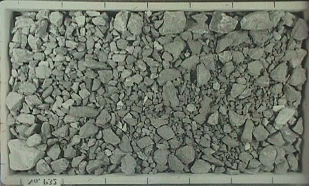
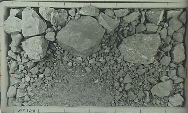
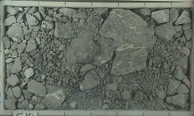
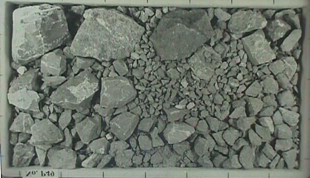
87 Figure 7.2: The 10 photos used in the blind comparison; row-wise P01, P09, P10, P14, P29, P32, P46, P49, P59, P67. Latham et al. (2003) figure A1.