Effects of Ultrasound in Microelectronic Ultrasonic Wire Bonding

Transcription

1 Effects of Ultrasound in Microelectronic Ultrasonic Wire Bonding by Ivan Lum A thesis presented to the University of Waterloo in fulfillment of the thesis requirement for the degree of Doctor of Philosophy in Mechanical Engineering Waterloo, Ontario, Canada, 2007 Ivan Lum, 2007

2 I hereby declare that I am the sole author of this thesis. This is a true copy of the thesis, including any required final revisions, as accepted by my examiners. I understand that my thesis may be made electronically available to the public. ii

3 Abstract Ultrasonic wire bonding is the most utilized technique in forming electrical interconnections in microelectronics. However, there is a lacking in the fundamental understanding of the process. In order for there to be improvements in the process a better understanding of the process is required. The mechanism of the bond formation in ultrasonic wire bonding is not known. Although there have been theories proposed, inconsistencies have been shown to exist in them. One of the main inconsistencies is the contribution of ultrasound to the bonding process. A series of experiments to investigate the mechanism of bond formation are performed on a semi automatic wire bonder at room temperature. 25 µm diameter Au wire is ball bonded and also 25 µm diameter Al wire is wedge-wedge bonded onto polished Cu sheets of thickness 2 mm. It is found that a modified microslip theory can describe the evolution of bonding. With increasing ultrasonic power the bond contact transitions from microslip into gross sliding. The reciprocating tangential relative motion at the bond interface results in wear of surface contaminants which leads to clean metal/metal contact and bonding. The effect of superimposed ultrasound during deformation on the residual hardness of a bonded ball is systematically studied for the first time. An innovative bonding procedure with in-situ ball deformation and hardness measurement is developed using an ESEC WB3100 automatic ball bonder. 50 µm diameter Au wire is bonded at iii

4 various ultrasound levels onto Au metallized PCB substrate at room temperature. It is found that sufficient ultrasound which is applied during the deformation leads to a bonded ball which is softer than a ball with a similar amount of deformation without ultrasound. No hardening of the 100 µm diameter Au ball is observed even with the maximum ultrasonic power capable of the equipment of 900 mw. In summary, the fundamental effect of ultrasound in the wire bonding process is the reciprocating tangential displacement at the bond interface resulting in contaminant dispersal and bonding. A second effect of ultrasound is the softening of the bonded material when compared to a similarly non-ultrasound deformed ball. iv

5 Acknowledgments I would like to thank my supervisors Dr. Y. Zhou and Dr. M. Mayer for their input, support and guidance over the duration of this work. This work was supported with financial assistance from NSERC, Microbonds, MKE Electron Inc., Ontario Centres of Excellence, and OGS. I would like to thank everyone in the CAMJ group at the University of Waterloo for the help and input they provided to this study. I would like to thank Dr. Yuquan Ding for his advice. Finally I would like to thank everyone in the Department of Mechanical Engineering for their support. v

6 To my family. vi

7 Table of Contents Chapter 1 Introduction Objectives Process Description Process Variations Ultrasonic Wedge-Wedge Bonding Ball Bumping Cu wire Ultrasonic Energy Generation of Ultrasound in Wirebonding Effects of Ultrasound in Wirebonding Reciprocating Tangential Displacement at Bond Contact Ultrasonic Effect on Metals Materials Issues in Wirebonding Cu Substrates Cu Wire Insulated Bonding Wires Bonding on Low-k Substrates Equipment and Fixturing Autobonders Manual Bonder Quality Control Pull Test Shear Test Bonding Mechanisms Methods Used to Study Bonding Mechanisms Existing Proposed Bonding Mechanisms Melting vii

8 Deformation Microslip Contact Mechanics and Wear Important Parameters and Their Effects Ultrasonic Power Bonding Force Bonding Time Bonding Temperature Microsensors used to Study Wirebonding Chapter 2 Gold Ball Bonding Mechanism Procedure Results Bonds Made with Low Bonding Force Bonds Made with Higher Bonding Forces Discussion Bond Development Effect of Bonding Force Summary Chapter 3 Aluminum Wedge Bonding Mechanism Procedure Results Bonds Made with Low Bonding Force Bonds Made with High Bonding Forces Discussion Bond Footprint Evolution Effect of Bonding Force viii

9 3.3.3 Effect of Ultrasonic Energy Summary Chapter 4 Effect of Ultrasound on Hardness of Bonded Au Ball Procedure and Experimental Details Procedure Overview Detailed Procedure Experimental Details Feasibility of Using Online Method as Measure of Hardness Results and Discussion Ultrasound Effect on the Hardness of the Bonded Ball Base Comparison 0 mw Ultrasound Medium Ultrasound Level 75 mw Low Ultrasound Level 13 mw High Ultrasound Level 900 mw Effect of Ultrasound Power Level on Residual Hardness Ultrasound Effect on the Deformation of the Ball Deformation Rate of the Ball Bond Summary Chapter 5 Conclusions References Appendix A - Ball Bond Footprints at 80 gf Appendix B - Wedge Bond Footprints at 50 gf. 143 ix

10 List of Tables Table 1.I: Summary of the Main Wire Bonding Techniques/Materials Table 2.I: Number of Bonds Lifted Off Table 2.II: Fretted Annulus Inner and Outer Diameters [µm] Table 2.III: Material Properties used in the Model Table 4.I: Parameters for Forming 100 µm Diameter Au FAB Table 4.II: t-tests Comparing BHHard Obtained With 75 mw Ultrasound and 0 mw Ultrasound with Similar BHDef or Interpolated Equal BHDef. dof in the Table are Degrees of Freedom. t-table is from Reference [64] Table 4.III: t-tests Comparing BHHard Obtained With 13 mw Ultrasound and 0 mw Ultrasound with Similar BHDef or Interpolated Equal BHDef. dof in the Table are Degrees of Freedom. t-table is from Reference [64] Table 4.IIII: t-tests Comparing BHHard Obtained With 900 mw Ultrasound and 0 mw Ultrasound with Similar BHDef or Interpolated Equal BHDef. dof in the Table are Degrees of Freedom. t-table is from Reference [64] Table 4.V: t-tests Comparing BHHard Obtained with Various Ultrasound Powers with Similar BHDef or Interpolated Equal BHDef. dof in the Table are Degrees of Freedom. t-table is from Reference [64] Table 4.VI: Calculated Deformation Rates x

11 List of Figures Figure 1.1: Schematic of bonding equipment setup showing horn with clamped capillary. Lower image showing photograph... 5 Figure 1.2: Illustration of ultrasound propagation along horn and capillary Figure 1.3: Illustration of ball bonding process steps... 7 Figure 1.4: Illustration of wedge-wedge bonding process steps... 9 Figure 1.5: Wedge tool used in ultrasonic wedge-wedge bonding Figure 1.6: Bonded ball bumps on a substrate surface Figure 1.7: Free-air ball formed with Cu wire (a) with 95%N-5%H forming gas, and (b) in ambient air Figure 1.8: Photograph of autobonder Figure 1.9: Photograph of semi-automatic bonder Figure 1.10: Pull test hook Figure 1.11: Force balance during pull test Figure 1.12: Shear tool (shear ram) Figure 1.13: Distribution of normal pressure p and shear traction q over the surface of contact of two elastic spheres subject to a normal force N and a shear force S [47]. 28 Figure 1.14: Illustration of sticking and sliding in a circular contact under constant normal and increasing tangential load, showing transition from microslip to gross sliding Figure 1.15: Development of fretting over the contact circle as the amplitude of oscillating tangential force is increased. (a) lower tangential force, and (b) increased tangential force [47] Figure 1.16: Parameter settings and control profiles during a wire bond Figure 2.1: Capillary geometry used in the study, all dimensions in micrometers Figure 2.2: The two types of bonding outcomes resulting in footprints Figure 2.3: Bond footprints made with 35 gf normal bonding force at various bonding powers. a) Lifted off bond footprint made at 130 mw, and (b) backscatter image of xi

12 same bond showing gold (bright areas). Sheared footprints made at c) 260 mw, and d) 390 mw, noting the directionality of bonding which is in the ultrasonic vibration direction Figure 2.4: Bond footprints made with 80 gf normal bonding force at various bonding powers. Lifted off bond footprints made at a) 130 mw, b) 260 mw, and c) 390 mw paired with each corresponding lifted off ball showing same contact diameter as OD. Sheared footprints made at d) 520 mw, and e) 650 mw Figure 2.4 cont d: Bond footprints made with 80 gf normal bonding force at various bonding powers. Lifted off bond footprints made at a) 130 mw, b) 260 mw, and c) 390 mw paired with each corresponding lifted off ball showing same contact diameter as OD. Sheared footprints made at d) 520 mw, and e) 650 mw Figure 2.5: Bond footprints made with 110 gf normal bonding force at various bonding powers. Lifted off bond footprints made at a) 130 mw, b) 260 mw, c) 390 mw, and d) 520 mw. e) Sheared bond footprint made at 650 mw Figure 2.5 cont d: Bond footprints made with 110 gf normal bonding force at various bonding powers. Lifted off bond footprints made at a) 130 mw, b) 260 mw, c) 390 mw, and d) 520 mw. e) Sheared bond footprint made at 650 mw Figure 2.6: Schematic illustration of the change in footprint morphology from microslip to gross sliding for increasing ultrasonic power. Grey areas indicate fretting while the dashed circle indicates the capillary chamfer diameter. Bonding density is indicated by the cross hatching Figure 2.7: Suggested normal stress distribution at the ball/substrate interface Figure 2.8: von Mises stress distribution for ball bonding at the substrate surface calculated using finite element methods for varying ball/sheet friction coefficients Figure 2.9: Normal stress distribution for ball bonding at the substrate surface calculated using finite element methods for varying ball/sheet friction coefficients Figure 2.10: Mesh used in the numerical analysis. Upper figure shows overall mesh while bottom figure shows mesh at bond interface Figure 2.11: Sensitivity analysis performed on the mesh size of the substrate surface layer under the ball bond xii

13 Figure 2.12: Plot of von Mises stress showing negligible difference with element size smaller than 0.28 µm Figure 2.13: Percent lifted off versus bonding power for normal bonding forces of: a) 35, b) 80, and c) 110 gf. Hollow symbols indicate microslip condition while solid symbols indicate gross sliding. Shaded area indicates gross sliding regime Figure 3.1: Wedge geometry used in the study, all dimensions in micrometers. a) shows side profile view of the tool while b) shows underside of the tool Figure 3.2: SEM top view of wedge-bond showing first bond, second bond, and wire loop Figure 3.3: The two types of bonding outcomes resulting in footprints Figure 3.4: Schematic of the shearing procedure of a wedge-bond (not to scale) Figure 3.5: Percent lifted off versus ultrasonic power for normal bonding forces of: a) 35, b) 50, and c) 65 gf. Hollow square symbols indicate microslip condition while solid square symbols indicate gross sliding. Hollow triangles indicate no bonding. Ten samples per data point Figure 3.6: Bond footprints made with N=35 gf at various ultrasonic powers. a) Lifted off bond footprint made at 65 mw, and sheared bond footprints made at b) 130 mw, c) EDX aluminum map of the same bond (130 mw) showing aluminum as bright areas, d) 195 mw, and e) 260 mw Figure 3.7: Bond footprints made with N=50 gf at various ultrasonic powers. Lifted off bond footprints made at a) 65 mw and b) 130 mw. Sheared bond footprints made at c) 195 mw and d) 260 mw Figure 3.8: Bond footprints made with N=65 gf at various ultrasonic powers. Lifted off bond footprints made at a) no ultrasonic energy and b) 130 mw. Sheared bond footprints made at c) 195 mw and d) 260 mw Figure 3.9: Footprint width for each representative bond versus ultrasonic power for normal bonding forces of: 35, 50, and 65 gf. No value was determined at the parametric combination 35 gf and 0 mw as the footprint contrast was too low to allow measurement xiii

14 Figure 3.10: Schematic illustration of the change in footprint morphology from microslip to gross sliding for increasing ultrasonic power. Shaded areas indicate fretting while bonding density is indicated by the darkness of the shaded area (darker means larger bonding density) Figure 3.11: Suggested normal stress distribution at the wire/substrate interface for a) wedge-bonding and b) ball-bonding Figure 3.12: Postulation of a transition area with bond sticking in the microslip regime, overlaid on the experimental parameter space. Solid square symbols indicate gross sliding condition while hollow symbols indicate microslip Figure 4.1: Schematic of the online procedure for preparing samples and measuring hardness Figure 4.2: Plot showing bonding signals obtained for the online procedure and illustrations showing the corresponding z-position measurements used in the study Figure 4.3: SEM micrographs showing a 50 µm diameter Au FAB made with 25 µm diameter wire after impact with substrate using touchdown detection of 15 mn and contact velocity of 2 mm/sec. Lower photos show the ball bottom and ball top with higher magnifications. Notice the negligible deformations Figure 4.4: Plot showing increasing bonding forces resulting in increasing deformation velocities when operating in the standard mode of the ESEC WB Figure 4.5: Bonding layout for the wire sets used in the experiments. Bond numbers indicate the order that the wires are bonded Figure 4.6: Schematic of the online hardness measure of a wire Figure 4.7: Schematic of the hardness indentation test of a wire cross section Figure 4.8: Plot of online measured height versus microhardness of three different hardness Cu wires. The error bars indicate one standard deviation Figure 4.9: Average calculated ball heights for balls deformed with 0 mw ultrasound power. The error bars indicate one standard deviation Figure 4.10: Average calculated ball deformation for balls deformed with 0 mw ultrasound power xiv

15 Figure 4.11: Average calculated ball heights for balls deformed with 75 mw ultrasound power compared to 0 mw. The error bars indicate one standard deviation Figure 4.12: Average calculated ball deformation for balls deformed with 75 mw ultrasound power Figure 4.13: Average calculated BHHard for balls deformed with 0 and 75 mw ultrasound power. Also shown are the 10 data points of the data sets used for the t- tests and some other deformation load values. The error bars indicate one standard deviation. Not all of the complete set of 10 data points for each average are shown to increase clarity Figure 4.14: Average calculated ball heights for balls deformed with 13 mw ultrasound power compared to 0 mw. The error bars indicate one standard deviation Figure 4.15: Average calculated ball deformation for balls deformed with 13 mw ultrasound power Figure 4.16: Average calculated ball heights for balls deformed with 900 mw ultrasound power compared to 0 mw. The error bars indicate one standard deviation Figure 4.17: Average calculated ball deformation for balls deformed with 900 mw ultrasound power Figure 4.18: Plot showing mean BHHard at different ultrasound levels. Error bars indicate one standard deviation Figure 4.19: Plot showing increasing ultrasound power causing increasing deformation Figure 4.20: The corrected and uncorrected z-positions for the deformation portion of a representative ball from the (0%, 1730 mn) sample Figure 4.21: The corrected z-position profiles for the deformation portion of representative balls from the (a) (0%, 1730 mn) and (b) (30%, 1130 mn) sample xv

16 Chapter 1 Introduction Wire bonding is the most utilized technique for forming electrical interconnections in the microelectronics industry with more than 3 trillion wires annually bonded [1]. Wire bonding is widely accepted because of its flexibility and robustness. In the general wire bonding process a small diameter metal wire (usually 25 µm diameter Au) is bonded with a tool firstly to a metal layer on the microchip (usually Al) and then to a metal layer on the packaging thus forming the interconnection. The most widely used method is thermosonic ball bonding in which ultrasonic energy is combined with thermal energy under a normal bonding force to form the bond. This is a refinement of the process that was first introduced as thermocompression wire bonding in the 1950 s at Bell Labs in which only thermal energy was combined with a normal bonding force [1]. Subsequently, in the 1960s ultrasonic energy was added to the process and called hot work ultrasonic bonding (now called thermosonic) and is credited to Coucoulas [2]. By adding ultrasonic energy lower temperatures could be used which prevented damage to 1

17 the devices and bonding times were shortened. These two benefits resulted in the wide implementation of the thermosonic process in industry. Since that time the process has remained fundamentally the same even though there have been many improvements in wire bonding equipment and throughput rate. The only significant change in technology since the process was developed has been in the ultrasonic frequency used. Before the 1990 s the ultrasonic frequency used was generally about 60 khz. The reason for the selection of the original frequency was not so much through research but the fact that it worked [1]. Current modern autobonders utilize an ultrasonic frequency of about 130 khz which speeds up the process. Although there are competing technologies such as tape automated bonding (TAB) bonding and flip chip, in the foreseeable future wirebonding due to its flexibility and lower cost will remain the leading interconnection production technology. Although the wirebonding technique is widely accepted, at present there is a limited understanding of the ultrasonic bonding process. There is a lack of a quantitative understanding of the bonding mechanism [1]. The three existing theories on the bonding mechanisms do not adequately describe it and are not well accepted [3]. For example one area of great debate is the role of ultrasonic energy in bonding. In order to make advancements in wire bonding, a thorough understanding of the process mechanisms must be achieved. Once this is accomplished new materials combinations and/or increased productivity may be realized in ultrasonic bonding. It is widely accepted that wire bonding is a solid state process [4]. Various investigations to support this includes studies of bonding at liquid nitrogen temperatures [5] and examination of the bond interface in a transmission electron microscope (TEM) 2

18 [6]. One of the requirements to form metallurgical bonding is a relatively contaminant free surface [7]. Without melting occurring some other method of contaminant dispersal is required. For example, in cold pressure welding it is the applied pressure and subsequent deformation that breaks up the oxide layer [8]. It is suggested by Mayer [9, 10] that relative motion at the ball/pad interface, leading to gross sliding and oxide removal is important in bond formation. Because of this relative motion, wear may occur leading to the dispersal of contaminants. With the increasing demands of integrated circuits (ICs) with ever increasing clock speeds methods need to be found to accommodate this trend since the current materials used have physical limitations. One alternative is to replace the standard aluminum metallization with copper. Copper has a lower electrical resistance than aluminum [11]. However, copper forms an oxide layer at the elevated temperatures of thermosonic bonding which hinders bonding [12-18]. Therefore, copper substrate is used in some parts of this study. This allows both a development of a bonding process for copper and also facilitates an understanding of the bonding mechanisms. 1.1 Objectives This work is performed with the intention of gaining a better understanding of the fundamentals of the wirebonding process. The mechanism of bonding evolution is to be determined. The processes of ultrasonic ball bonding and ultrasonic wedge-wedge 3

19 bonding are to be compared. The effect of ultrasound on the hardness of the bonded ball is to be determined. In this introductory Chapter, Section 1.2 will describe the thermosonic wirebonding process. The different variations of the wirebonding process will be discussed in Section 1.3. In Section 1.4 the fundamentals of ultrasonic energy are discussed. Section 1.5 discusses the current materials issues in wirebonding. Wirebonding equipment are described in Section 1.6 with wirebonding quality control following in Section 1.7. The methods used to study the bonding mechanism and the existing proposed bonding mechanisms are discussed in Section 1.8. Finally, the Chapter is finished with a discussion of the effect of bonding parameters in Section Process Description The predominantly used thermosonic ball bonding process will be described. Both ultrasound and thermal energy are used to form the bond. A tool (capillary) is used to provide the normal bonding load to the wire. The capillary is clamped into the horn as shown in Figure 1.1. The ultrasonic transducer which is made from a piezoelectric material (discussed more in ultrasonic energy section) is attached to the base of the horn and the ultrasound is propagated as a longitudinal wave along the length of the horn which is then propagated as a transverse wave in the capillary as shown in Figure 1.2. Vibration nodes may appear in the tool (the number and location of nodes depends on both frequency and tool geometry) with a resultant oscillating tangential displacement at 4

20 the tip of the tool. The thermal energy is usually provided by a heated clamping stage which holds the material to be bonded. Figure 1.1: Schematic of bonding equipment setup showing horn with clamped capillary. Lower image showing photograph. 5

21 Figure 1.2: Illustration of ultrasound propagation along horn and capillary. The bonding process can be described with the aid of Figure 1.3 and is as follows: 1. First, a free air ball (FAB) is formed on the end of the wire by an electric arc. The molten Au forms a ball due to surface tension. The first bond site (bond pad) is located and the capillary is brought down, pulling the ball into the chamfer. 2. When the capillary makes contact with the pad the ball is pressed onto it. A normal bonding force is applied and after a set amount of time ultrasonic energy is switched on for a set amount of time (about 20 ms) forming the bond. 3. The capillary is then raised, with the ball bond (first bond) remaining on the bond pad. 4. The capillary moves to the second bond site (lead) forming a wire loop. 5. The capillary is brought down. Once again, after the normal force is applied, ultrasonic energy is switched on to form the crescent bond (second bond). 6. The capillary rises. 7. At a preset height clamps close on the wire to break the wire at the crescent bond with the broken wire end called the tail protruding from the end of the capillary to be flamed off again with the electric arc and the cycle repeated. In this fashion a wire interconnect has been formed and a FAB has been prepared to be used for the next bond connection. 6

22 Figure 1.3: Illustration of ball bonding process steps. 1.3 Process Variations There are significant variations on the wire bonding technique depending on the specific application and different wire materials and metallization materials combinations can be substituted as well and are summarized in Table 1.I and are described in 7

23 subsections to Commonly used wire materials are Au, Al, and Cu which all have in common high ductility. The material combinations that can be bonded are usually ductile metals, i.e. Au wire on Al metallization, Cu wire on Ag metallization. Table 1.I: Summary of the Main Wire Bonding Techniques/Materials. Procedure Thermosonic Ball Ultrasonic Wedge Cu Ball Bonding Standard Wire Material Main Applications Shielding Gas Au Microelectronics None Al Power devices, None Automotive Cu Microelectronics 95%N 5%H Ultrasonic Wedge-Wedge Bonding Ultrasonic wedge-wedge bonding is the second most predominant wirebonding technique and the first ultrasonic wirebonding technique developed [1]. In the wedgewedge bonding process there is no ball formed on the end of the wire, which is usually aluminum, and the wire itself is pressed with a tool against the bond location. Normally, wedge bonding is performed at ambient temperatures. Figure 1.4 shows the ultrasonic wedge bonding process and is similar to the thermosonic ball bonding process except for the absence of ball formation and thermal energy. The tool in this case is called a wedge and is shown in Figure 1.5. The bonding process can be described with the aid of Figure 1.4 and is as follows: 8

24 Figure 1.4: Illustration of wedge-wedge bonding process steps. 1. First, the wedge with the protruding length of wire called the tail descends to the first bond position. 2. When the wedge makes contact with the pad the wire is pressed onto it. A normal bonding force is applied and after a set amount of time ultrasonic energy is switched on for a set amount of time (about 20 ms) forming the bond. 3. The wedge is then raised, with the bond remaining on the bond pad. 4. The wedge moves to the second bond site forming a loop. 5. The wedge is brought down. Once again, after the normal force is applied, ultrasonic energy is switched on to form the second bond. 9

25 6. The wedge rises. 7. At a preset height clamps close on the wire to break the wire at the second bond. 8. The clamps feed the wire forward to form the tail protruding from the end of the wedge and the cycle may then be repeated. In this fashion a wire interconnect has been formed. Larger diameter wires of up to 500 µm that are used to connect high power devices may be produced using the ultrasonic wedge bonding technique [1]. Figure 1.5: Wedge tool used in ultrasonic wedge-wedge bonding Ball Bumping In this technique only the ball is bonded to the substrate and is called a ball bump. One application of ball bumping is to form studs for flip chip interconnects. The process follows the first 3 steps of the thermosonic process but after the ball is bonded onto the substrate the clamps close and the wire is broken leaving a bonded ball on the substrate. The process then repeats. Figure 1.6 shows bonded ball bumps on a substrate surface. 10

26 Figure 1.6: Bonded ball bumps on a substrate surface Cu wire A recurring trend has been to substitute Cu wire for the Au wire in thermosonic ball bonding [19, 20, 21]. There are two main reasons for the interest in Cu wire. The first is that Cu has a lower electrical resistance than Au [22, 23]. The second is that Cu wire is less expensive than Au [24]. Cu can also be replaced for the wedge bonding process. However, there are challenges when using Cu wire. Due to the increased hardness of the Cu wire there may be bondability issues [25, 26, 27]. Also when using Cu wire for ball bonding a shielding gas needs to be used for ball formation. Typically a forming gas of 95% Nitrogen 5% Hydrogen is used [28]. In ambient atmosphere the ball formation will result in oxidized and misshaped balls as shown in Figure

27 Figure 1.7: Free-air ball formed with Cu wire (a) with 95%N-5%H forming gas, and (b) in ambient air. 1.4 Ultrasonic Energy Ultrasound is defined as sound with a frequency above 12 khz and is thus inaudible to the human ear. Ultrasound has found many applications in industry such as the familiar ultrasound used in medical imaging, and ultrasonic cleaning just to name two. In ultrasonic wirebonding the ultrasonic energy is an important factor in the process Generation of Ultrasound in Wirebonding The design of an ultrasonic system for wirebonding consists of an electronic power supply, control system, ultrasonic transducer, and horn. As shown in Figure 1.2 the ultrasound is produced by an ultrasonic transducer and is then conducted along the 12

28 horn. The horn transmits the ultrasonic energy from the transducer to the capillary and is designed to amplify the vibration amplitude to larger values at the capillary end. The transducer is made of piezoelectric material which has the property that it will create a force when voltage is applied to it. With a voltage applied at the input frequency the output is a displacement from the transducer at that same frequency. Typical wirebonders use ultrasound frequencies of 60 khz or more recently 130 khz. The oscillating displacement output from the transducer is propagated along the horn as a longitudinal wave and as a transverse wave in the bonding tool as shown in Figure 1.2. Vibration nodes may exist in the bonding tool depending on the applied frequency and tool geometry. There will be a resultant oscillating tangential displacement at the tool tip Effects of Ultrasound in Wirebonding Reciprocating Tangential Displacement at Bond Contact The main effect of the application of ultrasound is the resulting oscillating displacement at the tool tip. This displacement at the tool tip is fundamental and required in the ultrasonic wire bonding process. The oscillating displacement at the tool tip and thus at the wire/substrate interface aids in the cleaning of the surfaces allowing subsequent intimate metal/metal contact and bonding. 13

29 Ultrasonic Effect on Metals There are two effects of ultrasound on metals: ultrasonic softening and ultrasonic hardening. In ultrasonic softening the static stress necessary for plastic deformation of metals is decreased only during the application of ultrasound. On the other hand, ultrasonic hardening as the name implies leads to a hardening and is observed as a residual effect after the ultrasonic irradiation is stopped. Langenecker [29] studied the effects of ultrasound on the deformation characteristics of metals. Intense ultrasound and applied heat have similar effect on the reduction of the stress required for deformation. This effect of ultrasound is referred to as ultrasonic softening. The ultrasound softening effect can be achieved at much lower applied energy levels as compared to thermal energy. This higher efficiency of lowering yield stress has been suggested to be due to the attenuation of ultrasonic energy only at the points that affect deformation such as dislocations and vacancies [30] whereas thermal energy is uniformly distributed across the bulk material. It was shown that throughout the frequency range of 20 khz up to 1000 khz this softening would occur. Ultrasonic softening only occurs when ultrasound is switched on. The material shows no residual effects once ultrasound is removed. With higher applied ultrasonic powers the apparent yield stress decreases more. However, at very high power levels a residual hardening effect occurs [29]. The material has thus been permanently hardened. 14

30 1.5 Materials Issues in Wirebonding Cu Substrates Aluminum is typically used as bond pads for thermosonic ball bonding of gold wire. With the increasing demands of IC s with ever increasing clock speeds methods need to be found to accommodate this trend since the current materials used have physical limitations. One alternative is to replace the aluminum metallization with copper. It was shown that it was possible to produce reliable thermosonic gold ball bonds on copper substrate by utilizing a shielding gas atmosphere [31] Cu Wire Cu is harder than Au and leads to challenges in bonding with defects such as chip cratering occurring [25, 26]. Another challenge is the repeatability of the tail bond which is formed during the wedge bond formation [27]. It was suggested that the different microstructural and material properties of Cu compared to Au leads to the variability in the breaking of the wire after the wedge bond [27]. The tail bond controls the length of tail available for the FAB formation. Weak tail bonds will lead to the wire lifting off of the substrate before the tail bond breaking stage and the tail will recede into the capillary resulting in stoppage of the process due to the absence of the tail. 15

31 1.5.3 Insulated Bonding Wires As miniaturization combined with increased number of signal connections on a microchip continues unabated into the future insulated bonding wires offer a viable solution to meet the challenges. The main feature of insulated bonding wires is the insulation on the wire which prevents wires from short circuiting. Insulated bonding wires offer increased wire densities and new bonding wire layouts for the packaging solutions of the future [32] Bonding on Low-k Substrates Low-k materials can lack the mechanical stability to survive the wirebonding process. Low-k materials are becoming more common as insulation layers under the metallization layers [33, 34, 35] in microchips. The variable k is used for the dielectric constant of an insulating material. A lower k value means better insulation properties with air being the best insulator with a k value equal to one. As the trend of signal speeds carried by the interconnection wires increases a better insulating material (lower k value) is required to eliminate the cross talk between wires. The standard insulation is SiO 2 with a k equal to 4.1 [35]. New lower k materials being used with k values less than 3 (typically about 2.7) [35] possess much lower thermo-mechanical stability than SiO 2. In order to use the wirebonding process on low-k materials, damage to the low-k material is prevented either through adjustment of the bonding process or the structure of the low-k material, or - most promising - adjusting both. 16

32 1.6 Equipment and Fixturing Autobonders Autobonders are fully automated bonders that when provided with a bonding program will perform continuous bonding without operator intervention except for when problems arise. These are the bonders used for most production. Figure 1.8 shows an advanced auto ball bonder. All of the functions of the bonder are controlled by software. Bond programs will include all parameters required to perform the bonding including bond positions and parameters and material handling parameters. Each bond has its own specific parameters. If changes are required it is only a matter of changing the parameters in the program. Advanced vision systems comprising of a camera mounted to the bond head and software are used for programming and bonding. Computer monitors display both the computer interface and vision system information. There is also a microscope for viewing the bonds. Autobonders have automated material handling systems which move material from the input stage through the bonding area and into the output (storage) stage. During the bonding the material can be held in place by vacuum and or an upper clamping plate. For production, material is usually provided in strips with many dies on a strip, although single pieces may also be bonded. In auto ball bonders it is the bondhead that moves to perform bonding with the material to be bonded remaining stationary. However, in auto wedge bonders, in addition 17

33 to the bondhead moving, the material may also be rotated since the first and second bonds are required to be parallel. Figure 1.8: Photograph of autobonder Manual Bonder Manual bonders, Figure 1.9, are used for research and development and small quantity bonding. A fixture called the bonding stage is used to clamp the material and 18

34 perform bonding on. Clamping can either be by vacuum or spring loaded clamping tabs and is performed manually. The bonding stage is placed on the x-y table which is controlled by the operator via a mechanical micromanipulator. By observing through the microscope and by moving the x-y table via the micromanipulator the operator locates the desired bond position and triggers an automatic bonding procedure by pressing a button. Each bond is automatically made by pressing the button. In contrast to the auto bonders the bonding tool remains fixed in x, y space. The parameters for the bonding are selected by buttons/dials on the machine and may be displayed on an LCD display. The parameters selectable with a manual bonder are much less than what are available with an autobonder and are limited to ultrasonic power, bonding time, bonding force, search height, and loop height. Figure 1.9: Photograph of semi-automatic bonder. 19

35 1.7 Quality Control There are two main standardized tests for the wirebonding process. Each test is typical for testing one type of wirebond; the ball type (first bond) or the wedge type (second bond) Pull Test A hook as used on a pull tester is shown in Figure It is used for testing the strength of either the first or the second bond for both ball bonding and wedge-wedge bonding. In this test a hook is placed under the wire loop, pulled upwards with a controlled speed, and the force required to break the bond is recorded. The pull test is standardized in [36] and [37]. According to the latter, the required minimum pull force is 3 gf (1 gf = 9.8 mn) for a process with a 25 µm diameter wire. The pull force value is variable depending on where the hook is placed as shown by the force vectors in Figure The hook is placed closer to the bond to be tested. For a sufficiently strong wedge bond the wire breaks in the heel region of the bond. When testing a moderately strong Au ball bond, the wire breaks in the neck region of the ball. Therefore, the strength of some ball bonds cannot be fully characterized with the pull test. However, a lower quality limit can be assured and the pull test remains in use for assuring the first and second bond quality of many production processes. 20

36 Figure 1.10: Pull test hook. Figure 1.11: Force balance during pull test Shear Test A close-up of a shear tester is shown in Figure In this test a shear ram (shear tool, shear chisel) is used to shear through the bond or the wire at a fixed height 21

37 from the surface of the bond pad (typically about 3 µm). The shear test is standardized in [38]. It measures the maximum force required to shear the bond. A sufficiently bonded ball is sheared through the ball material leaving a layer of the ball material bonded onto the substrate. A poorly bonded ball leaves little material behind when sheared. It effectively delaminates from the interface. The industry minimum strength required depends on the material combination used, the diameter of the bond connection, and the standard deviation of the shear force results. The shear strength is calculated as the shear force divided by the nominal bond area. Alternatively this test can be used to shear through a wedge bond to test the shear strength of the wedge bond itself. However, this is not a standardized test. Figure 1.12: Shear tool (shear ram). 22

38 1.8 Bonding Mechanisms Methods Used to Study Bonding Mechanisms The most widely used technique in the study of bonding mechanisms is the study of the bond footprint [1]. The footprints are the impressions left on the substrate surface and show the surface morphology changes and microwelds that occur from the bonding operation. The footprints may be obtained either by mechanically removing the wire (i.e. peeling the wire off) or chemically etching the wire away. A common method used to determine the amount of bonding of a gold ball on Al metallization is to etch the balls off of the substrate and observe the underside of the balls. The discoloration in the ball underside will indicate intermetallic formation and bonding [1] Existing Proposed Bonding Mechanisms It is widely accepted that the wirebonding process is a solid state process. In order to create a bond between two metals the surfaces must be relatively contaminant free [7] and the bonding surfaces have to be brought into intimate contact. Without melting occurring some other method of contaminant dispersal is required. There have been three main theories proposed in literature to account for the bonding mechanism in ultrasonic wirebonding and include melting, deformation, and microslip theory. 23

39 Melting One of the very first bonding mechanism theories proposed was that of melting. It is postulated that the interfacial movement caused by ultrasonic energy caused rubbing, heating and then even melting of the interfaces resulting in bonding [39]. There has since been many inconsistencies shown in this theory from the large quantity of experimental evidence showing that although there is a temperature rise, that bond temperatures do not approach the melting point of the materials. For example bonding performed at liquid nitrogen temperatures show that no bubbles are observed, indicating that temperature rise is very low [40, 41]. Therefore, it is concluded that the observed temperature rise does not create the bonding but is rather a by-product of the bonding process. Also a TEM study which measured diffusion distances of vacancies to the grain boundaries indicates that bond temperatures are no more than about 250 C [6]. Furthermore, examination of the bond interface in the same TEM study indicates no evidence of melting. Melting may be present in wirebonds made under non-optimal conditions of too high ultrasonic power producing overdeformed bonds. In this case the friction energy is large and temperature rise may be substantial. In particular if bonding on Sn - a material melting at a relatively low temperature - melting may be evident when studying the bond interface [42]. However, at optimal bonding parameters there is no melting observed. Even when bonding on Sn which has a low melting point, under normal conditions there is no melting. Therefore, the evidence suggests that melting is not required for successful ultrasonic wire bonding. 24

40 Deformation Another mechanism brought forth to explain the bond formation in ultrasonic bonding is the deformation mechanism. In this theory it is postulated that the interfacial extension due to the lateral deformation of the wire results in displacement of contaminants and reveals fresh metal underneath which will readily bond. This appears to be valid for thermocompression (no ultrasonic energy) bonding. Takahashi et al. [43] performed a numerical analysis of the interfacial contact process in thermocompression wire bonding using a simplified model. It is concluded that a wire height reduction of 0.5 is required to produce a strong peripheral bond, and the result is comparable to the deformation required for cold pressure welding. Harman and Leedy [40] noted the similarity of the deformation in thermocompression and thermosonic bonding and suggest that the only difference in the two processes is the form of energy used to cause plastic flow. However, this is shown to be an overly simplified view of the effects of ultrasonic energy as studies have shown that bonds made with the same amount of deformation with and without ultrasonic energy demonstrated different bond strengths and amount of bonding in Au ball bonding [44]. This shows that deformation theory alone cannot be used to explain the thermosonic bonding process adequately Microslip Chen [45] proposed a microslip based theory of the ultrasonic bonding mechanism in 1972, which is based on the work performed by Mindlin [46] on 25

41 compliance of elastic bodies. Microslip theory will be discussed in detail in the next section. Chen stated that the ultrasonic energy results in a tangential force being applied in a reciprocating manner. He then suggested that at low vibration amplitudes microslip will initiate at the periphery of the bond according to microslip theory. It was further suggested that the microslip would displace contaminants from the surfaces revealing clean metal. Bonding is the result of adhesion built upon asperity bridges which are created when the clean metal bodies come into contact under the combination of normal and tangential forces. Once the bonding exists then diffusion of the contacting metals may occur with the elevated temperatures of bonding. This theory was not widely accepted as there was no experimental evidence to confirm this. However, it is useful to study in greater detail the contact mechanics of the interface as it will be later shown that the classical contact mechanics model which is based on elastically deformed spheres contacting spheres or plates can be used to describe aspects of the wirebonding process which has a similar geometry Contact Mechanics and Wear In thermosonic wire bonding the bonding force and ultrasonic vibration are applied to the ball/pad combination by the bonding tool. The ball/pad situation can be simplified as a contact pair under both normal and tangential forces, which has been extensively studied. When two surfaces in contact, are subjected to both normal force (N) and tangential force (S), gross sliding on a macroscopic scale initiates when the tangential force exceeds a critical value, µ s N, where µ s is the coefficient of static friction. If the 26

42 tangential force is less than the critical value, no apparent displacement occurs. However, the tangential force will set up strains so that a minute tangential displacement of one body relative to the other must occur [47]. Mindlin [46] has studied the compliance of two perfectly elastic spheres subjected to both normal force N and tangential force S. When the spheres are brought into contact under normal force N the contact area is over a circle of radius a, and is proportional to N 1/3. The normal pressure distribution over the contact circle is [46]: p = 3N 2πa 2 1 x a 2 2 y a 2 2 1/ 2 Equation 1.1 With the addition of tangential force S, a shear traction q is introduced over the contact area which results in the required tangential displacement of one body relative to the other [47]. Figure 1.13 shows the shear traction q distribution without slip. It can be seen that the traction would rise to infinity at the periphery. Obviously an infinite traction force is not attainable. Therefore the material will slip to relieve the stress. This slip at the periphery is on the order of µm [48] and is termed microslip. The microslip occurs over an annulus a <r<a, while there is no slip occurring over the circle of radius a. The no slip region is known as the stick region. Figure 1.14 shows a schematic of the stick and microslip regions in a circular contact undergoing microslip. Mindlin [46] provided an equation to calculate the size of the microslip annulus: S a' = a 1 µ s N 1 3 Equation

43 where N is the normal force, S is the tangential force, µ s is the coefficient of static friction, a is the annulus inner radius, and a is the contact radius [46]. Figure 1.13: Distribution of normal pressure p and shear traction q over the surface of contact of two elastic spheres subject to a normal force N and a shear force S [47]. The slip annulus grows inwards with increasing tangential force up to the point of gross sliding at which point the microslip annulus has grown to the center of the contact circle as shown in Figure The shear traction q distribution with microslip is shown in Figure

44 Figure 1.14: Illustration of sticking and sliding in a circular contact under constant normal and increasing tangential load, showing transition from microslip to gross sliding. It is believed that with relative motion of contacting surfaces there will be wear occurring [49]. This wear under microslip conditions causes fretting wear, which is common in industry for clamped connections experiencing oscillating tangential forces [50, 51]. The wear of material will occur according to [52]: H 1 t = d Equation 1.3 K PV 29

45 where t is the duration of wear, d is the depth of material worn, P is the mean (nominal) pressure, H is the hardness of the material, K is the wear coefficient constant, and V is the sliding velocity. With the removal of surface material, fresh underlying material will be exposed which may promote bonding. A study by Johnson [47] on the effect of oscillating tangential forces on the surface of materials lends support to Mindlin s theories. Johnson studied elastic spheres pressed against elastic plates which is similar to the geometry encountered in ball bonding. Johnson showed that before the onset of gross sliding, a fretted annulus due to microslip was observed on the surface of the plate. Figure 1.15 shows some of the results. As the magnitude of the tangential force is increased the inner radius of the annulus grows inwards up to the point of sliding. These results confirmed Mindlin s equations. (a) (b) Figure 1.15: Development of fretting over the contact circle as the amplitude of oscillating tangential force is increased. (a) lower tangential force, and (b) increased tangential force [47]. 30

46 1.9 Important Parameters and Their Effects There are many parameters in the wire bonding process. However, the most important parameters of ultrasonic power, bonding force, bonding time, and bonding temperature will be described in this section Ultrasonic Power Ultrasonic power is controlled by the amplitude of the piezoelectric transducer. The resulting vibration amplitude of the bonding tool can be measured directly with a laser interferometer, fiber optic probe, or capacitor microphone [53]. With direct measurement methods it was found that the vibration amplitudes of both unloaded and loaded tools were proportional to the power setting of the ultrasonic generator [53]. Ultrasonic power is shown to be the most important parameter in bond formation [54] and increasing it increases bond strength [41]. The increased bond strength with increased ultrasonic power is due to the increased displacement at the interface and subsequent increased cleaning of the surfaces. With cleaner surfaces more intimate contact between clean metal surfaces will occur and the result is more bonding. Ultrasonic energy also contributes another effect in the bonding process and that is the apparent lowering of the yield stress of metals [29]. A higher ultrasonic power will result in more deformation of the ball bond with other parameters being held constant. 31

47 1.9.2 Bonding Force There are two main bonding forces in a modern bonder. They are impact force and bonding force as shown in the bonding force profile plot in Figure Standard industry practice is to select the impact force to be about two times the value of the bonding force. Generally the impact forces selected in production practice results in most of the ball deformation occurring in the impact stage and during the subsequent ultrasound application little additional deformation of the ball occurs [55]. Figure 1.16: Parameter settings and control profiles during a wire bond. The normal bonding force acts to keep the ball in contact with the bond substrate. The normal bonding force must also be at a sufficient level to couple the ultrasonic 32

48 energy to the materials to be joined. It has been suggested that high forces decrease bonding by limiting interfacial sliding of the ball [9]. The vibration amplitude at the tool tip decreases in an exponential manner as the bonding force increases under constant ultrasonic power [53]. With higher bonding force the displacement of the bonding tool will be less and the ultrasound power needs to be increased to have similar bonding [56] Bonding Time It has been shown by researchers that most of the bonding occurs in approximately the first 12 ms of bonding time, dependent upon the parameters [10]. Shorter bonding times are preferred for increased productivity in industrial applications. For bonding on difficult materials a longer time may be useful as it allows more time for ultrasonic reciprocating displacement to occur and thus more cleaning of the surfaces Bonding Temperature When bonding on Ag plated Cu lead frames, bonding temperatures are 220ºC to 240ºC. When bonding on polymer based substrates, bonding temperatures used are usually about 120ºC to 150ºC. Temperatures that are too high may damage the components being bonded. The additional energy provided by the elevated temperatures assists in the bond formation and increases the bonding throughput. Another effect of the increased temperatures that may aid in bonding is the elimination of surface contaminants 33

49 as was shown by Jellison [57]. However, elevated bonding temperatures may introduce an oxide layer on many materials such as copper which will hinder bonding [18] Microsensors used to Study Wirebonding There have been many attempts to monitor the temperature during bonding and have mainly used thermocouples. The most extensive study of the use of sensors for monitoring of bonding was undertaken by Mayer [9, 10, 58, 59]. Mayer used in-situ microsensors to measure process data such as bonding force, bonding temperature, and bonding shear stress. The bonding forces are measured with pieozoresistive complementary metal oxide semiconductor (CMOS) microsensors located under the bond pad. The temperature is measured by lines of aluminum placed around the bond pad and is based on the change in resistance of the aluminum lines with changes in temperature. After the resistance-temperature relationship is calibrated to known temperatures the absolute temperature can be derived. Of particular interest is the conclusion arrived upon from the shear stress measurements [9]. It is concluded that there existed stick-slip motion at the bond interface based on analysis of the harmonics in the frequency response. The frequency analysis shows 4 phases in bond formation. In Phase 1 the ball and surface slide at the same velocity, here the ball is sticking to the surface. The second phase starts after about 0.5 ms. Phase 2 is characterized by the increase in the third harmonic, which indicates sliding on the ball-substrate interface, and shows bonding. It is suggested that the interfacial slip leads to oxide removal and subsequent bonding. At low ultrasonic power 34

50 the third harmonic does not exist and so Phase 2 does not occur and there is no bonding. In Phase 3 metallurgical bonding is forming. In Phase 4 the harmonics undergo little change. The microsensor used by Mayer et al. [59] to measure temperature yields an average temperature close to the bonding interface. It measures an average temperature due to the placement of the aluminum sensing lines around the outside of the bond pad. In bonding experiments the temperature change measured by such a microsensor typically is not more than 1 K with a response time shorter than 1 ms [60]. There is a drawback in using the above mentioned temperature microsensor and that is that it measures the temperature near the bonding interface. In order to extrapolate the temperature of interest, i.e. under the ball bond, a finite element model would have to be incorporated using the experimentally measured temperature. Mayer and Zwart [60] developed a finite element model to estimate the average temperature of the bond interface if the microsensor temperature is known and it is concluded that no more than a 10 K average temperature increase is expected at the contact zone. Recently in 2005, there has been developed a temperature microsensor that is CMOS compatible and is embedded under the bond pad [61]. Due to the location of the microsensor, a direct measurement of the temperature at a position under the ball bond during bonding can be obtained. The microsensor is an aluminum polysilicon thermopile sensor and has higher sensitivity and signal-to-noise ratio compared to the resistive microsensor described previously. The thermopile is a group of thermocouples configured in such a manner that they are connected electrically in series and thermally in 35

51 parallel. By using this type of microsensor a more representative measure of the bond interface can be obtained. Utilizing temperature microsensors are shown to be a feasible technique to optimize bonding forces [59]. It is shown that the normalized rate of the resistance increase until peak bonding is achieved correlates to the shear strength of the bonded ball (under varied bonding forces) with higher rates of resistance increase corresponding to higher shear strength. At low or excessive bonding forces the normalized rate of resistance increase is low indicating low frictional energy. At optimized bonding forces the rate of the resistance increase is maximum showing maximum frictional energy. This technique of utilizing temperature microsensors for optimization of bond shear force would be much faster than the traditional method of shear testing bonded balls to obtain bond shear forces and may be completely automated. Mayer and Schwizer [58] with the aid of microsensor force measurements developed an analytical model based on ultrasonic friction power at the bond interface to describe the development of bonding in thermosonic ball bonding. The model incorporates material properties, coefficient of friction, and bonding parameters of: bonding load, time, and ultrasonic power. In order to use the model it is required to experimentally perform bonding to obtain a value for the coefficient of bond growth used in the developed model. The coefficient of bond growth is different for each bonding system and thus needs to be experimentally determined for each new bonding system. The main benefit of the model is that it can aid in understanding how process parameters affect the bond strength/development. The model can be a useful tool in industry as it can be used to obtain process windows. For example in a known materials system if the 36

52 geometry of ball bond is changed the model can be used to quickly determine new optimal bonding parameters without having to perform a complete design of experiments study to obtain the new bonding parameters. 37

53 Chapter 2 Gold Ball Bonding Mechanism This chapter discusses an experimental study performed to understand the bonding mechanism occurring in ultrasonic gold ball bonding. It is shown that a modified microslip model can explain the development of bonding with relative interfacial tangential displacement and the resulting cleaning effect important in bond formation. Finally, a model is developed to explain a mechanism observed during the development of bonding. 2.1 Procedure 25 µm gold wire (AW8) manufactured by American Fine Wire is used to ball bump on 1 mm thick OFHC copper substrates supplied by Good Fellow Corporation. 38

54 The substrates are metallographically polished with Al 2 O 3 up to a surface finish of 0.05 µm prior to bonding so that the surface roughness would be similar to those on thin film bond pads. The capillary used was a Small Precision Tools part #SBNE-35ED- AZM-1/16-XL with the geometry as shown in Figure 2.1. Figure 2.1: Capillary geometry used in the study, all dimensions in micrometers. Gold ball bumping is performed on a Kulicke & Soffa 4524D manual ball bonder (operating at 60 khz ultrasonic frequency), Figure 1.9, with the copper substrate at ambient temperature. Various parametric conditions were selected and 10 bonds were made at each combination of parameters. The normal bonding forces used were low, medium, and high forces of 35, 80, and 110 gf (1 gf = 9.81 mn) respectively with the 39

55 bonding time held constant at 1000 ms. In the following discussion one representative bond has been selected from each group of 10 bonds made at the same set of parametric conditions. In order to facilitate more detailed understanding of bonding mechanisms, bond footprints were examined. Two types of bonding outcomes were obtained: lifted off and sticking, resulting in lifted off, and sheared footprints respectively as shown in Figure 2.2. If the bond was weak it would result in a lifted off footprint on the substrate surface. This would occur in the final step of the bond cycle (wire break) if the wire did not break but instead lifted the ball off at the bond interface because the bond was weaker than the wire. On the other hand, if the bond was stronger than the wire, the ball would remain on the substrate (sticking) when the wire was torn, and would subsequently be sheared with a DAGE 4000 (Dage Industries Inc. California) shear tester at a tool height of 3 µm to obtain the sheared footprint. The bond quality could be categorized by a simple sorting model, with lifted off ball bumps as poor quality, and bumps remaining on the substrate (sticking) as better quality. The morphological features of the bond footprints were examined using an SEM. The presence of fractured localized welds (microwelds) in the footprint indicated metallurgical bonding and could be identified by the presence of gold left from the wire. The distribution of the bonded and/or fretted areas aided in the understanding of the bonding mechanisms. 40

56 Figure 2.2: The two types of bonding outcomes resulting in footprints. 2.2 Results Bonds Made with Low Bonding Force An earlier bond development study found that at normal bonding force and bonding time settings of 35 gf and 1000 ms respectively, optimum bonds (based on bond shear force) were made. Therefore, the effect of varying power at these settings was examined. In these results it should be remembered that the capillary chamfer diameter is 51 µm and is clearly indicated in the following figures. 41

57 At 0 mw bond power no fretting was observed and all 10 bonds lifted off as tabulated in Table 2.I. When bonding power was increased to 130 mw all 10 bonds lifted off during bonding, however peripheral fretting at the contact diameter was seen in all bonds of this group and a typical footprint is shown in Figure 2.3(a) as a secondary electron image. Figure 2.3(b) is the backscatter electron image of the same footprint shown in Figure 2.3(a). In backscatter electron imaging gold shows up as bright areas compared to the copper which appears darker since gold has higher atomic density than copper. It can be seen that there was bonding in the peripheral area indicated by the transfer of gold onto the substrate. Table 2.I: Number of Bonds Lifted Off. Bonding Power [mw] Normal Bonding Force [gf] However, not all of the bright areas in the secondary electron image (Figure 2.3(a)) were identified as gold in the backscatter electron image (Figure 2.3(b)) and indicates that there were areas on the substrate contacted by the ball which underwent a change in surface morphology but did not have adherent gold upon observation after bonding. In the areas where it appeared bright in the secondary electron image (Figure 2.3(a)) but not correspondingly so in the backscatter electron image (Figure 2.3(b)) there may have initially existed gold bonding but when the ball lifted off, the gold would have 42

58 remained completely on the gold ball and not the substrate. There is also the possibility that no gold bonding ever occurred in those areas because of insufficient contaminant removal. Despite the limitations of the foregoing discussion it can still be concluded that the bright areas in secondary imaging may indicate the occurrence of fretting and that these fretted areas may or may not result in bonded areas as indicated by the presence of gold. It appears from Figure 2.3(a) that there existed a fretted annulus inner diameter (ID) of about 45 µm with the fretted annulus outer diameter (OD) about 49 µm (Table 2.II). With an increase of bonding power to 260 mw stronger bonding was seen as none of the bonds lifted off during bonding (Table 2.I). Figure 2.3(c) shows a sheared fracture surface of a ball bump made at 260 mw that remained on the substrate surface. Bonded areas may be seen across the entire footprint surface including the center area whereas this was not observed for the lower power bonds (Figure 2.3(a)). It was also observed that there was localized bonding at the chamfer diameter. Some of the bonded areas in Figure 2.3(c) appeared to be elongated in the ultrasonic vibration direction. The OD increased to about 56 µm (Table 2.II) but the ID was now difficult to demarcate due to the large bonding across the entire footprint surface. At the highest bonding power used of 390 mw, none of the bonds lifted off during bonding. A sheared bond footprint made at 390 mw is shown in Figure 2.3(d) and it was measured that the OD increased to about 61 µm. There also appeared to be more bonded area compared to the bonds made at the lower power (Figure 2.3(c)). 43

59 Figure 2.3: Bond footprints made with 35 gf normal bonding force at various bonding powers. a) Lifted off bond footprint made at 130 mw, and (b) backscatter image of same bond showing gold (bright areas). Sheared footprints made at c) 260 mw, and d) 390 mw, noting the directionality of bonding which is in the ultrasonic vibration direction. 44

60 Table 2.II: Fretted Annulus Inner and Outer Diameters [µm]. Bonding Power [mw] Normal Bonding Force [gf] ID OD ID OD ID OD N/A N/A N/A N/A N/A N/A ~ ~47 90 ~ Bonds Made with Higher Bonding Forces The effect of bonding power was investigated for a higher normal bonding force of 80 gf. Appendix A contains the bond footprints for the entire set of bonds made at 80 gf in order to show the low variability in each parameter set of 10 bonds. At a power of 0 mw no fretting or bonding was observed and all 10 bonds lifted off (Table 2.I). At a slightly higher bonding power of 130 mw, all 10 bonds made lifted off. Almost no bonded regions were observed as well as no center bonding as shown in Figure 2.4(a). This is in contrast to the bonds made at the same power with the low bonding force (Figure 2.3(a)) in which there was more bonding. The ID was 56 µm which was larger than that seen in the previous lower force bonds made at the same bonding power (about 45 µm) with the OD measured to be about 56 µm (Table 2.II). The corresponding lifted off ball underside was measured at the flattened area (i.e. the surface in contact with the substrate during bonding) to be about 58 µm in diameter as shown in Figure 2.4(a) and compares well with the OD of the footprint of about 56 µm. 45

61 When the power was increased to 260 mw, all 10 of the bonds still lifted off. This is in contrast with the bonds made at the low bonding force which had all 10 bonds stick at this power. Thus, it is clear that with increased normal bonding force while maintaining bond power constant the number of lifted off bonds increased. An ID of about 58 µm with an OD of about 69 µm was measured from the footprint obtained at 260 mw as shown in Figure 2.4(b) and no bonding was visible in the center area. The ID was similar to that at the lower power of 130 mw. However, the OD was larger than that obtained at 130 mw. The corresponding lifted off ball underside was measured at the flattened area to be about 70 µm in diameter as shown in Figure 2.4(b). This again compares well with the OD of the footprint of about 69 µm. At a power of 390 mw, all of the 10 bonds made lifted off, however there was a change in the appearance of the footprint morphology (Figure 2.4(c)). Bonding in the center area was now observed whereas at the lower bond powers there was no bonding in the center (Figures 2.4(a) and 2.4(b)). The onset of bonding in the center area occurred at this power (390 mw) compared to a lower power of 260 mw at the low bonding force. The ID reduced to about 51 µm while the OD increased to about 78 µm and compares well with the diameter of the flattened area of the corresponding lifted off ball of about 79 µm. At an increased power of 520 mw the number of lifted off bonds reduced to 1. As shown in the sheared footprint of Figure 2.4(d), the ID was slightly smaller than the chamfer diameter (51 µm) at about 49 µm with an OD of about 85 µm and bonding was visible in the center of the footprint. At the highest bonding power used of 650 mw, 46

62 bond sticking for all of the bonds was achieved. As shown in Figure 2.4(e), the ID was about 47 µm with an OD of about 90 µm and bonding in the center was visible. Figure 2.4: Bond footprints made with 80 gf normal bonding force at various bonding powers. Lifted off bond footprints made at a) 130 mw, b) 260 mw, and c) 390 mw paired with each corresponding lifted off ball showing same contact diameter as OD. Sheared footprints made at d) 520 mw, and e) 650 mw. 47

63 Figure 2.4 cont d: Bond footprints made with 80 gf normal bonding force at various bonding powers. Lifted off bond footprints made at a) 130 mw, b) 260 mw, and c) 390 mw paired with each corresponding lifted off ball showing same contact diameter as OD. Sheared footprints made at d) 520 mw, and e) 650 mw. 48

64 Finally, the effect of bonding power was investigated for the highest normal bonding force of 110 gf. The footprints are shown in Figure 2.5 and continued the trends observed at lower bonding forces. For example, increasing normal bonding force increased the bonding power required for bond sticking, from 260, to 520, and to 650 mw when the bonding force increased from 35, to 80, and to 110 gf (Table 2.I). Similarly, the ultrasonic power for the onset of bonding in the central region increased from 260, to 390, and to 520 mw (Figures ). The footprint OD also continued to increase as the bonding force increased (Table 2.II) for a constant bonding power. At the higher normal bonding forces of 80 and 110 gf at higher bonding powers (Figures 2.4(d) and (e), and Figure 2.5(e)) there existed a very pronounced annular bonded area extending from the capillary chamfer diameter to the contact periphery. On the other hand, at the lower normal bonding force of 35 gf (Figures 2.3(c) and (d)) the annular bonded area was not as pronounced. Therefore, it can be concluded that with increased normal bonding force, the annular bonded area becomes more pronounced. 49

65 Figure 2.5: Bond footprints made with 110 gf normal bonding force at various bonding powers. Lifted off bond footprints made at a) 130 mw, b) 260 mw, c) 390 mw, and d) 520 mw. e) Sheared bond footprint made at 650 mw. 50

66 Figure 2.5 cont d: Bond footprints made with 110 gf normal bonding force at various bonding powers. Lifted off bond footprints made at a) 130 mw, b) 260 mw, c) 390 mw, and d) 520 mw. e) Sheared bond footprint made at 650 mw. 2.3 Discussion Bond Development With an increasing tangential force, a transition from microslip to gross sliding will occur (Figure 1.13), as predicted by Mindlin s microslip theory for two perfectly elastic spheres pressed together by a normal force [46]. However, this classical theory 51

67 needs to be modified, by taking into consideration the large ball deformation and complex bonding tool geometry, to explain the general phenomena observed in the evolution of bond footprints in this work. Such a model is shown in Figure 2.6 to illustrate the morphology of the footprint transitioning from microslip to gross sliding as the ultrasonic power (tangential force) increases. The details of this model are discussed in the following with regards to the experimental observations at 80 gf normal bonding force but is also applicable to the other bonding forces in this study. Figure 2.6: Schematic illustration of the change in footprint morphology from microslip to gross sliding for increasing ultrasonic power. Grey areas indicate fretting while the dashed circle indicates the capillary chamfer diameter. Bonding density is indicated by the cross hatching. At low ultrasonic power, microslip initiated at the periphery of the ball/substrate contact and the microslip annulus was thin, as shown in Figure 2.6(a) with a shaded 52

68 annulus indicating the fretted region. The cross hatching indicates the density of bonding. This low power situation was observed for the bonds made at 130 mw in which evidence for microslip initiation at the periphery was provided by the equivalence of the flattened area on the lifted off ball underside (about 58 µm in diameter) with the OD of the footprint (about 56 µm). As the power increased to 260 mw, Figure 2.6(b), the ID of the microslip annulus decreased, as predicted by Equation 1.2. At the same time, the OD increased from about 56 µm in Figure 2.4(a) to about 69 µm in Figure 2.4(b) when the power increased from 130 to 260 mw. The increase in the OD is attributed to the increased ball deformation due to the increased ultrasonic softening effect at increased power. With further increase of power to 390 mw, the fretted area extended to cover the entire ball/substrate contact area and entered the gross sliding regime (observed in Figure 2.4(c) and shown schematically in Figure 2.6(c)). However, extensive bonding appeared to stop around the chamfer diameter of 51 µm, with only a few distinct bonded pieces in the center area. This geometry differs from that predicted by classical microslip theory for gross sliding (Figure 1.13B). This discrepancy is believed to be caused by a complex distribution of the normal stress at the ball/substrate interface with the highest normal stress in a ring at about the chamfer diameter of 51 µm and decreasing to a local minimum at the center (Figure 2.7). This stress distribution is suggested based on a numerical calculation of the stress distribution in the substrate under a ball bond performed with ABAQUS. Figure 2.8 shows the von Mises stress and Figure 2.9 shows the normal stress distribution. It can be seen that in all the cases that stress has a peak near the chamfer and a minimum at the center of the hole. 53

69 Figure 2.7: Suggested normal stress distribution at the ball/substrate interface. 250 Mises Stress [MPa] Chamfer Diameter 51 µm Hole Diameter 35 µm Friction Coefficient E Position [mm] Figure 2.8: von Mises stress distribution for ball bonding at the substrate surface calculated using finite element methods for varying ball/sheet friction coefficients. 54

70 50 0 Normal Stress [MPa] Hole Diameter 35 µm Chamfer Diameter 51 µm Friction Coefficient E Position [mm] Figure 2.9: Normal stress distribution for ball bonding at the substrate surface calculated using finite element methods for varying ball/sheet friction coefficients. The ABAQUS model uses the identical conditions as the experimental study discussed. A 3-dimensional dynamic explicit analysis is performed. The capillary geometry is the SPT #SBNE-35ED-AZM-1/16-XL as used in the ball bonding experiment with the substrate being a bulk Cu sheet of 20 µm thickness and the ball being Au. The material properties are shown in Table 2.III. The bonding load used is 35 gf which is the same as one of the loads used in the bonding experiment. The ball is a predeformed (meaning the starting geometry of the simulation was the deformed ball bond) ball with a contact diameter of 70 µm. A half model is analyzed and the mesh is as shown in Figure The type of mesh elements used in the capillary, ball, bulk 55

71 substrate, and surface layer of substrate under the ball are linear hexahedral, linear tetrahedral, linear tetrahedral, and linear hexahedral respectively. Figure 2.10: Mesh used in the numerical analysis. Upper figure shows overall mesh while bottom figure shows mesh at bond interface. 56

72 Table 2.III: Material Properties used in the Model. Material Yield Strength Young's Modulus Poisson's Ratio Density [MPa] [GPa] [kg/m 3 ] Gold Copper Capillary Al 2 O The mesh size of the substrate surface layer of interest under the ball is 0.28 µm. The mesh size is chosen based on a sensitivity analysis performed on the mesh size under the ball shown in Figure It can be seen that the stress peak observed at the periphery actually only appears with decreased mesh sizes and does not change significantly with mesh sizes smaller than 0.28 µm as shown in Figure 2.12 plotted for one half of the model. It can be seen that the stress peak at the edge occurs at the edge of contact of the ball. The contact at the ball top and capillary is modelled as a hard contact with a friction coefficient of The contact at the ball bottom and sheet surface is also modelled as a hard contact. The effect of the ball bottom to sheet surface friction coefficient is investigated and values of 0, 0.25, and 1e35 (infinite friction) are used. There are differences in the stresses depending on the friction coefficient used (Figure 2.8, 2.9), however the trend is consistent, with a peak stress occurring near the chamfer and a minimum at the hole center. The lower normal stress at the center area would lead to less material removal in relative sliding as given by Equation 1.3 as compared to the areas under the chamfer diameter and capillary shoulder. 57

73 Mises Stress [MPa] Chamfer Diameter 51 µm Hole Diameter 35 µm Element Size [µm] Position [µm] Figure 2.11: Sensitivity analysis performed on the mesh size of the substrate surface layer under the ball bond. 250 Ball Contact Radius = 35 µm Mises Stress [MPa] Chamfer Radius = 25.5 µm Hole Radius = 17.5 µm Element Size [µm] Position [µm] Figure 2.12: Plot of von Mises stress showing negligible difference with element size smaller than 0.28 µm. 58

74 Once in the gross sliding regime, with increased bonding power, the ID appeared to remain at about 51 µm (Figures 2.4(c) to (e)), due to the complex stress distribution at the ball/substrate interface previously discussed. However, the density of bonding (amount of bonding over the area) increased with increased bonding power, and in fact is true for the range of results studied. The increased bonding density is a result of the increased fretting due to the increased displacement (as shown by Equation 1.3) during relative motion at the ball/substrate interface with increased power Effect of Bonding Force Figure 2.13 shows the percent lifted off versus bonding power for the three normal bonding forces used and it is indicated in the figure where the microslip or gross sliding (shaded area) regime was active by the hollow, and filled in symbols respectively. It can be seen that the bonding regime transition line shifts towards higher powers with increased normal bonding force, which is consistent with Equation 1.2. With increased normal force, N, in order to achieve sliding, tangential force, S, is also required to be increased. Hence, ultrasonic power needs to be increased at higher normal bonding force in order to transition into the gross sliding regime. It can also be seen from Figure 2.13 that the bonds made at increased normal bonding force required higher power to achieve lift off rates equal to the bonds made at lower bonding force, which can be explained based on the growth of the microslip region. The bonds made at medium bonding force (80 gf) did not achieve gross sliding until a 59

75 bonding power of 390 mw, while bond sticking did not occur until 520 mw. Below 390 mw, microslip was confined to the outside contact diameter of the ball/substrate interface and the bonded area was low, resulting in lifted off bonds. On the other hand, bonds made with a lower normal bonding force of 35 gf were shown to be in the gross sliding regime at a lower bonding power of 260 mw. As a result, more bonding occurred with bonds made at 35 gf normal bonding force compared to both of the higher normal bonding forces at similar low powers. It was observed that with increased normal bonding forces the bonding at the chamfer diameter in the form of an annulus became more pronounced. This is believed to be due to the stress distribution which arose from the capillary geometry to be more effectively transmitted to the ball/substrate interface with increased normal bonding forces. In summary, increased bonding power is required for an increased normal bonding force in order to transition the bonding from microslip into gross sliding and hence increase the bonded area. This observation agrees well with what is often encountered in industry in that increased normal bonding force requires increased bonding power in order to achieve adequate bond strength [56]. 60

76 Figure 2.13: Percent lifted off versus bonding power for normal bonding forces of: a) 35, b) 80, and c) 110 gf. Hollow symbols indicate microslip condition while solid symbols indicate gross sliding. Shaded area indicates gross sliding regime. 61

77 2.4 Summary Ultrasonic gold ball bumps were made on copper substrates at ambient temperature over a range of bonding parameters of ultrasonic power and bonding force. The evolution of the bond footprint morphologies left on the copper substrate was studied in detail with SEM. The major findings from this study are summarized as follows: A model was developed based on classical microslip theory to explain the general phenomena observed in the evolution of bond footprints during ultrasonic ball wire bonding. The specific effects of ultrasonic energy and complex stress distributions arising from tool geometry must be taken into consideration. Relative motion at the bond interface exists as either microslip or gross sliding, depending on the ultrasonic power level and the normal bonding force used. For a given normal bonding force, at lower powers the bonding is in the microslip regime and with increased power transitions into gross sliding. Increased normal bonding force shifts the transition line for gross sliding towards higher bonding powers, which indicates that for increased normal bonding force, higher power is required to obtain satisfactory bonding. While increased ultrasonic power grows the microslip region towards the ball center, it also increases the contact diameter (due to the increased ultrasonic softening), and hence microslip annulus outer diameter. 62

78 The bonded areas observed during gross sliding in ball bonding differ from those observed for sphere on plate, due to the complex capillary geometry. As a result, localized bonding occurs in areas where stress concentrations exist arising from the capillary geometry. This capillary geometry effect on localized bonding is more pronounced with increased normal bonding forces. 63

79 Chapter 3 Aluminum Wedge Bonding Mechanism This chapter discusses an experimental study performed to understand the bonding mechanism occurring in ultrasonic aluminum wedge bonding. It is shown that a modified microslip model can explain the development of bonding with relative interfacial tangential displacement and the resulting cleaning effect important in bond formation. This bonding mechanism is shown to be similar to the mechanism in gold ball bonding. Finally, the model developed for gold ball bonding (Chapter 2) is generalized and adapted to ultrasonic wedge bonding. 64

80 3.1 Procedure 25 µm diameter aluminum wire (ALW-29S) manufactured by Kulicke and Soffa Bonding Wire (Willow Grove, PA) is used to wedge bond on 1 mm thick OFHC (oxygen-free high conductivity) copper substrates supplied by Good Fellow Corporation (Huntingdon, England). The substrates are metallographically polished with Al 2 O 3 up to a surface finish of 0.05 µm prior to bonding so that the surface roughness is similar to that of thin film bond pads. The wedge used is a Kulicke and Soffa part #4WNV W5C-M00 with the geometry as shown in Figure 3.1. Figure 3.1: Wedge geometry used in the study, all dimensions in micrometers. a) shows side profile view of the tool while b) shows underside of the tool. 65

81 Wedge-bonding is performed with a Kulicke & Soffa 4523D semi-automatic wedge bonder (60 khz ultrasonic frequency) with the copper substrate at ambient temperature. The first bond is chosen to be studied. Various parametric conditions are selected for the first bond, and ten bonds are made at each combination of parameters. The normal bonding forces used are low, medium, and high forces of 35, 50, and 65 gf (1 gf=9.81 mn) respectively with the bonding time held constant at 30 ms. The ultrasonic powers used are 0, 65, 130, 195, and 260 mw. The second bond is made with fixed parameters of 30 ms bonding time, 35 gf normal bonding force, and an ultrasonic power of 260 mw. An example wedge-wedge wire-bond is shown in top view in Figure 3.2. Figure 3.2: SEM top view of wedge-bond showing first bond, second bond, and wire loop. In order to facilitate more detailed understanding of the bonding mechanisms, bond footprints are examined. Two types of first bond bonding outcomes are obtained: lifted off and sticking as illustrated in Figure 3.3. If the bond is weak it results in a lifted off footprint on the substrate surface. Lifted off bonds occur because the force acting on the wire during the following looping step is greater than the strength of the first bond and lifts the first bond off the substrate. On the other hand, if the bond is sufficiently strong, the first bond remains on the substrate during the looping step and is subsequently 66

82 sheared perpendicular to the wire length with a DAGE 4000 shear tester at a tool height of 3 µm, as shown in Figure 3.4, to obtain the sheared footprint. Figure 3.3: The two types of bonding outcomes resulting in footprints. 67

83 Figure 3.4: Schematic of the shearing procedure of a wedge-bond (not to scale). 3.2 Results The bond quality as categorized by a simple sorting model, with lifted off wedge bonds as poor quality, and bonds remaining on the substrate (sticking) as better quality is shown in Figure 3.5. The morphological features of the bond footprints are examined using an SEM and the resulting micrographs including EDX results are shown in Figures 68

84 3.6, 3.7, and 3.8. The presence of fractured microwelds in the footprint indicate metallurgical bonding and can be identified by the presence of aluminum left from the wire. Fretted areas as caused by interfacial motion from the application of ultrasonic power can also be observed. The fretted areas may indicate areas with material removal but of an insufficient quantity to result in bonding. The widths of the footprints are measured and the results are shown in Figure 3.9. No value was determined at the parametric combination 35 gf and 0 mw as the footprint contrast is too low to allow measurement Bonds Made with Low Bonding Force The effect of varying bonding power at a constant normal bonding force of 35 gf is studied. At 0 mw bonding power no fretting is observed and all ten bonds (or 100 percent) lifted off during bonding as shown in Figure 3.5. The absence of fretting is an expected result since there is no ultrasonic motion when no ultrasonic power is applied. Also there is no bonding observed which indicates that compression alone does not result in bonding. When the bonding power is increased to 65 mw all ten bonds still lifted off. However, small distinct fretted areas are now observed and are located along an elliptical perimeter slightly inside of the contact ellipse perimeter with no fretting in the center area as shown by the typical footprint in Figure 3.6(a). The width of the footprint is about 14 µm (Figure 3.9). 69

85 Figure 3.5: Percent lifted off versus ultrasonic power for normal bonding forces of: a) 35, b) 50, and c) 65 gf. Hollow square symbols indicate microslip condition while solid square symbols indicate gross sliding. Hollow triangles indicate no bonding. Ten samples per data point. 70

86 Figure 3.6: Bond footprints made with N=35 gf at various ultrasonic powers. a) Lifted off bond footprint made at 65 mw, and sheared bond footprints made at b) 130 mw, c) EDX aluminum map of the same bond (130 mw) showing aluminum as bright areas, d) 195 mw, and e) 260 mw. With an increase of bonding power to 130 mw stronger bonding is observed as only one of the bonds lifted off during bonding. Fretted areas and bonding are clearly visible as shown in Figure 3.6(b) as a secondary electron image of a sheared bond footprint. Bonded areas, as evidenced by the adherence of aluminum, appear as bright areas in Figure 3.6(c) which is an aluminum map using EDX analysis of the same area. It is noted here that fretted areas do not necessarily result in bonded areas since the fretted areas in Figure 3.6(b) do not always result in bonded aluminum as seen in Figure 3.6(c). 71

87 From the bond footprint it can also be seen that the bonding mainly occurs in an elliptical band, with minimal fretting right at the contact periphery and footprint center. The footprint width increased to about 22 µm. At an increased bonding power of 195 mw none of the bonds lifted off during bonding. As shown in Figure 3.6(d) the bonded areas grow to cover the entire footprint area except for an elliptical band at the contact periphery. At the highest bonding power used of 260 mw there are no lifted off bonds. It can be seen in Figure 3.6(e) that the bonding occurs over the entire footprint area except for an elliptical band at the contact periphery. Stronger bonding is evidenced by the large piece of adhering aluminum remaining after shearing. The footprint width is the largest in this group at about 40 µm Bonds Made with High Bonding Forces The effect of bonding power is further investigated with a higher normal bonding force of 50 gf. Appendix B contains the bond footprints for the entire set of bonds made at 50 gf in order to show the low variability in each parameter set of 10 bonds. Without ultrasound there is no fretting or bonding observed and all ten bonds lifted off (Figure 3.5). With a bonding power of 65 mw there is still no fretting observed as shown in Figure 3.7(a) and all bonds lifted off. The absence of fretting is in contrast to the bonds made with the lower bonding force (Figure 3.6(a)). The footprint width is measured to be about 24 µm (Figure 3.9) and is significantly larger than the 14 µm measured for the bond made with the lower normal bonding force. 72

88 Figure 3.7: Bond footprints made with N=50 gf at various ultrasonic powers. Lifted off bond footprints made at a) 65 mw and b) 130 mw. Sheared bond footprints made at c) 195 mw and d) 260 mw. Distinct bonded areas at the two ends of the footprint as well as along the sides at the outer periphery are observed when the bonding power is increased to 130 mw as shown in Figure 3.7(b). All ten bonds lifted off which is in contrast with the bonds made at this same power but at the lower bonding force which had only one bond lifted off. It can be observed in Figure 3.7(b) that there exists minimal fretting right at the periphery, but the fretting occurred slightly inside of the outer periphery with no fretting in the center area. This absence of fretting in the center area is contrasted with the bonds made at this same power but at lower bonding force (Figure 3.6(b)) which show fretting at the center area and also had a greater amount of overall fretting. 73

89 With a further increase of bonding power to 195 mw fretted areas are observed across the entire footprint area except for an elliptical band at the periphery as shown in Figure 3.7(c). None of the bonds lifted off at this bonding power (Figure 3.5) and the footprint width increases to about 35 µm (Figure 3.9). At the highest bonding power used of 260 mw none of the bonds lifted off during bonding. Figure 3.7(d) shows a large piece of aluminum which evidences strong bonding. It is assumed that fretting occurs across the entire footprint area with the exception of an elliptical band at the periphery. The width of the footprint increases to about 47 µm. Finally, the effect of bonding power is investigated with the highest normal bonding force used of 65 gf. The footprints are shown in Figure 3.8 and indicate a continuation of the trends observed in the results for the lower normal bonding forces. For example, increased normal bonding force increases the minimum power required for the onset of fretting in the center area from 130, to 195, and to 260 mw for normal bonding forces of 35, 50, and 65 gf respectively. Similarly, the minimum bonding power required for bond sticking increases from 130 mw for the lowest bonding force to 195 mw for the higher bonding forces. The bond sticking initiation value of 195 mw for the highest normal bonding force used of 65 gf stands out as an exception because bond sticking is achieved in the microslip regime, whereas in the other parametric combinations bond sticking is observed only in the gross sliding regime (Figure 3.5). The maximum footprint width for a constant ultrasonic bonding power increases with increased normal bonding force (Figure 3.9). 74

90 Figure 3.8: Bond footprints made with N=65 gf at various ultrasonic powers. Lifted off bond footprints made at a) no ultrasonic energy and b) 130 mw. Sheared bond footprints made at c) 195 mw and d) 260 mw. Figure 3.9: Footprint width for each representative bond versus ultrasonic power for normal bonding forces of: 35, 50, and 65 gf. No value was determined at the parametric combination 35 gf and 0 mw as the footprint contrast was too low to allow measurement. 75

91 3.3 Discussion Bond Footprint Evolution With an increasing tangential force, a transition from microslip into gross sliding will occur as predicted by Mindlin s classical microslip theory for perfectly elastic spherical contacts [46]. A similar transition is observed for ultrasonic ball-bonding on copper substrates (Chapter 2) and also in this study of wedge-bonding even though the wires involved in both cases are plastically deformed. The evolution of the footprint morphology for wedge-bonding is found to be very similar to that of ball-bonding. However, the contact areas are elliptical compared to the circular contact areas in ball-bonding. It is shown in the results that in wedge-bonding, a transition from microslip into gross sliding still occurs, similar to that reported for ball bonding. Figure 3.10 shows such a bond development model for wedge-bonding and illustrates the footprint morphology transitioning from microslip into gross sliding with an increasing tangential force (ultrasonic power). In this generalized model, ball-bonding as described in Chapter 2 is the special case where the minor and major axis of the ellipse are equal. In Figure 3.10 the outer ellipse represents the contact ellipse, the shaded areas indicate the occurrence of relative motion, and the darkness of the shading indicates bonding density (amount of bonding occurring over the area, with darker shading representing higher density). In the following, the results of the tests performed with 50 gf normal bonding force are discussed. 76

92 At low ultrasonic power, microslip will initiate at the periphery and does not reach the center of the footprint as shown schematically in Figure 3.10(a). This low power situation is observed for bonding performed at 130 mw in which only an elliptical band of bonding is observed slightly inside of the periphery (Figure 3.7(b)). From the edge of the band out to the contact periphery there is minimal bonding which is expected due to the very low normal stress at the periphery, as shown in Figure 3.11(a), resulting in the wear of material (as shown by Equation 1.3) and subsequent bonding to be much less than in the area closer towards the center of the footprint. Figure 3.10: Schematic illustration of the change in footprint morphology from microslip to gross sliding for increasing ultrasonic power. Shaded areas indicate fretting while bonding density is indicated by the darkness of the shaded area (darker means larger bonding density). With an increase in ultrasonic bonding power to 195 mw a change in footprint morphology is observed (Figure 3.7(c)). Fretted and bonded areas grow towards the 77

93 center of the footprint and now cover the entire area as shown schematically in Figure 3.10(b) and indicates a transition into the gross sliding regime. The growth of the microslip elliptical annulus towards the footprint center with increased bonding power is similar to that predicted by Equation 1.2 which is for circular contacts. The increase in the footprint width at increased ultrasonic bonding power is attributed to the increased wire deformation due to the increased ultrasonic softening effect at higher bonding power. The elliptical band of minimal fretting/bonding slightly inside of the contact periphery is still observed as shown in Figure 3.7(c). Figure 3.11: Suggested normal stress distribution at the wire/substrate interface for a) wedge-bonding and b) ball-bonding. With further increase of bonding power to 260 mw the bonding density increases. The higher ultrasonic power increases bonding due to the increased oxide removal as predicted by Equation 1.3. In wedge-bonding, large amounts of bonding are observed in 78

94 the central area which is contrasted with the results obtained for the ball-bonding study discussed in Chapter 2 in which the central area remains largely unbonded. This result leads to the conclusion that the lower normal compressive force observed at the center for ball-bonding (Figure 3.11(b)) can cause the reduced center bonding since in wedgebonding this minimum does not exist and as a result the center is largely bonded. Winchell and Berg [39] propose an ultrasonic bonding mechanism for wedgebonding as a wave-like motion at the bond interface based on their ultrasonic wedgebonding experiments performed mainly on brittle glass and silicon bonding substrates. They observe what they describe as cutting into the substrate at the bond interface which they propose could only have been created by wave-like motion. No such cutting is observed in our studies. Further, they discount the friction or sliding mechanism based on their observation of elliptically shaped footprints with a consistently unbonded central region. The unbonded central region is similar to what is observed in our microslip regime. However, when power is increased and the process transitions into the gross sliding regime, the central region is bonded. Finally, they attribute the bonding to the cleansing of the material surfaces by the wave-like motion at the bond interface and the resulting intimate metal-metal contact. In our study, the cleansing of the surfaces is also shown to be a requirement for metallic bonding, however it is accomplished by microslip and gross sliding phenomena causing wear of the oxide layer. 79

95 3.3.2 Effect of Bonding Force Figure 3.5 shows the percent liftoff versus bonding power for varied normal bonding forces and it is indicated where the microslip or gross sliding regime is active by the hollow, and filled in square symbols respectively. It can be seen that with increased normal bonding force the microslip to gross sliding transition value shifts towards higher ultrasonic power. This observation agrees with what is predicted by Equation 1.2 which states that with increased normal force, tangential force correspondingly needs to be increased in order to achieve gross sliding. It can also be seen from Figure 3.5 that in order to avoid bond lift offs while increasing normal bonding forces the ultrasonic power also needs to be increased. This is due to the shifting of the microslip to gross sliding transition value towards higher bonding powers with increasing normal bonding force. In the microslip regime the outcome is mostly lifted off bonds. To achieve significant amounts of bonding, and therefore consistent bond sticking, the bonding should be in the gross sliding regime. This observation agrees well with the industrial practice of utilizing an increased ultrasonic power with an increased normal bonding force [56]. The test using the parametric combination of 65 gf and 195 mw stands out as an exception, as bond sticking is achieved while being in the microslip regime close to the edge of the transition line. It is proposed that there can exist a transition area between the microslip and gross sliding regimes where microslip prevails but bond sticking is already possible even at ambient temperature. This transition area is illustrated in Figure It is observed that 80

96 bond sticking also coincides with additional ultrasonic deformation of the wire as evidenced by the footprint width measurements as shown in Figure 3.9. Figure 3.12: Postulation of a transition area with bond sticking in the microslip regime, overlaid on the experimental parameter space. Solid square symbols indicate gross sliding condition while hollow symbols indicate microslip Effect of Ultrasonic Energy Zhou, Li, and Noolu [44] demonstrate in thermosonic gold wire crescent bonding onto gold plated Kovar that similar amounts of wire deformation achieved with and without ultrasonic energy show different amounts and patterns of bonding. Therefore, the ultrasonic energy may have an additional effect other than increased deformation 81

97 alone. They suggest the additional effect to be the creation of interfacial relative motion by the application of ultrasonic energy which is supported by the following discussion. In this study relatively large amounts of interfacial wear (fretting) and bonding are observed for bonds made with relatively low deformation (footprint width of 22 µm) at 35 gf normal bonding force and 130 mw bonding power as shown in Figure 3.6(b). When compared to a bonding test made with greater deformation (footprint width of 31 µm) but with no ultrasonic energy (therefore requiring a higher normal bonding force of 65 gf) as shown in Figure 3.8(a) the effect of ultrasonic energy on bonding is clearly demonstrated. The bonding test made with no ultrasonic energy but having a deformed width about forty percent greater than the aforementioned bond shows no bonding. This demonstrates that deformation alone cannot result in bonding for this specific application of bonding carried out in an ambient atmosphere and temperature. Due to the copper oxide which is relatively ductile [1], relative motion at the bonding interface created by the application of ultrasonic energy is required for the wearing away of the oxide and subsequent clean metal to metal contact which results in bonding. 3.4 Summary Ultrasonic aluminum wedge-bonds are made on copper substrates at ambient temperature over a range of bonding parameters of ultrasonic power and bonding force. The evolution of the bond footprint morphologies left on the copper substrate are studied in detail with SEM. The major findings from this study are summarized as follows: 82

98 Classical microslip theory is based on circular contacts undergoing elastic deformation. It is shown in this study that a similar transition from microslip to gross sliding occurs with elliptical contacts of a plastically deformed bonding wire on a flat. It is found that the evolution of bond footprint morphologies are very similar for ultrasonic gold ball-bonding on copper and ultrasonic aluminum wedge-bonding on copper. A model is developed based on the ultrasonic ball-bonding model to explain the general phenomena observed in the evolution of bond footprints during ultrasonic wedge-bonding. Relative motion at the bond interface is produced by the ultrasonic vibrations. It exists as either microslip or gross sliding, with the regime being active dependent upon the ultrasonic power and the normal bonding force used. For any given normal bonding force, at lower ultrasonic powers the bonding is in the microslip regime and with increased power transitions into gross sliding. Increased normal bonding force shifts the gross sliding transition towards higher bonding powers, which indicates that for increased normal bonding force, higher power is required to obtain satisfactory bonding. It is the interfacial relative motion introduced by the ultrasonic vibration that results in wear of the copper oxide which will lead to intimate metal to metal contact and bonding. In wedge-bonding aluminum wire on copper substrates at room temperature, deformation alone does not result in bonding. 83

99 While increased ultrasonic power grows the microslip region towards the footprint center, it also increases the total size of the footprint due to the increased ultrasonic forces. Bond sticking is observed in the microslip regime when relatively high force and ultrasonic parameters are used. The center of the contact area is completely bonded at higher ultrasonic power levels in the gross sliding regime. This agrees with what is expected for two sliding bodies. This result verifies that the unbonded circular region observed in the ball-bonding study discussed in Chapter 2 is due to the ring-like geometry of the capillary. 84

100 Chapter 4 Effect of Ultrasound on Hardness of Bonded Au Ball The effect of ultrasound (U/S) in Chapters 2 and 3 is shown to be fundamental in bonding since it causes reciprocating tangential wear at the bond interface. Ultrasound is known to contribute a second effect of decreasing the yield stress of metals during deformation. Details on the effect of ultrasound on the deformation of material during wirebonding are not fully known. Of particular interest is the effect of ultrasound during deformation on the residual hardness of an ultrasonically deformed ball. The hardness of the bonded ball is important because in applications such as bonding Cu wire on low-k substrates a less hard material may minimize the probability of defects such as chip cratering. Published literature states that during ultrasonic bonding the ball hardens during bonding [24, 62, 63] and that it is the applied ultrasound that hardens the bonded ball. 85

101 From literature, the hardening of the bonded ball may be attributable to ultrasound only under very high power conditions [29]. There is much confusion in the literature as to what constitutes hardening during the ball bonding process. In those studies there is no comparison to a reference hardness in order to state what exactly can be considered hardened. Since in ball bonding there is a deformation of the ball bond from the applied normal load by itself without applied ultrasound there obviously is work hardening as a result. With the superimposed ultrasound during application of the normal load it is difficult to separate out what effect ultrasound has on the hardening of the bonded ball. From the literature available there has been no systematic study performed to understand the effect of superimposed ultrasound during deformation on the residual hardness of the bonded ball. It is of particular interest to consider the possible lowering of the final hardness of the bonded material while deformation is combined with low power ultrasound. Also from the studies available there has not been a comparison of an ultrasonically deformed ball with a reference ball deformed the same amount but without ultrasound in order to isolate the ultrasound effect from the pure deformation effect. This chapter discusses the first systematic experimental study performed to understand the effect of superimposed ultrasound during deformation on the residual hardness of the bonded ball. 4.1 Procedure and Experimental Details Procedure Overview 86

102 A method to determine the effect of superimposed ultrasound during deformation on the residual hardness of the bonded ball bond is to obtain ball bond samples undergoing the identical amount of deformation with one sample deformed while ultrasound is applied and the other sample deformed with the ultrasound switched off. The hardness of the bonded balls can then be measured and compared. Typically the hardness of a material is measured by standardized hardness tests. In this case a microhardness test after cross sectioning the bonded ball samples would be used. However, cross sectioning and microhardness testing is time consuming. In this study an innovative procedure to obtain a measure of hardness is developed. By measuring the amount of deformation of the ball caused by a fixed load, a measure of the hardness can be obtained. The amount of deformation provides a measure of the relative hardness of the material being tested; with a softer material deforming more than a harder material. In this innovative procedure a measure of hardness is obtained in-situ during the bonding process as shown in Figure 4.1 and sample preparation and hardness testing are performed concurrently. Two loadings are applied to each ball in the procedure. After the initial deformation of the ball with or without ultrasound, Region A in Figure 4.1, the height of the deformed ball is measured as BHDef. A subsequent fixed load of 2030 mn is applied by the capillary tool to the already deformed ball bond (Region B) and the height of the deformed ball is measured as BHHard, the ball height after the measure of hardness. The additional deformation caused by the fixed load (i.e. BHDef-BHHard) provides a relative measure of hardness. Larger additional deformation caused by the fixed 2030 mn load indicates softer material. In order to compare a sample pair in 87

103 hardness they must have the identical initial deformed height, BHDef, since obviously the amount of initial deformation affects the hardness of the material and the comparison is only valid if the initial deformation amounts are identical. In this case where the initial BHDef are identical the softer sample will have a smaller BHHard, i.e. the additional deformation is larger. Figure 4.1: Schematic of the online procedure for preparing samples and measuring hardness. 88

104 4.1.2 Detailed Procedure In this section the specific details of the procedure are discussed and is not necessary to understand the results of the experiments and may be avoided as it is quite complicated. It is only necessary to review this section in order to repeat the experiment. The ESEC WB3100 autobonder, Figure 1.8, is operated in the engineering control mode bonding process and is required in order to produce samples that undergo the required deformation and provides much more control over the desired deformation profile. As discussed previously the ball heights need to be measured along with a measure of the ball hardness. A method to measure the height of the bonded ball is required in order to obtain samples with identical amounts of deformation. One method typically used is the measurement of the bonded ball height with an optical microscope after bonding is completed. However, that method is time consuming. An innovative method is used in this study where the online signals of the wirebonder are used to obtain a measure of the ball heights. The ESEC WB3100 records the z-position of the horn as given by an encoder as shown in Figure 1.1. Changes in the z-position signal correspond to changes in the position of the capillary tip which means position of the top of the ball bond. By recording the z-position signal during bonding the relative position of the top of the ball bond can be measured. The z-position signal is dependent on force applied from the machine and is proportional to the stiffness of the structure. A higher force will cause a proportionally larger z-position signal. To prevent differences in z-position values from 89

105 varying bond loads a constant holding force of 30 mn is used to measure the z-position signal. However, to obtain the absolute value of the ball height a reference height value must be used. The z-position signal gives the value for the position of the top of the ball so the z-position of the bottom of the ball needs to be obtained so that the absolute height can be calculated. In this case the z-position of the substrate surface is used as the z- position of the bottom of the ball. The z-position of the substrate is obtained by taking the z-position signal for a reference crescent bond, Z C, made in very close proximity to the ball bond of interest as shown in Figure 4.2 (step #1). The crescent bond parameters are chosen such that the capillary is making full contact with the substrate surface, thus obtaining the z-position of the substrate. By making the crescent bond in close proximity to the ball bond differences in substrate height are minimized and are a good reference for the ball bond of interest. Figure 4.2 shows a portion of an example recorded signal of the bonding force, z- position, and ultrasound profile for the ball bonding procedure for producing and evaluating the samples for this study. The ball bond sample preparation and in-situ hardness measure comprises of three consecutive signal regions, A, B, and C as shown in Figure 4.2. Region A is where the FAB is deformed with or without ultrasound. Region B is the region where the in-situ measure of hardness is performed. Lastly, Region C is where the ball is bonded onto the substrate. The sample ball bond in Figure 4.2 uses a deformation load of 930 mn with an ultrasound power of 30% (75 mw). In the same Figure 4.2 are shown illustrations of the corresponding z-position measurements used in the study. 90

106 The ball bond impact velocity is decreased to the minimum of the machine of 2 mm/sec and uses a touchdown detection of 15 mn to minimize the initial deformation of the ball material. Figure 4.3 shows that these parameters result in minimal deformation of a 50 µm diameter Au FAB made with 25 µm diameter wire. This is important since the starting material for the study should have minimal or no deformation and can only be accomplished with such low impact velocity. Figure 4.2: Plot showing bonding signals obtained for the online procedure and illustrations showing the corresponding z-position measurements used in the study. 91

107 Figure 4.3: SEM micrographs showing a 50 µm diameter Au FAB made with 25 µm diameter wire after impact with substrate using touchdown detection of 15 mn and contact velocity of 2 mm/sec. Lower photos show the ball bottom and ball top with higher magnifications. Notice the negligible deformations. Region A in Figure 4.2 is where the deformation of the FAB is performed. In this region ultrasound is switched on and a constant loading rate of 2000mN/30ms is applied in all samples. In the case of the samples with no ultrasound the ultrasound is left off. This constant loading rate is important in order to maintain consistency in the deformations of the samples made under the different loads used of 130 mn up to 2030 mn. Different deformations are obtained by varying the loading duration, however the loading rate remains constant at 2000mN/30ms. The calculated ball height at step #3 92

108 in Figure 4.2 using the z-position measurements taken in step #1 (Z C ) and step #3 (Z D ) is taken as the ball height after deformation, BH Def. BH Def = Z D - Z C Equation 4.1 It is shown in Figure 4.4 that in the standard bonding mode increased bonding forces result in increased deformation velocities. For the bonding forces shown in Figure 4.4 of 300, 900, and 1500 mn the deformation velocities are 20, 40, and 50 µm/ms respectively. The varying deformation velocities are not acceptable as they may introduce strain rate hardening effects and by using the constant loading rate of 2000mN/30ms in the engineering mode this confounding factor is removed. Figure 4.4: Plot showing increasing bonding forces resulting in increasing deformation velocities when operating in the standard mode of the ESEC WB

109 Following the deformation of the FAB in Region A, a measure of the hardness of the deformed ball is made (Region B in Figure 4.2). The loading rate used is identical to the loading rate used in the initial deformation of the ball (Region A) and the load is 2030 mn. Thus the measure of hardness is performed with a load of 2030 mn. The calculated ball height in step #4 in Figure 4.2 provides the ball height after the hardness measure, BH Hard. BH Hard = Z H - Z C Equation 4.2 At this point the ball is most likely not bonded to the substrate and the final step in the procedure is to make the ball bond onto the substrate and this is shown as Region C in Figure 4.2. By having the ball bonded to the substrate the procedure is continuous Experimental Details In the bonding experiment 50 µm diameter Au wire is bonded onto Au metallized PCB substrates at room temperature. Deforming loads of 130 mn up to 2030 mn in increments of 200 mn are used. An SPT capillary with the part #SBNS-64IJ-CM-1/16- XL is used. Parameters for the FAB formation are shown in Table 4.I and results in a 100 µm diameter FAB. A set of bonding wires is programmed which includes one bond at each deforming load as shown in the bonding wire layout in Figure 4.5. The wire sets are repeated 10 times to provide 10 data points for each deforming load. The ultrasound power levels used are 0% (0 mw), 10% (~13 mw), 30% (~75 mw), and 100% U/S 94

110 (~900 mw). 1% ultrasound is equivalent to a peak-to-peak vibration amplitude of 26.6 nm measured at the capillary tip. Figure 4.5: Bonding layout for the wire sets used in the experiments. Bond numbers indicate the order that the wires are bonded. Table 4.I: Parameters for Forming 100 µm Diameter Au FAB. Electode-Wire Distance Pre-spark V Current EFO time Tail length [µm] [V] [ma] [ms] [um]

111 4.1.4 Feasibility of Using Online Method as Measure of Hardness In order to verify the feasibility of applying the online method as a measure of hardness the height measurements from the online method are compared to microhardness measurements of three different hardness (labelled as A, B, and C) 50 µm diameter Cu wires supplied by MKE Electron Inc. Figure 4.6 shows the schematic of the online height measurement. The wire height is measured during the crescent bond (2nd bond) stage using constant parameters for all of the measurements. The deformation load is 1300 mn. The initial contact of the wire is performed using the same parameters as for the online method previously described using minimal approach velocity and results in negligible wire deformation. More than 30 measurements of height are taken for each sample. The schematic of the microhardness measurement is shown in Figure 4.7 and is taken at the center of the circular wire cross section. More than 10 measurements are taken for each sample. Figure 4.6: Schematic of the online hardness measure of a wire. 96

112 Figure 4.7: Schematic of the hardness indentation test of a wire cross section. Figure 4.8 shows a plot of the online height measurement versus the hardness. It shows that height increases linearly with increasing hardness. This is expected and indicates that a harder material deforms less and confirms that the online method is an acceptable method to measure the relative hardness of a material. 29 Online Deformed Height [µm] Cu-C Cu-B Cu-A Microhardness [Hv] Figure 4.8: Plot of online measured height versus microhardness of three different hardness Cu wires. The error bars indicate one standard deviation. 97

113 4.2 Results and Discussion Ultrasound Effect on the Hardness of the Bonded Ball In order to compare the effect of application of ultrasound combined with deformation on the residual hardness of the bonded ball hardness comparisons can be made between balls deformed under various ultrasound levels and the base hardness of balls deformed with no ultrasound (0% ultrasound) Base Comparison 0 mw Ultrasound Figure 4.9 shows the results obtained for 0 mw ultrasound using the developed online procedure. These results are referred to as the base comparison. The upper line is the average BHDef and it can be seen that the BHDef decreases linearly with increasing loads. The ball height measured after application of the subsequent fixed load of 2030 mn used for the measure of hardness, BHHard, is shown in the lower curve. It is the difference between the upper curve and the lower curve that is the measure of relative hardness. Since all of the loading in the procedure in this case is without ultrasound and therefore the additional loading in the second loading follows the identical loading slope as the first loading the final deformed height, BHHard, is constant at about 38 µm. The constant BHHard is expected since the final load of 2030 mn experienced by all the 98

114 samples is arrived at with the identical total loading profile to 2030 mn. At the two highest loads, the BHHard value is less than 38 µm since the initial deformation value is approaching the value of the fixed load of 2030 mn Deformation load only, BHDef 0 mw Ball Height [µm] Hardness measure load, BHHard Deformation Load [mn] 30 Figure 4.9: Average calculated ball heights for balls deformed with 0 mw ultrasound power. The error bars indicate one standard deviation. Alternatively, the data can be plotted similar to a typical load-displacement plot as shown in Figure The curve on the left shows that the average deformation of the ball increases linearly with the initial deformation load. The curve on the right shows that the total deformation after the initial loading followed by the hardness measure 99

115 loading of 2030 mn is approximately constant except for at the two highest initial loadings Deformation Load [mn] Deformation after initial load Total deformation after all loading Total Deformation [µm] Figure 4.10: Average calculated ball deformation for balls deformed with 0 mw ultrasound power Medium Ultrasound Level 75 mw The online procedure is repeated with the ultrasound power at 75 mw. Figure 4.11 shows the plots obtained along with the plots for 0 mw ultrasound for comparison. 100

116 mw 70 Deformation load only, BHDef mw Ball Height [µm] US Case 1 US Case 2 Base Case Hardness measure load, BHHard t-test 1 t-test Deformation Load [mn] 30 Figure 4.11: Average calculated ball heights for balls deformed with 75 mw ultrasound power compared to 0 mw. The error bars indicate one standard deviation. The BHDef of the bonds made with 75 mw are always lower than the BHDef of the 0 mw ultrasound sample made with the same deformation load and indicates the additional deformation of the ball due to the ultrasonic softening with 75 mw ultrasound applied during deformation. For the 75 mw sample, at deformation loads of less than 730 mn the BHHard is constant and the same as that of the 0 mw ultrasound sample. At deformation loads of more than 1130 mn the BHHard line gets decreasingly lower than the BHHard values in the constant region of about 40 µm. 101

117 Alternatively, the data can be plotted similar to a typical load-displacement plot as shown in Figure Deformation Load [mn] Deformation after initial load Total deformation after all loading Total Deformation [µm] Figure 4.12: Average calculated ball deformation for balls deformed with 75 mw ultrasound power. As stated in the procedure section, in order to compare residual hardness of the deformed balls, the BHDef of the samples being compared must be identical. However, in an experimental set of data this is unlikely and interpolation is necessary to obtain equal BHDef s. The BHDef for 1700 mn deformation load with 0 mw (Base Case) lies between US Case 1 and US Case 2 as shown in Figure The BHHard of these data sets along 102

118 with the interpolated data sets can be analyzed using a t-test for statistical significance of the difference between means. The BHHard of Base Case is the comparison mean. These data sets are shown circled in Figure 4.11 and indicated as t-test 1 and t-test 2. For example t-test 1 compares the means of the sample indicated as t-test 1 and the comparison mean, BHHard of Base Case. Figure 4.13 is a plot of the BHHard data for samples made with 0 and 75 mw ultrasound along with the 10 data points for each calculated average in the data used for the t-tests. Not all of the complete set of 10 data points for each average are shown to increase clarity. Base Case BHHard [µm] mw 0 mw t-test 1 t-test Deformation Load [mn] 30 Figure 4.13: Average calculated BHHard for balls deformed with 0 and 75 mw ultrasound power. Also shown are the 10 data points of the data sets used for the t- tests and some other deformation load values. The error bars indicate one standard deviation. Not all of the complete set of 10 data points for each average are shown to increase clarity. 103

119 For the interpolation, the BHDef of Base Case is chosen as the fixed point and an interpolated value (interpolated between US Case 1 and US Case 2) for the deforming load in the 75 mw sample is obtained as 1239 mn. This lower value of 1239 mn required when deforming with 75 mw compared to 1730 mn with 0 mw is about a 491 mn (in this case 28%) reduction in load to achieve the same BHDef and is due to ultrasonic softening. The corresponding BHHard for the 75 mw are also interpolated. Four t-tests are performed on the difference of means of BHHard as shown in Table 4.II which includes two interpolated 75 mw ultrasound data sets (t-test 3, t-test 4) which have an interpolated BHDef that equals BHDef of Base Case. The interpolated BHHard values are interpolated between the BHHard values obtained with deforming loads of 1130 mn and 1330 mn combined with 75 mw ultrasound. One interpolated set (t-test 3) uses the high standard deviation and the other (t-test 4) the low standard deviation of BHHard of the 1130 mn and 1330 mn deformation loads obtained with 75 mw ultrasound. In these t-tests a p value less than 0.05 is considered significant. The t-table used is from reference [64]. The interpolated results (t-test 3, t-test 4) which are the most reasonable since they have the identical BHDef for the samples made with 75 mw ultrasound and 0 mw ultrasound will be discussed. With a p value ranging from 0.02 to depending on which value of variation for BHHard is used shows that there is a significant difference in the BHHard values between the sample made with 75 mw ultrasound and 0 mw ultrasound and that the ultrasound results in a softening of the bonded ball. 104

120 Table 4.II: t-tests Comparing BHHard Obtained With 75 mw Ultrasound and 0 mw Ultrasound with Similar BHDef or Interpolated Equal BHDef. dof in the Table are Degrees of Freedom. t-table is from Reference [64]. t-test U/S Deformation Load Mean BHHard Standard t p (18 dof) Significant [mw] [mn] [µm] Deviation Range Difference [µm] vs. Base Base n/a n/a n/a >p>.05 No >p>.001 Yes 3 75 interpolated >p>.01 Yes 4 75 interpolated >p>.005 Yes As a result of deformation combined with 75 mw ultrasound the yield stress is decreased. It is concluded that the residual hardness of the material is decreased as well. This may be explained by the activation of dislocations by the applied ultrasound during deformation. Langenecker [29, 30] reports that ultrasonic energy is attenuated by dislocations and that dislocations are activated by ultrasonic energy which are subsequently freed from their pinned equilibrium positions. The effect of ultrasonic energy on dislocations is an important factor on the material properties measurable on a specimen undergoing irradiation. Langenecker [30] postulates that applied sound waves cause an increase in the magnitude of dislocation line oscillations until the dislocations break away from their equilibrium positions and subsequently move along their glide planes, resulting in the observed lowering of the yield stress under applied ultrasound. However, dislocations also contribute directly to the strength of a specimen irrespective of ultrasonic fields. Increased dislocation density leads to increased measured hardness. During deformation at room temperature it is the piling up of dislocations that leads to work hardening or cold working. On the basis of Langenecker s 105

121 [29, 30] studies it is conceivable that in deformation which is superimposed with ultrasonic vibrations the dislocations may be activated by the ultrasonic energy. With the dislocations possessing increased mobility from the applied ultrasonic energy they are less likely to entangle with one another (since they possess additional energy to avoid each other) and form dense dislocation networks and other associated dislocation structures which lead to pile-ups. The resulting lower dislocation density may lead to a lower measured hardness value which is evidenced in the results. The lower hardness measure of the sample deformed with 75 mw is believed to be as a result of a lower dislocation density compared to a similarly deformed sample deformed without ultrasound. Based on the experimental results for 75 mw, the applied ultrasound supplies sufficient energy to the dislocations to reduce the dislocation density compared to a similarly deformed sample deformed without ultrasound based on the measured hardness. By combining ultrasound concurrently with deformation during the impact stage of ball bonding the hardness of the bonded ball is less than a corresponding ball with the identical amount of deformation but deformed by impact force alone. This may prove useful in obtaining bonded Cu balls (which have a higher hardness than Au) with lower hardness which may be beneficial in bonding on difficult to bond substrates which are prone to mechanical damage such as low-k materials. The observed result of the lowering of residual hardness with superimposed ultrasound during deformation appears to contradict results previously published in literature which concludes that the ultrasound hardens the ball. However, it is the incorrect design of their experiments that leads to misleading and possibly invalid 106

122 conclusions. For instance in [62] they conclude that the ball work hardens as a result of ultrasonic bonding. They measured Knoop microhardness of Au free-air-balls of 59 Knoops. They then measured the microhardness of the bonded free-air-balls of 82 Knoops. From the higher value of 82 Knoops of the bonded balls compared to 59 Knoops of the free-air-balls they conclude that the ball undergoes work hardening. Obviously from the deformation alone of the ball there is work hardening. From their experimental design the determination of the effect of ultrasound on hardening is not possible since the free-air-ball is not a valid reference. In another study by Srikanth et al. [24] they conclude that it is the applied ultrasound that causes the Cu ball to be hardened. They measured the hardness of a Cu free-air-ball to be 84 VHN. They then bonded the Cu ball under standard wirebonding parameters with applied ultrasound and measured the hardness of the ball to be an increased 111 VHN. The same flaw is present in their study in that there is no suitable reference to compare hardenesses. In our experimental study there is for the first time the reference comparison of a sample deformed the identical amount with ultrasound switched off and for this reason makes the conclusions reached much more valid than previous studies Low Ultrasound Level 13 mw At medium ultrasound levels it is shown that there is a lowering of the residual hardness due ultrasound application during deformation. It is investigated in this section what effect a lower ultraosound level has on the residual hardness. The online procedure 107

123 is performed with a lower ultrasound power of 13 mw. The results are shown in Figure 4.14 along with the base comparison of 0 mw Deformation load only, BHDef 13 mw 70 0 mw 70 Ball Height [µm] US Case 5 Base Case US Case Hardness measure load, BHHard t-test 5 t-test Deformation Load [mn] 30 Figure 4.14: Average calculated ball heights for balls deformed with 13 mw ultrasound power compared to 0 mw. The error bars indicate one standard deviation. With the balls deformed with 13 mw ultrasound it can be seen that the BHDef is always less than the corresponding BHDef of the balls made with 0 mw ultrasound at the same deformation load. The BHDef of the balls deformed with 75 mw ultrasound (Figure 4.14) are smaller than the BHDef of the balls deformed with 13 mw and is due to the increased lowering of the yield stress with higher ultrasonic power. The data is shown replotted similar to a typical load-displacement plot as shown in Figure

124 The BHHard of the 13 mw sample is approximately constant at about 39 µm with deformation loads below 1500 mn. The BHHard of the 13 mw samples are always less than the BHHard of the 0 mw sample and suggests that a lowering of residual hardness may also occur at the lower ultrasound level of 13 mw. Similar to the analysis of the 75 mw results, in order to determine if the difference of residual hardnesses between 0 mw and 13 mw is significant a t-test on the difference of means of BHHard between test conditions, US Case 5 or US Case 6, and Base Case as shown in Figure 4.14 is performed. An interpolated deformation load value of 1567 mn is used as t-test 7 and t test 8 using the high and low standard deviations respectively of BHHard of the interpolation points of 1500 and 1700 mn of the 13 mw sample. Table 4.III shows the results of the statistical analysis. The only condition that is shown to be significant is US Case 6 which shows.0025>p>.001. However, US Case 6 is not a valid data point for comparison with Base Case since the initial BHDef of US Case 6 is much smaller than the BHDef of the Base Case and is expected to result in a correspondingly lower BHHard. The difference in the BHDef s have masked the effect of ultrasound on the residual hardness and is the reason the interpolated results are used in the analysis and demonstrates the importance of have equal BHDef s. The interpolated results show a small lowering of the residual hardness but the significance is low with.15>p>.10. This is in contrast to the 75 mw results which show a significant lowering of the residual hardness with.02>p>.005. The lessening of the effect on residual hardness with the lowering of the ultrasonic power may be associated with the lower amount of energy available for dislocation motion when compared to higher ultrasonic power. In this case of lower ultrasonic energy the applied ultrasound 109

125 does not supply sufficient additional energy to large enough numbers of dislocations to significantly reduce the dislocation density compared to a similarly deformed sample deformed without ultrasound. Some dislocations may have been supplied sufficient additional energy but the amount of dislocations receiving sufficient additional energy is less than the higher power 75 mw case Deformation after initial load Deformation Load [mn] Total deformation after all loading Total Deformation [µm] Figure 4.15: Average calculated ball deformation for balls deformed with 13 mw ultrasound power. 110

126 Table 4.III: t-tests Comparing BHHard Obtained With 13 mw Ultrasound and 0 mw Ultrasound with Similar BHDef or Interpolated Equal BHDef. dof in the Table are Degrees of Freedom. t-table is from Reference [64]. t-test U/S Deformation Load Mean BHHard Standard t p (18 dof) Significant [mw] [mn] [µm] Deviation Range Difference [µm] vs. Base Base n/a n/a n/a >p>.20 No >p>.001 Yes 7 13 interpolated >p>.10 No 8 13 interpolated >p>.10 No High Ultrasound Level 900 mw Finally, it is investigated the effect that the application of the highest amount of ultrasonic power available with the equipment during deformation has on the residual hardness of deformed Au balls. The online procedure is repeated with an ultrasonic power of 900 mw. Figure 4.16 shows the results obtained along with the plots for 0 mw ultrasound for comparison. The BHDef for the 900 mw sample is always lower than the corresponding BHDef for the 0 mw sample. In comparison to the samples made at lower ultrasound powers it can be seen that the BHDef decreases with increasing ultrasound power. The BHHard of the 900 mw sample is always lower than the BHHard of the 0 mw sample and appears that the residual hardness is also lowered at the highest ultrasonic power. The data is replotted similar to a typical load-displacement plot as shown in Figure

127 80 70 Deformation load only, BHDef 900 mw 0 mw Ball Height [µm] US Case 9 US Case 10 t-test 9 t-test 10 Hardness measure load, BHHard Base Case Deformation Load [mn] 0 Figure 4.16: Average calculated ball heights for balls deformed with 900 mw ultrasound power compared to 0 mw. The error bars indicate one standard deviation. In order to determine if there is a significant lowering of the residual hardness a t- test can be performed on the difference of the means of the BHHard of US Case 9 or US Case 10, and Base Case as shown in Figure An interpolated deformation load value of 375 mn is used as t-test 11 and t-test 12 using the high and low standard deviations respectively of BHHard of the interpolation points of 330 and 530 mn of the 900 mw sample. 112

128 Deformation Load [mn] Deformation after initial load Total deformation after all loading Total Deformation [µm] 0 Figure 4.17: Average calculated ball deformation for balls deformed with 900 mw ultrasound power. Table 4.IIII shows the results of the statistical analysis. It can be seen that all of the cases tested show a statistically significant lowering of residual hardness with p less than.005. Even US Case 9 which has a BHDef which is larger than the Base Case has significantly lower hardness than the Base Case. Langenecker [29] measured an ultrasonic hardening effect at very high ultrasonic power levels and it may be expected to observe such a hardening at the highest power level tested. However, even at the highest ultrasound power available from the equipment there is a measured lowering of the residual hardness of the deformed balls. It appears that in this study, throughout the range of ultrasound powers tested from minimal 113

129 to maximum of the equipment, there is a lowering of the residual hardness of the deformed balls. Table 4.IIII: t-tests Comparing BHHard Obtained With 900 mw Ultrasound and 0 mw Ultrasound with Similar BHDef or Interpolated Equal BHDef. dof in the Table are Degrees of Freedom. t-table is from Reference [64]. t-test U/S Deformation Load Mean BHHard Standard t p (18 dof) Significant [mw] [mn] [µm] Deviation Range Difference [µm] vs. Base Base n/a n/a n/a >p>.0025 Yes p<<.0005 Yes interpolated p<.0005 Yes interpolated p<.0005 Yes Langenecker [29] observed a hardening with applied ultrasound during tensile testing of zinc specimens undergoing irradiation with a minimum of 15 W/cm 2. As a first approximation using the ball diameter of 100 µm the power density encountered in the 900 mw sample is W/cm 2. Although the power density used in our test is about 700 times greater than that used by Langenecker there is no observable hardening in our experiments. The difference in scale of the samples may account for this apparent discrepancy. Langenecker used tensile test samples which are a macro size in which the ultrasonic amplitudes used are much larger than the amplitudes in wire bonding which is micro size. Since the amplitudes of dislocation oscillation are important in the hardening mechanism the differences in ultrasonic amplitudes of the two experiments may account for the lack of observed hardening in our experiments. 114

130 4.2.2 Effect of Ultrasound Power Level on Residual Hardness Figure 4.18 shows a plot of the interpolated BHHard for the samples made at various ultrasound powers with interpolated equal BHDef of 44.9 µm except for the 900 mw sample which uses BHDef of 47.8 µm and therefore the BHHard is not interpolated. For the 900 mw sample it is not accurate to use an interpolated BHDef or BHHard since in Figure 4.16 it shows that the interpolation point of US Case 10 has a BHDef which is much smaller than Base Case BHDef and results in additional deformation to begin with (i.e. initial ball height is lower) and skews the subsequent interpolated BHHard. The 0 mw values are also actual measured values. From Figure 4.18 it can be observed that with increasing ultrasound power the BHHard decreases and suggests that increasing ultrasound levels applied during deformation results in decreasing residual hardness. In order to determine if increased ultrasound results in a statistically significant reduction in residual hardness, t-tests are performed as shown in Table 4.V. As shown previously with 13 mw ultrasound there is not a statistically significant reduction in residual hardness compared to 0 mw and this is due to the ultrasound power being too low to observe a significant enough reduction in hardness. With an increase to 75 mw ultrasound power there is a statistically significant reduction in residual hardness compared to 0 mw. Finally, with an increase from 75 mw to 900 mw there does not appear to be a statistically significant reduction in residual hardness in which the p value is between 0.15 and This lack of statistically significant reduction in hardness with 115

131 additional increase in ultrasound power above 75 mw may be due to the fact that for the 900 mw sample the BHDef used is larger than the BHDef of the other samples compared because it could not be accurately interpolated from the data available and subsequently the BHHard used in the t-test is larger than if it were to be interpolated from an equivalent BHDef. Another explanation is that the amount of softening possible has reached a plateau at about 75 mw ultrasound power BHHard [µm] U/S Power [mw] Figure 4.18: Plot showing mean BHHard at different ultrasound levels. Error bars indicate one standard deviation. 116

132 Table 4.V: t-tests Comparing BHHard Obtained with Various Ultrasound Powers with Similar BHDef or Interpolated Equal BHDef. dof in the Table are Degrees of Freedom. t-table is from Reference [64]. t-test U/S Deformation Load Mean BHHard Standard t p (18 dof) Significant [mw] [mn] [µm] Deviation Range Difference [µm] n/a n/a n/a 0 mw vs. 13 mw 13 interpolated >p>.10 No 0 mw vs. 75 mw 75 interpolated >p>.01 Yes 75 mw vs. 900 mw >p>.10 No Ultrasound Effect on the Deformation of the Ball Figure 4.19 shows the load-deformation plots for the balls deformed with the ultrasonic powers tested. The deformation is measured as the reduction in height of the deformed Au ball. It can be seen that without ultrasound the load-deformation plot is linear. With increasing amounts of ultrasonic power applied during deformation the amount of plastic deformation increases and is due to the lowering of the yield stress with increasing ultrasonic power. The increase in deformation with increasing ultrasound is consistent with the observed results in Chapters 2 and 3 in which the contact ellipses increase with increasing ultrasound under constant deforming loads. The increase in plastic deformation with increased ultrasound has practical implications. The bonded ball has a certain ball height required to be met. By using applied ultrasound during deformation the normal load used to deform the ball may be reduced. This reduction in normal load may aid in reducing chip defects dependent on bonding stresses such as cratering in sensitive low-k devices or when using hard wire materials such as Cu. However, the amount of ultrasound applied is limited by excessive 117

133 deformation of the ball and reduction in bond placement accuracy. Furthermore, there needs to be a certain amount of normal load to maintain sufficient friction at the bonding interface for oxide and contaminant removal and effective coupling of ultrasound to the ball Deformation Load [mn] Increasing Ultrasound Ultrasound [mw] Deformation [µm] 0 Figure 4.19: Plot showing increasing ultrasound power causing increasing deformation Deformation Rate of the Ball Bond The deformation portion of the bonding is carried out using a constant loading rate of 2000mN/30ms. This provides the most control available from the bonder control 118

134 algorithms for the deformation rate. However, a constant loading rate does not equal a constant deformation rate. It is known that a higher deformation rate can lead to strain rate hardening, i.e. a material deformed faster may be harder than a material deformed the same amount but slower. Au bonding wire is known to strain rate harden [65]. If the deformation rate is significantly slower in the case of the sample made with 30% ultrasound (75mW) and deforming load of 1130 mn (30%, 1130 mn) compared to the (0%, 1730 mn) sample then the lower strain rate may account for the lower hardness measured. Therefore, the deformation rates of the ball bonds need to be examined. In order to obtain the actual deformation of the ball bond the deformation of the bonder structure (Figure 1.1) under load has to be accounted for. The deformation of the structure is assumed to be linearly elastic and follows Hooke s Law: F = k * x Equation 4.3 where F is the measured force, k is the stiffness constant, and x is the displacement. The stiffness of the structure is calculated by recording the z-position under two different static loads. The difference in the static loads divided by the difference in the z-positions is calculated as the stiffness: k = (load 1 - load 2 )/(z load1 - z load2 ) Equation 4.4 The stiffness for the experimental setup used is calculated to be about N/m. The measured z-position is then corrected by removing the deformation of the structure from the measured z-position signal using the measured force and calculated stiffness: z corrected = z measured (1/k) * force measured Equation

135 The corrected and uncorrected z-positions are shown in Figure 4.20 for the deformation portion of a representative ball from the (0%, 1730 mn) sample. It can be seen that as increasing load is applied, the structure deforms and increasingly additional displacement in the z-position signal is measured which is removed in the corrected z- position signal which yields the true z-position signal. Figure 4.20: The corrected and uncorrected z-positions for the deformation portion of a representative ball from the (0%, 1730 mn) sample. Figure 4.21 shows the corrected z-position versus time profiles for the deformation portion of representative balls from the (0%, 1730 mn) and (30%, 1130 mn) samples plotted to the same scale to allow comparison. The slope of the z-position versus 120

136 time plots gives the deformation rate. A larger slope represents a higher deformation rate. Of the 3 data sets used in the t-tests for the effect of ultrasound on hardness the lowest deformation rate obtained is with the (0%, 1730 mn) sample measured at -140 mm/min as shown in Table 4.VI. The (30%, 1130 mn) sample has the largest deformation rate of -204 mm/min and the (30%, 1330 mn) sample has a similar but lower deformation rate of -186 mm/min and the z-position profile is similar to the one shown for the (30%, 1130 mn) sample (Figure 4.21(b)). Figure 4.21: The corrected z-position profiles for the deformation portion of representative balls from the (a) (0%, 1730 mn) and (b) (30%, 1130 mn) sample. Table 4.VI: Calculated Deformation Rates. t-test U/S Level Deforming Load Maximum Deformation Rate [%] [mn] [mm/min] Base 0% % %

137 The samples made with ultrasound have higher deformation rates due to the lowering of the yield stress with the application of ultrasound during deformation. However, the range of deformation rates are within about 46% and are not expected to contribute to significant strain rate hardening effects. The fact that the samples deformed with 30% ultrasound experienced higher deformation rates and are shown to be softer than the 0% ultrasound sample which experiences lower deformation rates removes the possibility that the strain rate contributed to the observed difference in hardness since if the strain rate effect was significant the samples made with higher deformation rates, i.e. 30% ultrasound, would be harder. 4.3 Summary An innovative procedure is developed to produce and measure in-situ the hardness of ultrasonic gold ball bonds using an ESEC WB3100 automatic wire bonder in order to study the effect of ultrasound on the hardness of the bonded ball. Ultrasonic gold ball bonds were made on Au metallized substrates at ambient temperature over a range of deformation loads with a range of ultrasonic powers from low to high. The major findings from this study are summarized as follows: The effect of superimposed ultrasound during deformation on the residual hardness of a bonded ball is systematically studied for the first time. 122

138 The developed procedure is capable of preparing ball bond samples with the specified deformation and ultrasound profiles to allow an accurate study of the effect of ultrasound on bonded ball hardness. The developed procedure is capable of providing a measure of bonded ball heights and also relative measure of the hardness of the bonded ball in-situ using the ball bonder while bonding. A typical ultrasound value of 75 mw when applied during the deformation of the ball bond results in a decrease in the hardness of the bonded ball when compared to a ball bond with similar deformation caused by force loading alone and is not an effect of strain rate effects. A sample deformed with superimposed low ultrasound of 13 mw shows no significant difference in residual hardness compared to a sample deformed without ultrasound. The negligible effect on residual hardness at lower ultrasound may be due to a lower quantity of dislocations receiving sufficient energy to avoid entangling with one another. The sample deformed with superimposed maximum ultrasound capable of the equipment used of 900 mw also shows a decrease in the residual hardness compared to a sample deformed without ultrasound. There is no observable hardening due to ultrasound within the power levels studied and may be due to the lower oscillation amplitudes encountered in wire bonding compared with those published in literature for macro tensile test samples in which hardening is observed. 123

139 Increasing levels of superimposed ultrasound under constant load result in the increased plastic deformation of the ball. This is in agreement to the lowering of the yield stress under applied ultrasound found in literature. The practical application of increased plastic deformation of the ball with increased ultrasound is lowering of normal bonding loads needed for a required ball deformation thus perhaps lowering the bonding stresses. Lower normal bonding loads may aid in lowering bond defects in difficult to bond materials such as low-k substrates or Cu wire. 124

140 Chapter 5 Conclusions It is shown in this study that ultrasound contributes two effects in the ultrasonic bonding process: i) the reciprocating tangential displacement at the bond interface and ii) the ultrasound effect on residual hardness. The reciprocating tangential displacement effect of ultrasound in ultrasonic wirebonding is shown to be fundamental in the process since it leads to wear at the bond interface. The wear will lead to intimate contact of metal to metal surfaces and bonding. It is shown that the evolution of bonding from low power ultrasound to high power ultrasound can be described with a modified microslip theory. At low ultrasound powers the condition is a microslip condition and as ultrasound is increased it transitions into gross sliding. It is shown that both ultrasonic ball bonding and wedge-wedge bonding can be described by a similar microslip theory. Increased stress concentrations at the bonding 125

141 interface lead to increased wear rates and preferential bonding at those locations. The stress concentrations produced by a ball bonding capillary as calculated with a numerical analysis corresponded with the high density bonded areas in the experimental ball bonding study. It is well known that the application of ultrasound during deformation leads to a lowering of yield stress. However, in this study ultrasound is also found to lower the residual hardness of the bonded material as well. The effect of superimposed ultrasound during deformation on the residual hardness of a bonded ball is systematically studied for the first time. In this study an innovative procedure is developed to measure in-situ ball deformation and bonded ball hardness using bonding force and z-position monitoring signals from an automatic ball bonder. It is found that with sufficient ultrasound applied during deformation the bonded ball hardness is lower than that of a similarly shaped ball deformed without ultrasound. At levels of ultrasound too low the quantity of dislocations supplied sufficient additional energy to lower dislocation density is too low and a negligible difference in residual hardness is measured. For a 100 µm Au ball the maximum ultrasonic power available from the equipment used of 900 mw does not result in observable hardening of the ball. The lowering of the hardness of the bonded ball is important because in applications such as ball bonding Cu wire on low-k substrates a less hard material may minimize the probability of defects such as chip cratering. 126

142 References [1] G. G. Harman, Wire Bonding in Microelectronics --- Materials, Processes, Reliability, and Yield, 2nd Edition, McGraw Hill, New York, NY, [2] A. Coucoulas, Ultrasonic Bonding Method, U.S. Pat. No. 3,507,033 issued April 21, [3] X. Li, Study on Bonding Mechanism in Gold Wire Crescent Bonding, M. A. Sc. Thesis, University of Waterloo, Waterloo, [4] J. E. Krzanowski, Transmission Electron Microscopy Study of Ultrasonic Wire Bonding, IEEE Transactions on Components, Hybrids and Manufacturing Technology, Vol. 13, No. 1, pp , March [5] G. G. Harman, J. Albers, Ultrasonic Welding Mechanism as Applied to Aluminum - and Gold-Wire Bonding in Microelectronics, IEEE Transactions on Parts, Hybrids and Packaging, Vol. PHP-13, No. 4, pp , Dec [6] J. E. Krzanowski, N. Murdeshwar, Deformation and Bonding Processes in Aluminum Ultrasonic Wire Wedge Bonding, Journal of Electronic Materials, Vol. 19, No. 9, pp , Sept [7] ASM Handbook Volume 6 Welding, Brazing, and Soldering [8] H. A. Mohamed, J. Washburn, Mechanism of Solid State Pressure Welding, Welding Journal, Vol. 54, No. 9, pp. 302s-310s, Sept [9] M. Mayer, Microelectronic Bonding Process Monitoring by Integrated Sensors, Ph.D. thesis, No , ETH Zurich, Zurich, [10] M. Mayer, Microelectronic Bonding Process Monitoring by Integrated Sensors, Hartung-Gorre, Konstanz, Germany, ISBN , [11] J. F. Rohan, G. O Riordan, J. Boardman. Selective Electroless Nickel Deposition on Copper as a Final Barrier/Bonding Layer Material for Microelectronics Applications, Applied Surface Science, Vol. 185, No. 3-4, pp , Jan [12] G. G. Harman, C. Johnson, Wire Bonding to Advanced Copper, Low-K Integrated Circuits, the Metal/Dielectric Stacks, and Materials Considerations, 127

143 IEEE Transactions on Components and Packaging Technologies, Vol. 25, No. 4, pp , December [13] R. Kajiwara, et al., Influence of Surface Cleanness on Ultrasonic Ball Bondability of Au Wire onto Au, Cu and Al Pads, Quarterly Journal of the Japan Welding Society, Vol. 16, No. 1, pp , Feb [14] R. Kajiwara, et al., Influence of Ambient Gas on Ultrasonic Ball Bondability of Au Wire onto Au, Cu and Al Pads - Study of Ultrasonic Bonding with Surface Cleaning by Ion Bombardment (Report 3), Quarterly Journal of the Japan Welding Society, Vol. 17, No. 1, pp , [15] H. Ueno, Au Wire Bonding to Cu Pad Using Ti Thin Film, Japanese Journal of Applied Physics, Part 1 (Regular Papers & Short Notes), Vol. 31, No. 5A, pp , May [16] T. A. Tran et al., Fine Pitch Probing and Wirebonding and Reliability of Aluminum Capped Copper Bond Pads, Proceedings of SPIE The International Society for Optical Engineering, Vol. 4217, pp , [17] C. C. Lee, et al., Back-End Assembly Solution to Bare Copper Bond Pad Wafers, Proceedings of SPIE The International Society for Optical Engineering, Vol. 4587, pp , [18] G. Hotchkiss, et al., Probing and Wire Bonding of Aluminum Capped Copper Pads, Proc. 40th Annual IEEE International Reliability Physics Symposium, Dallas, pp , [19] J. Chen, D. Degryse, P. Ratchev, I. DeWolf, Mechanical Issues of Cu-to-Cu Wire Bonding, IEEE Transactions on Components and Packaging Technologies, v 27, n 3, pp , Sept [20] M. Sheaffer, L. R. Levine, B. Schlain, Optimizing the Wire-Bonding Process for Copper Ball Bonding, Using Classic Experimental Designs, IEEE Transactions on Components, Hybrids and Manufacturing Technology, v CHMT-10, n 3, pp , Sept [21] D. Degryse, B. Vandevelde, E. Beyne, FEM Study of Deformation and Stresses in Copper Wire Bonds on Cu LowK Structures During Processing, Proc. 54th Electronic Components and Technology Conference, v 1, pp , [22] S. Kaimori, T. Nonaka, A. Mizoguchi, The Development of Cu Bonding Wire with Oxidation-Resistant Metal Coating, IEEE Transactions on Advanced Packaging, Vol. 29, No. 2, pp , May

144 [23] L. T. Nguyen, D. McDonald, A. R. Danker, P. Ng, Optimization of Copper Wire Bonding on Al-Cu Metallization, IEEE Transactions on Components, Packaging, and Manufacturing Technology Part A, Vol. 18, No. 2, pp , June [24] N. Srikanth, S. Murali, Y. M. Wong, C. J. Vath III, Critical Study of Thermosonic Copper Ball Bonding, Thin Solid Films, Vol , No. SPEC. ISS., pp , September [25] C. W. Tan, A. R. Daud, Bond Pad Cratering Study by Reliability Tests, Journal of Materials Science: Materials in Electronics, v 13, n 5, pp , May [26] K. Toyozawa, K. Fujita, S. Minamide, T. Maeda, Development of Copper Wire Bonding Application Technology, IEEE Transactions on Components, Hybrids and Manufacturing Technology, v 13, n 4, pp , Dec [27] J. Beleran, A. Turiano, D. R. M. Calpito, D. Stephan, Saraswati, F. Wulff, C. Breach, Tail Pull Strength of Cu Wire on Gold and Silver-Plated Bonding Leads, Proc. Semi Technology Symposium, Semicon Singapore, 8 pages, (Kulicke and Soffa website [28] Lum, Mayer, Zhou. To be published. [29] B. Langenecker, Effects of Ultrasound on Deformation Characteristics of Metals, IEEE Transactions on Sonics and Ultrasonics, Vol. SU-13, No.1, pp. 1-8, Mar [30] B. Langenecker, Effect of Sonic and Ultrasonic Radiation on Safety Factors of Rockets and Missiles, AIAA Journal, vol. 1, no. 1, pp , Jan [31] R. Batra, Thermosonic Wire Bonding-Process and Microstructural Characterization, M.S. Thesis, The Ohio State University, [32] Website [33] C. L. Yeh, Y. S. Lai, Transient Analysis of the Impact Stage of Wirebonding on Cu/Low-K Wafers, Microelectronics Reliability, v 45, n 2, pp , Feb [34] D. Degryse, B. Vandevelde, E. Beyne, Mechanical FEM Simulation of Bonding Process on Cu LowK Wafers, IEEE Transactions on Components and Packaging Technologies, v 27, n 4, pp , Dec [35] J. Tan, Z. W. Zhong, H. M. Ho, Wire-Bonding Process Development for Low-k Materials, Microelectronic Engineering, v 81, n 1, pp , July

145 [36] TEST METHOD FOR PULL STRENGTH FOR WIRE BONDING, Standard, SEMI G , [37] BOND STRENGTH (DESTRUCTIVE BOND PULL TEST), Notice 4, Method , Standard, as published in MIL-STD 883E, 22 March [38] Test Methods for Destructive Shear Testing of Ball Bonds, Standard, ASTM F [39] V. H. Winchell, H. M. Berg, Enhancing Ultrasonic Bond Development, IEEE Transactions on Components, Hybrids, and Manufacturing Technol., Vol. CHMT- 1, n. 3, pp , Sept [40] G. G. Harman, K. O. Leedy, An Experimental Model of the Microelectronic Ultrasonic Wire Bonding Mechanism, Proc. 10th Annual Proc. Reliability Physics, Las Vegas, USA, pp , April 5-7, [41] K.C. Joshi, Formation of Ultrasonic Bonds Between Metals, Welding Journal, Vol. 50, No. 12, pp , Dec [42] J. Lee, M. Mayer, Y. Zhou, The Feasibility of Au Ball bonding on Sn Plated Cu, Journal of Electronic Materials, accepted for publication [43] Y. Takahashi, S. Shibamoto, K. Inoue, Numerical Analysis of the Interfacial Contact Process in Wire Thermocompression Bonding, IEEE Transactions on Components, Packaging, and Manufacturing Technol., Part A, Vol. 19, No. 2, pp , June [44] Y. Zhou, X. Li, N. Noolu, A Footprint Study of Bond Initiation in Gold Wire Crescent Bonding, IEEE Transactions on Components and Packaging Technologies, v 28, n 4, pp , Dec [45] G. K. C. Chen, The Role of Micro-Slip in Ultrasonic Bonding of Microelectronic Dimensions, Proc. International Microelectronic Symposium, October 30-31, 1972, Washington D.C., pp. 5-A-1-1 to 5-A-1-9, [46] R. D. Mindlin, Compliance of Elastic Bodies in Contact, American Society of Mechanical Engineers -- Transactions -- Journal of Applied Mechanics, Vol. 16, n. 3, pp , Sept [47] K. L. Johnson, Surface Interaction Between Elastically Loaded Bodies Under Tangential Forces, Proceedings of the Royal Society of London, Series A, Vol. 230, n. 1183, pp , July [48] K. L. Johnson, Contact Mechanics, Cambridge University Press, London,

146 [49] E. Rabinowicz, Friction and Wear of Materials, John Wiley and Sons, Inc., [50] N. Ohmae, T. Tsukizoe, The Effect of Slip Amplitude on Fretting, Wear, Vol. 27, n. 3, pp , March [51] M. Odfalk, O. Vingsbo, An Elastic-Plastic Model for Fretting Contact, Wear, Vol. 157, no. 2, pp , Sept [52] Wear Control Handbook, ASME, [53] F. Osterwald, K. D. Lang, H. Reichl, Increasing Bond Quality by Ultrasonic Vibration Monitoring, Proc International Symposium on Microelectronics (SPIE Vol.2920), pp , [54] Y. R. Jeng, J. Y. Chen, On the Microcontact Mechanism of Thermosonic Wire Bonding in Microelectronics: Saturation of Interfacial Phenomena, Tribology Transactions, v 48, n 1, pp , Jan./March [55] J. Brunner, B. Chylak, Optimization of the Wire Bonding Process On Low-k Pad Structures, Proc. IMAPS Device Packaging Conference, 5 pages, Mar (Kulicke and Soffa website [56] Z. N. Liang, F. G. Kuper, M. S. Chen, Concept to Relate Wire Bonding Parameters to Bondability and Ball Bond Reliability, Microelectronics and Reliability, Vol. 38, No. 6-8, pp , Jun-Aug, [57] J. L. Jellison, Effect of Surface Contamination on the Thermocompression Bondability of Gold, IEEE Transactions on Parts, Hybrids, Packaging, Vol. PHP- 11, n. 3, pp , Sept [58] M. Mayer and J. Schwizer, Thermosonic Ball Bonding Model based on Ultrasonic Friction Power, Proc. Electronic Packaging Technology Conference EPTC 03 (IEEE), Singapore, pp , [59] M. Mayer, O. Paul, D. Bolliger, H. Baltes, Integrated Temperature Microsensors for Characterizaton and Optimization of Thermosonic Ball Bonding Process, IEEE Transactions on Components and Packaging Technologies, vol. 23, n. 2, pp , June [60] M. Mayer and A. Zwart, Ultrasonic Friction Power in Microelectronic Wire Bonding, Materials Science Forum, Vol , Part 4, pp , [61] S. Shivesh, M. Gaitan, Y. Joshi, G. G. Harman, Wire-Bonding Process Monitoring Using Thermopile Temperature Sensor, IEEE Transactions on Advanced Packaging, v 28, n 4, pp , Nov

147 [62] R. Pantaleon, J. Sanchez-Mendoza, M. Manolo, Rationalization of Gold Ball Bond Shear Strengths, Proc. Electronic Components and Technology Conference, pp , [63] B. Chylak, Controlling Pad Structural Damage for Ultra Fine Pitch Copper Wire Bonding, K&S Interconnect Technology Symposium Presentation July 24, Accessed November 12, 2007 < &id=44&action=1> [64] t-table (English). Connecting Mathematics University of Cambridge and Partners. 8 March, < [65] D.S. Liu and Y.C Chao, Effects of Dopant, Temperature, and Strain Rate on the Mechanical Properties of Micrometer Gold-Bonding Wire, Journal of Electronic Materials, v 32, n 3, pp , March,

148 Appendix A Ball Bond Footprints at 80 gf 130 mw 133

149 130 mw 134

150 260 mw 135

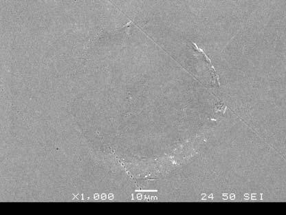
151 260 mw 136

152 390 mw 137

153 390 mw 138

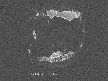
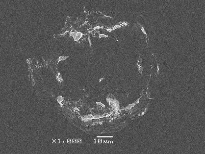
154 520 mw 139

155 520 mw 140

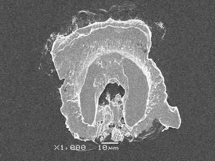
156 650 mw 141

157 650 mw 142

158 Appendix B Wedge Bond Footprints at 50 gf 65 mw 143

159 65 mw 144

160 130 mw 145

161 130 mw 146

162 195 mw 147

163 195 mw 148

164 260 mw 149

165 260 mw 150