Machining - Cutting Tool Life. ver. 1

Transcription

1 Machining - Cutting Tool Life ver. 1 1

2 Overview Failure mechanisms Wear mechanisms Wear of ceramic tools Tool life Machining conditions selection 2

3 Tool Wear Zones chip shear zone cutting tool Crater wear workpiece Flank wear 3

4 Chip / Tool Interface 4

5 Tool Wear (a) (b) (c) Rake Flank (d) (e) 5

6 Tool Wear Zones Crater wear (crater) tool-chip interface predominant at high speeds mitigated by efficient use of carbides Flank wear (wear land) tool-workpiece interface predominant at low speeds 6

7 Gross Fracture Failure Mechanisms High rupture strength needed pure WC - 200,000 psi (1.4 GPa) Al 2 O 3 +TiC - 125,000 psi (0.86 GPa) Transverse rupture strength max. tensile stress at failure of 3 pt. bending 7

8 Failure Mechanisms Gross Fracture Plastic deformation resistance needed function of temperature tensile strength T( o C) 8

9 Failure Mechanisms Fatigue Abrasion Chemical diffusion and convection Chemical diffusion 9

10 Tool Wear Mechanisms Low speed High speed Very high speed Mechanical properties Chemical diffusion and convection Chemical diffusion 10

11 Wear at Low Speeds Mechanical Properties flow induced crack nucleation and growth micro fracture fatigue abrasion Al 2 O 3 at all speeds cutting steel and Ni 11

12 Wear at High Speeds - Chemical Diffusion and Convection Interphase Chip Chip flow Tool atoms Tool 12

13 Chemical Diffusion and Convection Tool dissolves directly into chip Convection - chip sliding on surface transition between sliding and sticking begins maximum heat generation point moves away from tool tip Net flow of material away from interface 13

14 Wear at High Speeds Carbides - super alloys, hard steels Al 2 O 3 - Ti Carbides, nitrides - steels CBN - steels 14

15 Wear at Very High Speeds - Chemical Diffusion Chip Chip flow Interphase Tool atoms Tool 15

16 Chemical Diffusion Transition from sliding to sticking moves from the nose finally sticking occurs everywhere Boundary layer builds up no convection directly from tool to chip only chemical diffusion through boundary layer of chip material 16

17 Wear at Very High Speeds Carbide, diamond - Ti at all speeds CBN - super alloys, hard steels 17

18 Dissolution Controls Wear Tool atoms diffuse up and are swept away by the chip at high temps. Chip Chip flow Tool atoms Tool 18

19 k = Wear Velocity (v wear ) v wear kcv c = equilibrium solubility v y = bulk velocity of chip at chip-tool interface D = chemical diffusivity c y Molar volume of Molar volume of kd = concentration gradient y tool material ( V chip material ( V tool chip ) ) c y 19

20 Wear Velocity Very difficult to determine from first principles Estimate from experiments 20

21 Bulk Velocity - Ex. 1.1 v wear (HfC in Fe) 0.61 mm/min k = V tool (HfC) / V chip (Fe) = cm 3 /mole 7.11 cm 3 /mole = 2.12 c HfC 2.75 x 10-5 v wear 0.61 mm/min = 2.12 x 2.75 x 10-5 x v v(bulk velocity) 10,500 mm/min 1 cm/min 21

22 Relative Wear Rates v v wear wear 1 2 k k 1 2 c c 1 2 V V 1 2 V V chip chip c c 1 2 V1c V c Need solubilities to solve: can be looked up 22

23 Relative Wear Rate - Ex. 2-1 HfC vs. TiC in contact with steel (Fe+C) at 1600 K Example to show method 23

24 Relative Wear Rate - Ex. 2-2 HfC in contact with steel (Fe+C) G HfC G m Hf G m C G = free energy of formation G HfC m G Hf m G C = affinity of Hf for C = affinity of Hf for Fe = affinity of C for Fe Josiah Willard Gibbs

25 Gibbs A little history Gibbs entered Yale University at the age of 15 graduating, in 1858, at the age of 18. He then entered the new Yale graduate school earning the first PhD in engineering in the United States, completed in Gibbs' PhD thesis was On the Form of the Teeth of Wheels in Spur Gearing. In 1871, two years after returning from a study abroad at various universities in Europe, Gibbs became Yale's first professor of mathematical physics. 25

26 Relative Wear Rate - Ex. 2-3 G m i G xs i RT ln c i xs Gi RT lnc i c = concentration = excess free energy (enthalpy) of mixing = entropy of mixing x T =(T S i ) T = absolute temperature (K) R = gas constant = 2 cal/mol/k 26

27 Relative Wear Rate - Ex. 2-4 G HfC = -49,000 cal/mole G xs Hf RT ln c Hf G xs C RT ln c C c Hf = c C for HfC -49,000 = -2,100 + RT lnc Hf + 7,600 + RT lnc C 27

28 Relative Wear Rate - Ex , ,100-7,600 = 2 x 1600 (lnc Hf + lnc C ) = 4 x 1600 x (lnc Hf ) lnc Hf = c Hf = 2 x 10-4 = c HfC 28

29 Relative Wear Rate - Ex. 2-6 G TiC 39,500 cal / mole G xs Ti 6,900 cal / mole G xs C 7,600 cal / mole lnc TiC G TiC xs GTi G 2 R T xs C 29

30 Relative Wear Rate - Ex ,500 6, ,600 lnc TiC 6.28 c TiC

31 Relative Wear Rate - Ex. 2-8 V V HfC TiC c c HfC TiC HfC has 13% of the wear rate of TiC when cutting steel. 31

32 Relative Wear Rate - Ex. 2-9 TiC wears much less than calculated because it forms an oxide layer with oxygen from the steel being cut. TiC predicted = 10.6 TiC actual = 2.75 TiC 0.75 O 0.25 = 2.61 G TiO < G TiC 32

33 Concentration - General Expression c A x B y G exp A x B y x G xs A xs y G B RT x ln x y ln y x y RT 33

34 Nickel Alloys Similar calculations not too accurate. Nickel forms more stable intermetallic compounds than iron. 34

35 Affinity Estimation - xs Gi Free energy of formation of intermetallic compounds Good indication of stable compounds xs is very negative Gi Get from: G of intermetallic Phase diagram 35

36 Affinity Estimation - Ex. 3-1 TiC and stainless steel (Fe, C, Ni) Phase diagram of Ni-Ti: 1726K Solid solution 1653K 1560K Ni+Ni 3 Ti Ni 12.5% Ti 36

37 Affinity Estimation - Ex. 3-2 Ni 3 Ti: H = enthalpy of formation = -33,500 cal/mole G = H - T S G H = -33,500 cal/mole 0 37

38 Affinity Estimation - Ex. 3-3 Equilibrium between stainless steel and intermetallic: ΔG ΔG sol m Ti of Ti in SS ΔG Ni ( per mole of Ti) 3Ti per mole Ti ΔG per mole Ti Ni 3 Ti xs ΔG Ti RT ln c 33, 500 Ti cal/mole c Ti = from phase 1560K 38

39 Affinity Estimation - Ex. 3-4 G xs Ti 6,500 33,500 cal / mole G xs Ti 27,000 cal / mole This is the value for Ti in Ni. This number is different than -6,900 cal/mole, for Ti in Fe. 39

40 Wear of Ceramics (low speed) Ceramics are very stable chemically c (dissolution) is small c y (diffusion) is small Mechanical wear is left as mechanism flow, fracture, fatigue thermal, mechanical 40

41 Wear of Ceramics T cutting > 0.5 T m (Al 2 O 3 ) (in K) Al 2 O 3 is quite ductile Delamination theory voids join to form cracks which form sheet-like wear plates (in areas of intimate contact) void crack 41

42 Wear of Ceramics Outside areas of intimate contact intermittent contact thermal cycles low thermal expansion, low modulus mechanical (stress) cycles 42

43 Tool Wear and Life Tool life depends on application Total destruction rough cutting - surface damage at failure Fixed value of flank wear easy to measure, tools fail by cratering at high speeds (0.38 mm) for finish cuts (0.76 mm) for rough cuts 43

44 Tool Wear and Life Surface finish Cutting rate - band sawing constant feed force cutting rate decreases as tool dulls Excessive torque - drilling breakage 44

45 How to affect tool life? In tests, T q -n T = tool life q = temperature n =

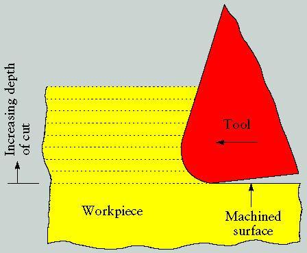
46 How to affect tool life? Reduce temperature hard to do Cutting fluids do not penetrate to interface - small effect Can adjust V = cutting speed (very sensitive) f = feed rate (sensitive) determines surface finish d = depth of cut (not sensitive) 46

47 Taylor s Equation VT n = C V = cutting speed T = tool life n, C = Taylor constants (empirical) C log V n Frederick W. Taylor log T 47

48 F.W. Taylor s Contributions Metal cutting Time / motion studies Led to Congressional inquiry and banning of stop watch use by civil servants ( ) Design of shovels Scientific management 48

49 Extended Taylor s Equation f = feed rate VT n f m =C For high speed steels: V T 0.24 f 0.45 = 23 T= C V -4.2 f

50 Taylor s Equation - Ex. 4-1 Derive Taylor s equation from data speed (V) (sfpm) [m/s] tool life (T) (min) 600 [3.1] [3.6]

51 Taylor s Equation - Ex. 4-2 VT sfpm) = VT sfpm) 700(12.2) n = 600(19.95) n 700/600 = = (19.95/12.2) n n 0.31 C = 600 x VT 0.31 =

52 Choosing Machining Conditions Pick maximum possible depth of cut Take maximum feed rate subject to: surface finish (see next slides) power limitations of machine If you re power limited, are chips breaking? Chips break at f > /min (0.13 mm/min) Pick cost optimum speed 52

53 Tool Marks 53

54 Surface Marks (a) (b) Surfaces produced on steel by cutting, as observed with a scanning electron microscope: (a) turned surface and (b) surface produced by shaping. Source: J. T. Black and S. Ramalingam. 54

55 Roughness f Roughness AA r 2 f Roughness t 8r f = feed r = nose radius AA = arithmetic average t = peak-to-valley f r 55

56 Summary Failure mechanisms Wear mechanisms Wear of ceramic tools Tool life equations Machining conditions selection 56

57 57