Prioritizing Water-Quality Improvement Efforts on Agricultural Lands Using LiDAR Elevation Data

Transcription

1 Prioritizing Water-Quality Improvement Efforts on Agricultural Lands Using LiDAR Elevation Data Aaron Ruesch and Theresa Nelson Wisconsin Department of Natural Resources WLWCA March 11, 2014

2 Outline WLWCA 2013 TMDLs Erosion Analysis Methods Erosion Analysis Results

3 Acknowledgements Adam Freihoefer Ann Hirekatur Sarah Kempen

4 Model Data Requirements Data Requirements Level of Effort Targeted Basins Targeted Fields

5 Leverage Existing Data Topography Soils Hydrography CAFO NM BMPs Outfalls Barnyards Monitoring

6 Erosion Vulnerability Analysis Tool Low Medium High

7

8 Impaired Waters

9 TMDL Total Maximum Daily Load Established under the Clean Water Act The maximum amount of a pollutant that a waterbody can receive and still safely meet water quality standards Allocations

10 TMDL Purpose Current Pollutant Load Does not meet water quality standards Total Maximum Daily Load Meets water quality standards

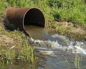
11 Point Sources Nonpoint Sources Pollutant Sources Non-MS4 Stormwater Construction Rill, Gully, & Bank Erosion Agricultural Runoff Barnyards Industrial Waste Municipal Waste

12 TMDL Process Monitoring Conceptualization Modeling Allocations Implementation TMDL

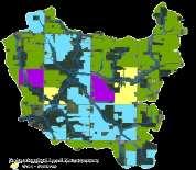
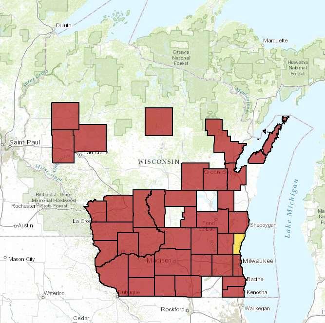
13 TMDLs Statewide

14 TMDL Results Total Phosphorus (lbs/acre/year)

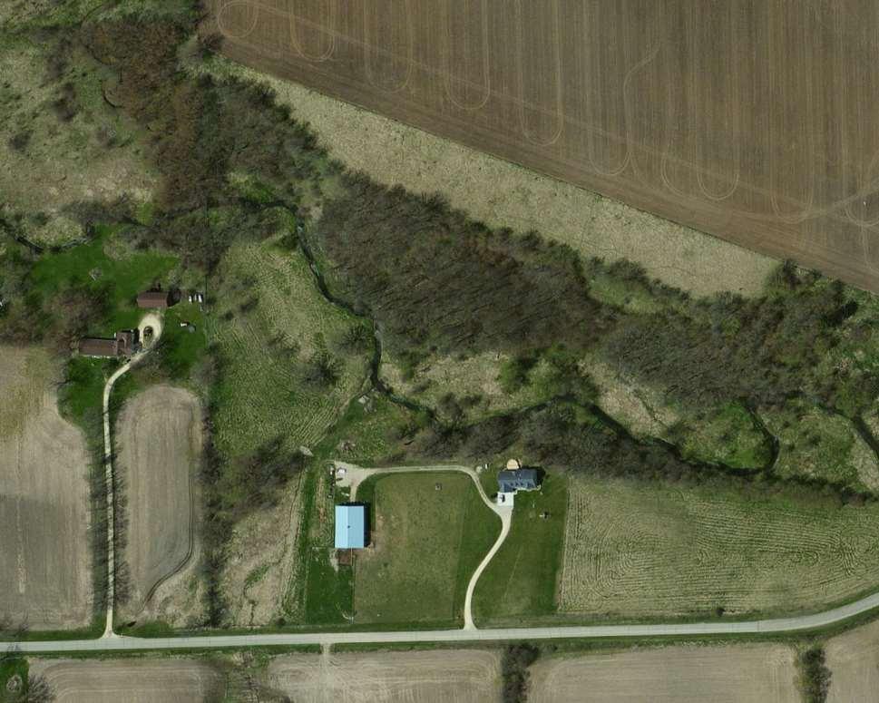
15 Kankapot Creek Watershed? 23 square miles 187 farms 1,129 fields

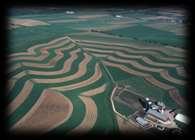
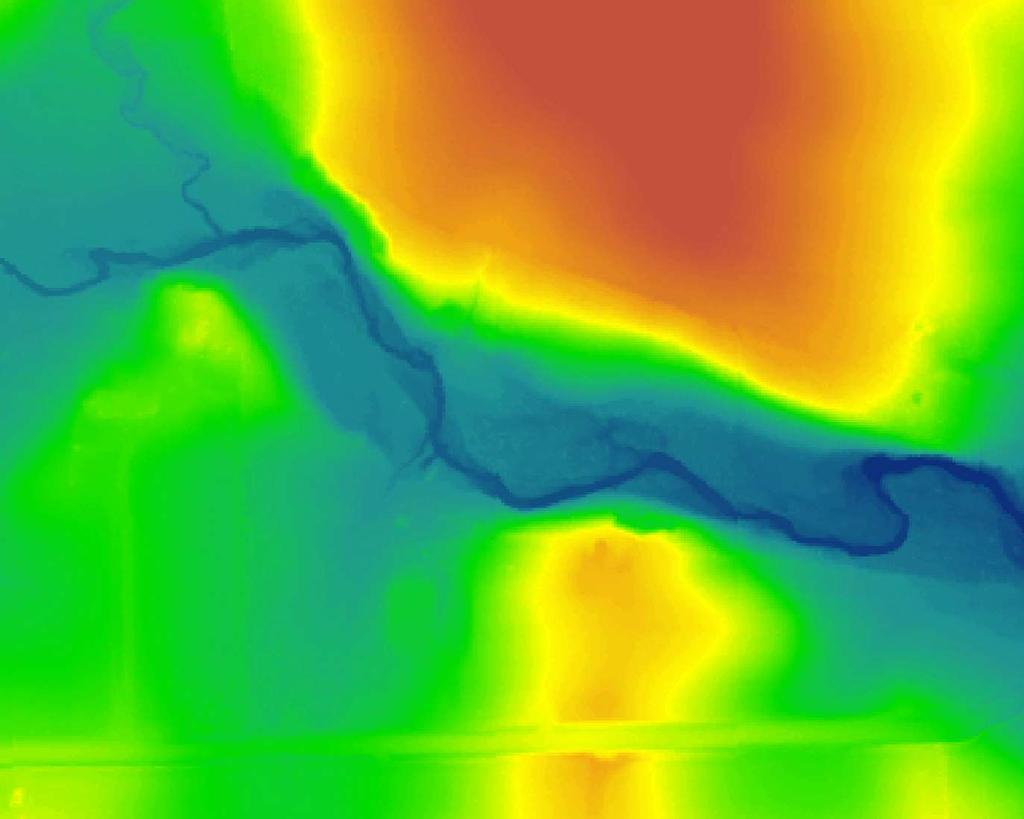
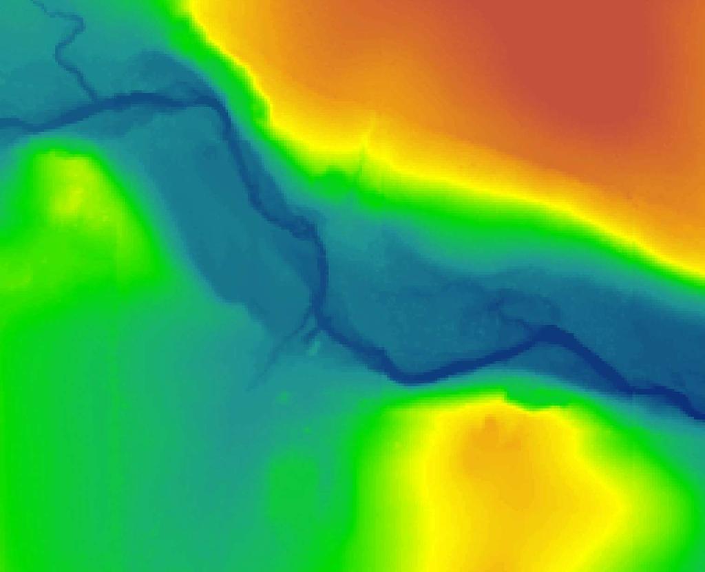
16 LiDAR = Topography. It can help us identify erosion! JOURNAL OF SOIL AND WATER CONSERVATION

17

18 5 5 5 feet Elevation (feet)

19 Total Phosphorus Concentration (mg / L) 0.45 Correlation between Erosion and Phosphorus Total Suspended Sediment Concentration (mg / L)

20 3 model components 1. Total soil loss Based on the Universal Soil Loss Equation (USLE) 2. Potential for gully formation Gullies contribute and deliver sediment 3. Identification of internally draining areas Areas that will not contribute runoff for a typical storm event

21 3 model components 1. Total soil loss Based on the Universal Soil Loss Equation (USLE) 2. Potential for gully formation Gullies contribute and deliver sediment 3. Identification of internally draining areas Areas that will not contribute runoff for a typical storm event

22 3 model components 1. Total soil loss Based on the Universal Soil Loss Equation (USLE) 2. Potential for gully formation Gullies contribute and deliver sediment 3. Identification of internally draining areas Areas that will not contribute runoff for a typical storm event

23

24

25

26 Sheet and Rill (USLE) Potential gully

27

28

29

30 Data prep

31 Data prep Geolocated culverts

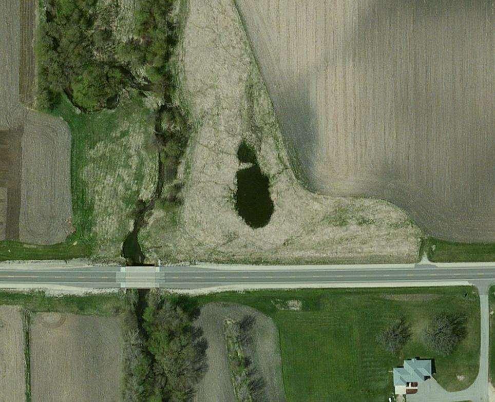
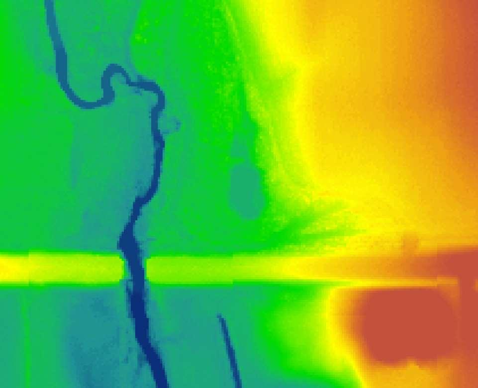
32 The Solution Generalize topography and cut through digital dams

33 The Solution Generalize topography and cut through digital dams

34 Identification of internally draining areas Big storm event LANDSCAPE PROFILE Stream Elevation

35 Identification of internally draining areas CURVE NUMBER METHOD runoff = f(precip, landuse, soils)

36 Identification of internally draining areas Runoff Volume, V R Sink Volume, V S

37 Identification of internally draining areas Runoff Volume, V R Sink Volume, V S Vs Vr, Internally drained Vs < Vr, Not internally drained

38

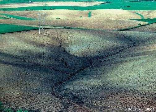
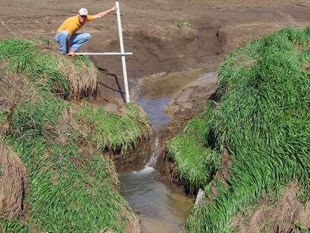
39 How do we automate erosion identification? Potential for gully formation Gullies facilitate erosion and delivery of sediments

40 SPI = Stream Power Index = f(slope, catchment area)

41

42 Small gully BIG gully Estimated gully

43 How do we automate erosion identification? Total soil loss 1. Based on the Universal Soil Loss Equation (USLE)

44 Universal Soil Loss Equation A = RK(LS)CP Rainfall erosivity

45 Universal Soil Loss Equation A = RK(LS)CP Soil erodibility

46 Universal Soil Loss Equation A = RK(LS)CP Slope/ Slope-length

47 Universal Soil Loss Equation A = RK(LS)CP Cover factor

48 Universal Soil Loss Equation A = RK(LS)CP Practice factor

49 Universal Soil Loss Equation A = RK(LS)CP

50 Universal Soil Loss Equation A = RK(LS)CP Constant Constant A = K(LS)C

51 Universal Soil Loss Equation A = RK(LS)CP Constant Constant A = K(LS)C SSURGO soils DEM Cropland data layer

52 Universal Soil Loss Equation A = K(LS)C SSURGO soils DEM Cropland data layer Cover factor varies from years to year

53 What are farmers growing? Corn Soybean Corn Corn Soybean C-C-S-C-C, C-S-C-S-C, S-C-C-S-C, C-C-C-C-S, S-S-S-S-C = Cash Grain Rotation

54 What are farmers growing? Crop Rotation Continuous Corn Cash Grain Dairy Pasture/Hay/Grassland Not enough data

55 What are farmers growing? C-factor Not enough data

56 How are we doing? R 2 = 0.6

57 How are we doing? Labor intensive R 2 = 0.6 Quick, easy, cheap

58

59

60

61 Overall erosion score Erosion Score High Medium Low

62 Where are the animals? Animal lots

63 Which fields are near surface water pathways? Minimum Distance On stream Far Away

64 Where are farmers already working to curb erosion? Grassed Waterway Contour cropping

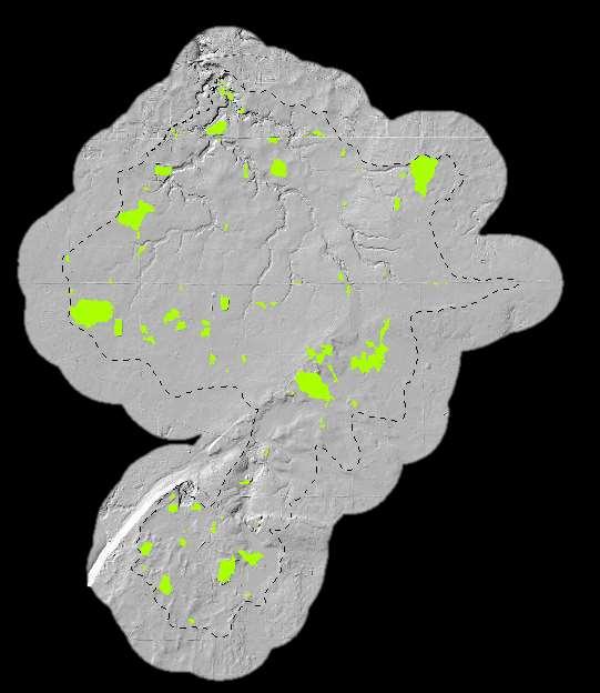
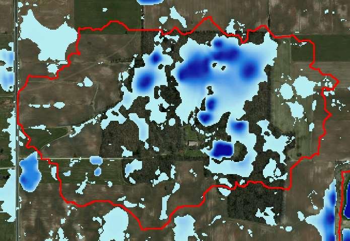
65 Where can we restore wetlands? Potentially restorable wetlands

66 Putting the Pieces Together LEGEND High Erosion Score Non-contributing areas Pot. Restorable Wetlands Distance from animal lot to stream ft > 300 Crop Rotation Continuous Corn Cash Grain Dairy Pasture/Hay/Grassland Not enough data

67 Simple GIS tools for distribution to county staff

68

69 Conclusions Easily available LiDAR data allows for more detailed analysis Some analyses, like locating internally draining areas require data with data at least as fine as typical aerial LiDAR We can do a lot with less effort More efficient use of time and money

70 Questions?