CGE models and land use

Transcription

1 CGE models and land use Renato Rosa FEEM Prague

2 Outline Land use change in current CGE A very simple approach More refined approaches GTAP-AEZ CGE coupling with a land use model 1

3 Land used modelling in current CGE (GTAP) Forest Products (Logging Sector) Agriculture Crop Production Land Competition between Crops Livestock Land competition with crops 2

4 Land used modelling in current CGE (GTAP) Total land is fixed Land is homogenous Land suitability No spatial dimension No land competition between forestry and agriculture (Deforestation, biofuels, forest based carbon sequestration ) ( ) 3

5 4 A very simple approach

6 A very simple approach REDD DATA IIASA Cluster model (Gusti et al. 2008)) Business as usual deforestation rates LACA IIASA Carbon Price Million Tons

7 A very simple approach Business as usual scenario Agriculture/ Pasture Land (2001) IIASA BAU deforestation rates Agriculture/ Pasture Land (2020) Deforested land 2001 (IIASA) Accumulated Deforested land (IIASA) 6

8 A very simple approach Policy Scenario Agriculture/ Pasture Land (2001) Agriculture/ Pasture Land (2020) Carbon Policy Carbon Price Avoided Deforestation Timber modelling follows a similar approach! 7

9 A very simple approach Limits to REDD credits in the ETS market No REDD 5% 10% 15% 20% 25% 30% 50% No Limits CO 2 Price % reduction -6% -12% -17% -22% -27% -32% -50% -83% European Policy Cost (Million US$) ETS without REDD ETS with 10% REDD ETS with 30% REDD ETS with REDD

10 A very simple approach Unlimited use of REDD credits may flood the European carbon market (if this policy is unilaterally undertaken) Limiting the use of REDD credits allows for: Controling the carbon price decrease Provides significant policy cost savings Reduces carbon leakage 9

11 More sophisticated approaches GTAP-AEZ Coupling a CGE model with a global land use model

12 More sophisticated approaches GTAP-AEZ Coupling a CGE model with a global land use model

13 Coupling a CGE model with a global land use model LAND USE MODELS: Geographic Perspective spatial patterns of land, land use types based on land suitability Economic perspective focus on drivers of land use change on the side of food production and consumption Integrated models of land use change (KLUM, GLOBIOM )

14 CGE Initially developed for trade analysis Walrasian perfect competition paradigm Interlinked Markets ( )

15 KLUM Global agricultural land use model designed to link the economy and vegetation Maximization of profits under risk aversion Decreasing returns to scale Profitability of a crop is determined by its price and yield

16 Coupling benefits: More geographically explicit representation of land Land is not classified by different productivity

17 Goals: Replace the endogenous land allocation produced by a CGE model based on economic rationales with exogenous information extracted from a land use model (KLUM) Better environmental representation : E.g. Bio-physical heterogeneity of land Geographic location of land.

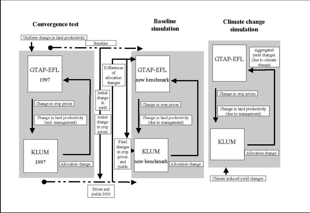
18 Coupling Ideas Exogenous Shock Input GTAP Output Input % Changes in Relative Crop Prices and Land Productivity Iteration until convergence of prices, yields and quantities KLUM Output Input % Changes in quantity of Land Allocated to Different Crops

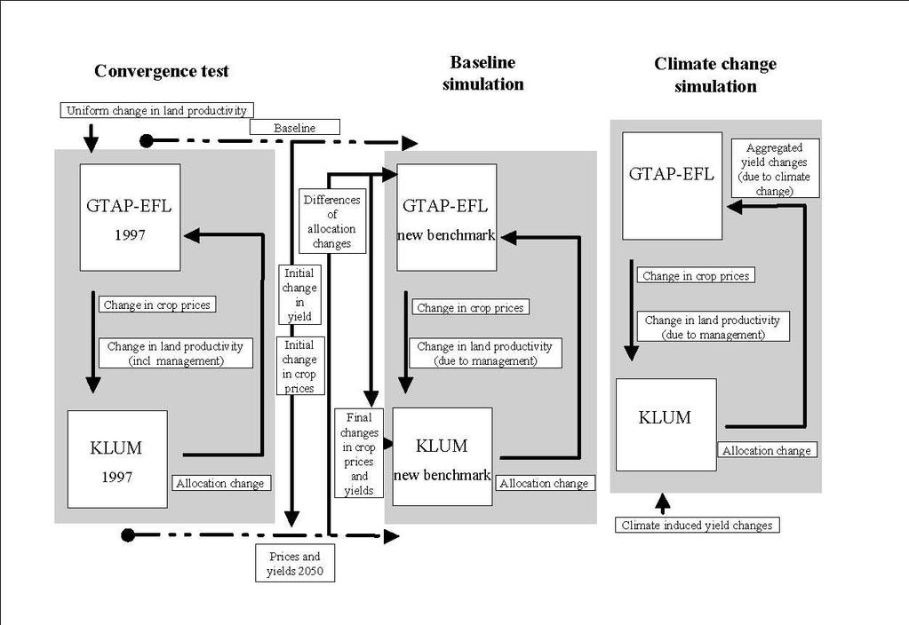
19 Convergence Test

20 Convergence Test Main difficulties Different initial land allocations General constraint imposed by the structure of the CGE model itself. Method Change the responsiveness of GTAP-EFL to changes in land allocation. The key parameter governing this is the sectoral elasticity of substitution among primary factors

21 Convergence Test - Results

22 Benchmarking to 2050

23 2050: CGE Model vs Coupled system: crops production and prices Production Prices Rice Wheat Cereals Veg.& Fruits Rice Wheat Cereals Veg.& Fruits USA CAN WEU JPK ANZ EEU FSU MDE CAM SAM SAS SEA CHI NAF SSA SIS

24 Results and Conclusions The results of standalone simulations generally differ from those of the coupled simulation by some ten up to several hundred percent and show opposite signs for some cases. All this strongly supports the hypothesis that a purely economic, partial equilibrium analysis of land use is biased; general equilibrium analysis is needed, taking into account spatial explicit details of biophysical aspects. Preliminary exercise lot still needs to be done. 23

25 24 and ICES

26 Drivers of Land Use changes 1 Climate: Mean spring-summer precipitation Mean spring-summer temperature Mean spring-summer solar radiation Mean fall-winter precipitation Mean fall-winter solar radiation Mean fall-winter temperature 2 Irrigation 3 Elevation 25

27 - Domain and sub-regions Resolution: 5 x5

28 Spatial module DRIVING FACTORS INITIAL LAND USE Non-spatial module STATISTICAL ANALYSIS CHANGES ON DRIVING FACTORS LAND USE PROBABILITY FOR THE FUTURE NEIGHBOURING ELASTICITY ALLOCATION LAND USE FUTURE DEMAND OTHER FUNCTIONALITIES 27 Modified from Verburg et al., 2002

29 The coupling From the ICES model vector of demands for different land uses (crops and/or timber) consistent with a given social economic scenario/ assumption CLUE ICES Feedback CLUE, given its initial land allocation, spatially allocates the demand

30 LU fractions (area per cell) Wheat A2_T_M B2_T_M

31 Thank you