David M. Rocke Division of Biostatistics and Department of Biomedical Engineering University of California, Davis

Transcription

1 David M. Rocke Division of Biostatistics and Department of Biomedical Engineering University of California, Davis

2 Outline RNA-Seq for differential expression analysis Statistical methods for RNA-Seq: Structure and choices Criteria for comparison of statistical methods Results of three packages on a data set Null performance Source of differences in the results Input data Tests Variance estimation Normalization Conclusions

3 RNA-Seq Gene expression is the transcription of the DNA in a gene into mrna, which (in many cases) is later translated into a protein. We can measure expression of a single gene with PCR or other assays. Gene expression arrays measure expression of many genes simultaneously using spots each of which contains a matching sequence to the gene sequence to be detected. But this can only detect what we already suspected might be there.

4 RNA-Seq For RNA-Seq, the RNA in the sample is reverse transcribed into the corresponding DNA sequence. Then the DNA fragments are sequenced (in an NGS sequencer, usually Illumina ) Each fragment is mapped to the reference genome The data to be analyzed are the number of fragments mapping to each gene in a table where the columns are samples and the rows are genes.

5 RNA-Seq This mapping can be complex We can choose to estimate isoforms or not We can choose how to handle ambiguous reads (omit or spread across genes) We can then use statistical analysis to determine when there is significantly more expression in one condition or another. This may or may not be better than an expression array depending on goals.

6 Analysis of RNA-Seq Data For each gene/exon/isoform (we will say gene from now on), and for each sample, we have a count of fragments mapping to that gene. In principle, we need to test whether the counts from one group are significantly larger than another. Or we may have more than one factor or variable that could be associated. In practice, we may (probably) need to normalize the samples first, and may need to import some information across genes.

7 Existing Methods Existing methods often contain complex combinations or filtering, normalization, transformation, and variance estimation before any statistical tests are performed. The methods are often poorly documented and change rapidly and often substantially between frequent versions, without any push notice. The results of different methods such as DESeq, edger, and voom/limma can differ substantially. It appears that most methods produce large numbers of false positives.

8 Bottomly Data Two inbred mouse strains, C7BL6/6J (10 animals) and DBA/2J (11 animals) Gene expression in striatal neurons by RNA-Seq and expression arrays. 36,536 unique genes of which 11,870 had a count of at least 10 across the 21 samples. This data set has been used in other comparisons First, we compare three methods on this data set. Later we construct data sets where the null hypothesis is true.

9 825 Genes Significant by at least one method 486 by all methods More significant genes by edger Is this greater power or is the test producing false positives?

10 Null Behavior 100 randomly selected subsets of size 6 out of the 10 C7BL6 mice (out of the 210 possible) In each subset, 3 assigned to treatment and 3 to control at random (out of 10 possible divisions). The null hypothesis is on the average true. Given the 11,870 genes with large enough counts, we would expect about 0.1% to be significant at the p = level. We have 1,187,000 tests, so there should be about 1187 rejections for each method

11 Significant at p = Null Hypothesis is True Estimator Observed Expected Over-Rejection DESeq % edger % limma-voom %

12

13 Important Factors These methods share some features but differ in their implementation. All of them treat the data as over-dispersed Poisson, or specifically negative binomial They may use a test based on the negative binomial distribution, but limma-voom uses standard regression/anova with variance-based weights Since sample sizes tend to be small, they all have the possibility to replace the variance estimate from a given gene with a smoothed estimate based on all the genes. Normalization may be needed due to the differing total numbers of reads

14 Factors That May Cause False Positives Normalization procedure Normalization driven by high-abundance transcripts can cause spurious significance of low abundance ones. Variance estimation Many methods borrow strength from other genes to get better variance estimates. This may cause bias Statistical test used Many choices Nature of the data May require filtering

15 Statistical Test Example gene from Bottomly data ENSMUSG C57BL/6J 2, 7, 9, 11, 3, 7, 1, 1, 2, 1 Median 2.5, Mean 4.4, sd 3.75, var DBA/2J 8, 6, 12, 10, 19, 15, 17, 6, 20, 6, 14 Median 12, Mean 12.09, sd 5.28, var 27.89

16

17 Poisson Analysis One of the first ideas was that the counts might be Poisson distributed and that we could use this for statistical tests. In this case, if the null hypothesis was true, then the 21 observations came from the same Poisson distribution with observed mean and with variance also estimated at (Poisson distributions have mean and variance that are equal). This implies that the variance of the mean of the 10 C7BL/6J counts should be 8.429/10 and the variance of the mean of the 11 DBA/2J counts should be 8.429/11 So we can use z = ( )/ (8.429/ /11) = 6.06 to test the difference

18 Poisson Analysis This turns out to be a terrible idea. Frequently, the variance of the data is much larger than the mean. We can call this overdispersion. C57BL/6J Mean 4.4, Variance DBA/2J Mean 12.09, Variance Also, Poisson analysis can be done with one treatment and one control, and any belief that statistical evidence can be gathered with no biological replicates is evidence of terminal delusion!

19 Over-dispersed Poisson Analysis In this case, we estimate the means and the variances from the data using either the negative binomial distribution or simply an over-dispersed Poisson. These yield similar results. In either case, we model the data in such as way that, for a given gene g and /sample i, the count y E( y ig Var( y ) = µ ig ) = µ + c µ 2 2 ig ig ig ig has

20 > summary(glm(y1~strain,family=poisson)) Coefficients: Estimate Std. Error z value Pr(> z ) (Intercept) < 2e-16 *** straindba/2j e-09 *** (Dispersion parameter for poisson family taken to be 1) > anova(glm(y1~strain,family=poisson),test="chisq") Df Deviance Resid. Df Resid. Dev Pr(>Chi) NULL strain e-10 *** First test is Wald test, second is likelihood ratio test. But Poisson assumption is not valid.

21 > summary(glm(y1~strain,family=quasipoisson)) Coefficients: Estimate Std. Error t value Pr(> t ) (Intercept) e-06 *** straindba/2j ** (Dispersion parameter for quasipoisson family taken to be ) > anova(glm(y1~strain,family=quasipoisson),test="chisq") Df Deviance Resid. Df Resid. Dev Pr(>Chi) NULL strain ***

22 > summary(glm.nb(y1~strain)) Coefficients: Estimate Std. Error z value Pr(> z ) (Intercept) e-13 *** straindba/2j e-05 *** (Dispersion parameter for Negative Binomial(5.1558) family taken to be 1) > anova(glm.nb(y1~strain),test="chisq") Df Deviance Resid. Df Resid. Dev Pr(>Chi) NULL strain e-05 ***

23 P-values ( 10 5 ) Wald LR Quasi-Poisson Negative Binomial Both the Wald test and the likelihood ratio test are valid asymptotically. The quasi-poisson and negative binomial should be equivalent asymptotically But in finite samples there can be substantial differences

24 > t.test(y1~strain) Welch Two Sample t-test t = , df = , p-value = alternative hypothesis: true difference in means is not equal to 0 95 percent confidence interval: sample estimates: mean in group C57BL/6J mean in group DBA/2J Similar results to that using the negative binomial.

25 Is the Test Statistic Important? Not so much Simulated negative binomial count data Two groups of 10 Mean 5 and variance 6 10,000 trials Test Reject at 5% Reject at 1% Reject at 0.1% t-test 4.9% 0.90% 0.11% Wilcoxon Test 4.6% 0.74% 0.03% NB Likelihood Ratio Test 5.2% 0.95% 0.13% NB Wald Test 5.7% 1.16% 0.22% 4.8% 5.2% 0.90% 1.11% 0.07% 0.12%

26 Normalization Normalization is commonly used in differential expression analysis with microarrays. Normalization for RNA-Seq is often couched in terms like library size as if we should divide by the total (mapped) fragment count This can be problematic because it depends on only a few genes. Mostly, normalization in RNA-Seq is done with a single constant per sample, though this is unusual with expression arrays

27 Library Size Normalization Using the total fragment count is problematic because highly expressed genes will provide most of the fragments Four genes with expression 10,000, 100, 150, 200 in condition A and 20,000, 100, 150, 200 in condition B. Normalized fragment counts use total fragment counts of 10,450 and 20,450 and can be normalized to 15,450 Normalized fragment counts are 14,785, 148, 222, 296 in condition A and 15,110, 76, 113, 151 in condition B, so upregulation of gene 1 has been turned into down-regulation of the other three. Fold changes are 2.0, 1.0, 1.0, 1.0 before normalization and 1.02, 0.51, 0.51, 0.51 after.

28 Normalization Methods Total count Quantile Normalization of other signal based methods Geometric normalization (Cuffdiff2/DESeq version) For each gene, compute the geometric mean of the total fragment count across libraries Library size is the median across genes of the total fragment count divided by the geometric mean fragment count. In our 4-gene example, the geometric means are 14,142, 100, 150, 200, the ratios for A are 0.707, 1, 1, 1 and for B are 1.414, 1, 1, 1, so the size factors are the medians, namely 1 and 1

29 k fragment count for gene i in library j ij m 1/ m m 1 gi = ki ν = ki ν ν = 1 m ν = 1 s j exp log( ) kij = median i g i Cuffdiff2 first normalizes replicates under the same conditions giving an internal library size of s j Then the arithmetic mean of the scaled gene counts for each gene is used to compute an external library size of η j. This is a possible source of problems, the scale of which is unknown

30 Variance Estimation Many RNA-Seq experiments are small. Small studies have low power Very small p-values are needed to pass the false discovery filter So the default for small studies is no results Suppose two means differ by one standard deviation With 10,000 genes, the Bonferroni level is With two groups of 3, there are ~4df and corresponds to almost 50 standard deviations

31 Variance Estimation If we use tests that reference only the data from the specific gene, then usually variance estimation is not a problem. But with small sample sizes, the power is low, so there is a temptation to improve the variance estimates by smoothing or shrinkage. The variance of a negative binomial increases with the mean in a way controlled by a variance parameter. We can smooth the plot of the sample variance vs. the mean and use the smoothed estimate instead of the per-gene estimate.

32 A Poisson random variable with parameter λ has µ = λ σ 2 = λ A negative binomial random variable can be seen as a mixture of Poissons with varying λ µ = λ σ = λ+ c λ σ / µ = λ + c c s x cˆ = if this is positive 2 x If we smooth a plot of the variance or the square CV or cˆ 2 vs. the mean we obtain an average estimate of c for the given value of µ We can use the individual variance, the smoothed variance, or a compromise

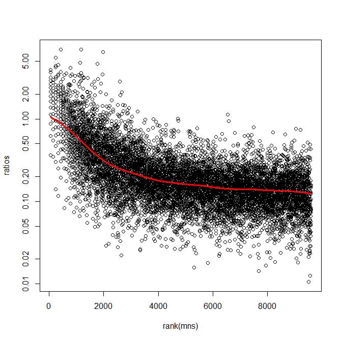
33

34

35 Variance Estimation The sample variance is an unbiased estimate of the population variance A smoothed variance will be biased down or up depending on the data point While this can reduce the MSE of estimating the variance, it may increase false positives and false negatives for tests based on those variance estimates This is a possible source of the differences in results in various methods of analysis.

36 Conclusions Analysis of RNA-Seq data is still in the early stages of development. Existing programs vary substantially in the results and it is unclear which is the most reliable More work is needed that focuses on the fundamental components of analysis, particularly variance estimation and sample normalization.