USE OF SALE CHARTS IN DETERMINING MOMENT AND SHEAR

Transcription

1 APPENDIX C USE OF SALE CHARTS IN DETERMINING MOMENT AND SHEAR FM When a simple horizontal beam is loaded, it deflects, or bends downward, and the horizontal fibers in the lower part of the beam are lengthened (tension) and those in the upper part are shortened (compression). The external forces act to produce a bending moment. The moment of the internal forces (stresses) resisting this bending is called the resisting moment. In Figure C-1, in that part of the beam to the right of section C, the counterclockwise bending moment produced by the external force P and Rr is resisted by the clockwise resisting moment produced by the tensile and compressive stresses in the beam at section C. Within the strength of the material, the resisting moment at any section is equal to the betiding moment at that section. When abeam is designed, the dimensions must be such that the maximum resisting moment that the beam can develop is at least equal to the greatest bending moment that may be imposed on it by the external loads. BENDING MOMENT The following procedures, formulas, and other data are relevant to the determination of maximum allowable bending moment: The bending moment at any section (point) of a beam for an external load in a specific position is found as follows: 1 Determine reactions caused by load in this position. 337

2 2 3 Take either reaction and multiply it by distance of that reaction from section under consideration. From this product, subtract product of each load applied to beam between reaction and section times the distance from that load to section. In Figure C-2, external bending moment at C equals M c = (R L x 20) - (8,000 x 10) = 260,000-80,000 = 180,000 foot-pounds, or M c = 18,000 x 12 = 2,160,000 inch-pounds. This may also be found by taking forces from the right end. The bending moment at any point in a beam due to a moving load varies with the position of the load. For design, it is necessary to know the maximum moment that is caused by the load as it moves across the bridge. Maximum bending moment caused by a single concentrated axle load occurs at center of span when load is at center of span. Maximum bending moment produced by a uniformly distributed load occurs at center of span when distributed load covers entire span. If distributed load is shorter than span, maximum bending moment occurs at center of span when center of load is at center of span. The following formulas are useful in determining maximum bending moments caused by single loads on simple beams: (Concentrated center load P) (Total load W uniformly distributed over span 1) M = w1 2 (Load w per linear foot distributed over span 1) Where M= P= W= w= 1= b= (Load W partially distributed over span 1) Moment in inch-pounds at center of beam Concentrated load in pounds Total distributed load in pounds Distributed load per linear foot in pounds Span in inches Length of load in inches EXAMPLES: What is the maximum bending moment produced in a 20-foot span by a single concentrated axle load of 30 tons? By a total load of 5 tons uniformly distributed over the span (dead load)? By a 30-ton tank that has 147 inches of track? SOLUTIONS: For a single concentrated axle load of 30 tons: Where P= 30 tons (60,000 pounds) 1 = 20 feet (240 inches) = 3,600,000 inchpounds 338

3 FM 5277 For a uniformly distributed load of 5 tons: For a 30-ton tank: = 2,497,500 inch-pounds = 300,00 inchpounds For a series of axle loads on a span, maximum moment may occur under the heaviest load when that load is at the center of the span, or it may occur under one of the heavier loads when that load and the center of gravity of all the loads on the span are equidistant from the center of the span. Further details on computing maximum bending moment produced by two or more loads on a span can be found in engineering handbooks. For the design of military bridges the computation of maximum bending produced by a series of axle loads or that produced by a uniformly partially distributed load, such as a tank, has been simplified by the use of single-axle load equivalents (SALE). The SALE is that single-axle load that, when placed at midspan, will cause the same maximum moment as the maximum moment caused by the actual vehicle. From the formula above for a concentrated center load P, and substituting SALE, we have RESISTING MOMENT Maximum allowable resisting moment that a beam can develop is the product of maximum allowable fiber stress for the material and section modulus of the beam, which is a measure of the capacity of the cross section of the beam to resist bending. Where M is the maximum allowable resisting moment that a beam can develop; f, the allowable extreme fiber stress for the material; and S, the section modulus, their relationship is expressed by the formula M = fs.s depends solely on shape and size of the cross section and f on the material of the beam. For rectangular beams, such as timber stringers, S for I-bems and other structural steel shapes may be found in tables in standard engineering handbooks. Values of S for selected I-beams and WF (wide flange) beams are given in Tables C-1 and C-2 (page 340). The stress f is ordinarily expressed in pounds per square inch, and band din inches, giving M in inch-pounds. Values of f will vary according to type of stress and type of material. For this text and the majority of field design, values as given in the next section are used. For example, if the extreme allowable fiber stress (f) in bending of the wood in a rectangular beam 6 by 12 inches is 2,400 pounds per square inch, then the maximum allowable bending moment that beam can resist is: = 345,600 inch-pounds. 339

4 The following procedures, formulas, and other data are relevant to the determination of maximum allowable shearing stress: For beams supported at both ends, the shear at any section (point on the beam) is equal to the reaction at one end of the beam minus all the loads between that end and the section in question. To calculate maximum shear, it is necessary to find the position of the loads that produces the greatest end reaction. This usually occurs when the heaviest load is over one support. In timber we find that because of the layer effect of the grain, the stringers are weaker horizontally along the member. But the stress numerically equal to the horizontal direction is numerically equal to the vertical direction, so design is on the basis of the stress in the vertical direction. In military bridge design a shear check must be made if the span length in inches is less than 13 times the depth of the stringer. SHEAR AND SHEARING STRESS Any load applied to a beam induces shearing stresses. There is a tendency for the beam to fail by dropping down between the supports (Figure C-3 (A)). This is called vertical shear. There is also a tendency for the fibers of the beam to slide past each other in a horizontal direction (Figure C-3 (B)). The name given to this is horizontal shear. The average intensity of shear stress (horizontal and vertical) in a beam is obtained by dividing maximum external shear by cross-sectional area of the beam. However, shear is not evenly distributed throughout the beam from top to bottom, so maximum shear intensity is greater than the average. Maximum shear intensity occurs at the midpoint of the vertical section. 340

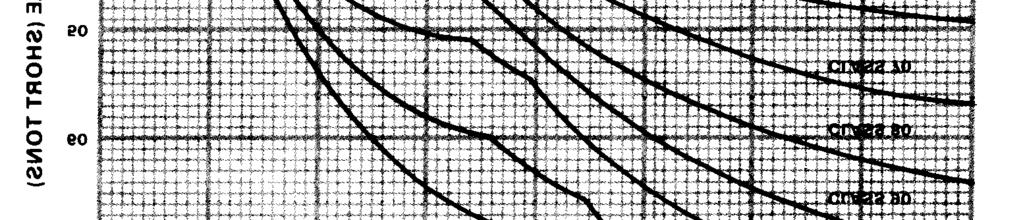
5 For a rectangular section, maximum horizontal shear intensity equals 3/2 times average intensity, or Where S h = V= b = d= maximum shear intensity (unit shear stress) induced in the beam, in pounds per square inch maximum shear, in pounds breadth of beam, in inches depth of beam, in inches Over short spans where shear rather than bending may control, beams warrant special means of analysis. In computing maximum horizontal shear intensity, use the formula given above. In determining V for use in this formula, neglect all loads within a distance equal to or less than the beam height from either support, and place the design moving load at a distance three times the height of the beam from the support. For a circular section, maximum horizontal shear intensity equals 4/3 times average intensity, or Where d = s diameter of beam, in inches CLASSIFICATION OF VEHICLES AND BRIDGES The purpose of this paragraph is to outline office and field procedures for classifying vehicles and bridges in accordance with the vehicle and bridge classification system and to explain the field design of simple bridges. It explains vehicle and bridge classification procedures in sufficient detail to enable engineers who are familiar with the classification system to determine the proper classification of vehicles and bridges. It also explains how to select stringers for simple-span bridges and to design the substructure using timber trestle intermediate supports. STANDARD CLASSES A group of 16 standard classes ranging from 4 to 150 has been established at the intervals shown in Figure C-4 (pages 343 and 344). For each of the standard classes two hypothetical vehicles are assumed: a tracked vehicle whose weight in short tons is the standard class number, and a wheeled vehicle of greater weight which induces about the same maximum stresses in a given span. For example, in standard class 4 the tracked vehicle weighs 4 tons, the wheeled vehicle 4.5 tons; in class 8, 8 tons and 9 tons, respectively. The hypothetical vehicles and their characteristics are shown in Figure C-4. Although these vehicles are hypothetical, they approximate actual United States and United Kingdom army vehicles. For each standard class both a moment class curve and a shear class curve are drawn. These curves are determined by computing the maximum moment and maximum shear induced in simple spans by the two hypothetical vehicles for each standard class, converting these values to single-axle-load equivalents (SALE), in short tons, and plotting the SALE against the simple-beam span in feet. The envelope curve is then drawn through the maximum moment and shear values as shown in Figures C-5 and C-6 (page 345). The standard class curves are shown in Figures C-7 through C-12 (pages 345 through 348). In computing maximum moment and shear, space the vehicles at normal convoy spacing, with an interval of 30 yards from the tail of one vehicle to the front of the next vehicle. SPECIFICATIONS The basic assumptions and specifications used here for design and capacity estimation data are as follows: As regards bending stress: steel 27,000 pounds per square inch; timber 2,400 pounds per square inch. As regards shear stress: structural steel sections 16,500 pounds per square inch; steel pins and rivets 20,000 pounds per square inch; timber 150 pounds per square inch. As regards impact: steel 15 percent of live load moment; timber none. As regards the lateral distribution factor theoretically, two stringers are twice as strong as one, four are twice as strong as two, and so on; actually, this is true only if 341

6 each stringer carries an equal share of the As regards the distance between road total load. A stringer directly under a contacts of vehicles following in line: 100 wheel load is more highly stressed and feet. carries a greater portion of the load than those farther to the side. Because of this OFFICE DETERMINATION nonuniform lateral distribution of a wheel Use the following method to determine veload among stringers, the total width (or hicle class number in the office: number) of stringers required to carry a particular load is greater than the total 1 Compute the maximum moment produced width (or number) that would be required by the vehicle in at least six simple spans if all stringers carried an equal share of of different length. the load. This requires an increase in stringer width (or number of stringers) 2 Convert maximum moment to SALE and is expressed as a ratio called lateral using the formula, distribution factor. For design of two-lane military bridges with vehicles on the in which M = maximum moment in foottons, and L = span length in centerline of each lane, the factor is 1.5. feet. As regards roadway widths: a minimum clear width between curbs of 13 feet 6 inches for single-lane bridges and 22 feet for two-lane bridges. 3 Plot SALE against corresponding span length Draw curve through the points plotted. This is the moment class curve for the vehicle. Superimpose the curve over the standard class curves for moment (Figures C-7, C-8, and C-9). Determine the class of the vehicle by the position of the vehicle class curve with respect to the standard class curves. Round off any fraction to the next larger whole number. Repeat the last three steps for maximum shear, using the formula, SALE = shear. The class of the vehicle is the maximum class determined from either the moment or shear curve. In most cases, moment will govern. 342

7 343

8 344

9 345

10 346

11 347

12 EXAMPLES: Single vehicle Figure C-13 shows the moment curve for a 2 1/2-ton, 6x6 dump truck superimposed on the standard class curves. From the figure 348 it is seen that the curve for this vehicle lies between the class 4 and the class 8 curves and from its position with respect to these curves the vehicle is class 8. Combination vehicle over class 40 Figure C-14 shows the moment curve for a M26A1 tractor with transporter M15A1, loaded, superimposed on the standard class curves. From the figure it is seen that at a span length of 100 feet the superimposed curve crosses the standard class 70 curve and begins to level off. It does not cross the class 80 curve. From its position with respect to the standard class curves, the class of the vehicle is 77. Figure C-14 shows that the vehicle has lower classes at shorter span lengths. At a span length of 70 feet, for example, the vehicle s class curve crosses the standard class 60 curve, and for this span the class of the vehicle is 60. The other classes of the vehicle for shorter span lengths are similarly determined by inspection of the curves, and this information is placed on a cab plate. The section of the cab plate for this vehicle, loaded, shows the class restrictions for the various spans, listed in Table C-3. FIELD DETERMINATION If time, information, or a qualified engineer is unavailable, and the office methods cannot be used, substitute one of the following methods: Compare characteristics such as dimensions, axle loads, and gross weight with characteristics of the hypothetical vehicles shown in Figure C-4. EXAMPLE: An unclassified wheeled vehicle has a gross weight of 27 tons and a length of about 27 feet. By interpolation in Figure C-4, it is class 23. If, however, because of

13 axle spacing and weight distribution the maximum single-axle load for this vehicle is 12.5 tons (greater than Figure C-4 shows as allowable for class 23), the maximum single-axle load is used as the classifying criterion. By interpolation in the maximum single-axle load column (Figure C- 4), the vehicle is then class 26. Compare the characteristics of an unclassified vehicle with those of a similar classified vehicle. EXAMPLE: An unclassified single vehicle has three axles, is about 166 inches long, and weighs about 8 1/2 tons. By comparison with a standard 2 1/2-ton truck 6x6-LWB, which weighs 8.85 tons, it is class 8. Compare the ground-contact area of an unclassified tracked vehicle with that of a classified tracked vehicle. Tracked vehicles can be assumed to be designed with about the same ground pressure. EXAMPLE: An unclassified tracked vehicle has a ground contact area of about 5,500 square inches. By comparison with an M4 tank, which has a ground contact area of 5,444 square inches, it is class 36. Compare the deflection in a long steal span caused by an unclassified vehicle with the deflections caused by classified vehicles. In this method the span must be at least twice as long as the vehicles and the vehicles must be placed for maximum deflection. Measuring apparatus must be accurate to at least one thirty-second of an inch. EXAMPLE: Select two vehicles of known class which are estimated to bracket the unknown vehicle class. Measure the deflections of a long steel span when loaded individually by each of the three vehicles. Move each vehicle on the span three times and read the deflection. Then average the three readings. 349

14 Deflection Vehicle Class (average of three loadings) A /32 in, or 2.406in B /16 in, or in C unknown 2 3/32 in, or in Class is considered proportional to deflection so Unknown class = lower class + (Upper class lower class) x deflection of unknown class minus deflection of lower class Deflection of upper class minus deflection of lower class = = 53.31, or class