Habitat loss and degradation

Transcription

1 Book reading that covers lectures up to the test Habitat loss and degradation PVA: Essay 12.2 (and adjacent text) Loss: Irreversible damage of a habitat Species invasion: p (Case study 9.4 is informative on biological control), no other boxes or essays. Some parts in this chapter were not discussed in class. Degradation: permanent or temporal degradation (reduction of its function) of a habitat Transformation from one type into another one Overexploitation: p , p p !! (no Box or Essays) Habitat degradation: p , Essay 6.1 Habitat fragmentation: p , Essay 7.1, Box 7.1 Loss of rain forest Source of 1620, 1850, and 1920 maps: William B. Greeley, The Relation of Geography to Timber Supply, Economic Geography, 1925, vol. 1, p Source of TODAY map: compiled by George Draffan from roadless area map in The Big Outside: A Descriptive Inventory of the Big Wilderness Areas of the United States, by Dave Foreman and Howie Wolke (Harmony Books, 1992)hi. Loss of wetlands

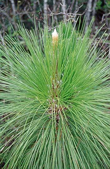
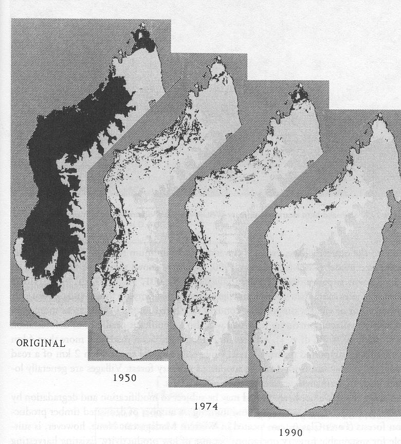
2 Longleaf pine forests degradation Fringed prairie orchid loss transformation Process of fragmentation Native habitat Transformed habitat Gap formation Time Western Madagascar, Warwickshire, England

3 US Pacific Northwest, Willamette National Forest, Oregon, 1979 Major changes in fragmented habitats Habitat shredding Size: Isolation: Edge/interior: decreases increases increases natural shreds Native habitat Transformed habitat Shredding Patchy Habitat fragmentation isolated patches (island biogeography) fragments have small area and (typically) a center and an edge Habitat shredding connected to good habitats (theory?) consists mostly of edge

4 and Heterogeneity and Heterogeneity and Heterogeneity and Heterogeneity Quantifying fragmentation Shannon-Wiener variant Shannon-Wiener index Shape complexity Proximity index spatial statistics H = k p k ln p k ln s p k = frequency of map class k s = total number of map classes Range of H* is scaled between 0 and 1 0 low diversity and uneven habitat classes 1 high diversity and even habitat classes

5 Complexity of habitat patches Comparison of such indices! log A d log P A = area of a patch P = perimeter of a patch d = fractal dimension Shannon - Wiener ignores shape (interior versus edge) Complexity measures only within patch class, but takes edge versus interior into account Simple indices often do not tell the (whole) truth d is found by regression and then scaled between 1 and 2. A value of two means more edge per patch and a value of 1 is equivalent with circular patches. Roads increase invasives Importance of roads Wilderness designation Spread if invasive species Settlement/Development Wilderness designation Is the area 5,000 acres in size or larger? Or a roadless island? Does the area generally appear to be natural and is human presence relatively unnoticeable? Does the area offer the opportunity for primitive and unconfined recreational activities like camping, hiking, and skiing? Does it provide opportunities for solitude? Does the area contain features of ecological, geological, scientific, educational, scenic, or historical significance? total = 106,402,582acres

6 Effects of smaller patches Effects of isolation Effects of fragmentation on species: small patches and isolation Genetic drift Inbreeding Heterozygosity Population size Demographic stochasticity Migration, gene flow Colonization / Extinction Diversity Area effect, distance effects (Island biogeography theory) Area effect "Demographic stochasticity Distance effect!patch size!population size Extinction!Patch isolation " Gene flow Migration "Extinction risk!colonization "Genetic drift, "inbreeding,!heterozygosity "Colonization "Patch occupancy!local adaptation,!fst,!inbreeding, "heterozygosity!diversity "Diversity "Metapopulation Relaxation = reduction in diversity of a patch after fragmentation from old equilibrium number of species to new equilibrium number. Relaxation: adjusting to a lower level of diversity after isolation Coyotes Wolves Elk Coyotes Pronghorn Elk Plants Habitats that are fragmented will adjust to a lower level of diversity Islands that were once connected to the mainland will adjust to a lower level of diversity Islands that never were connected to a mainland will build up diversity Pronghorn Plants

7 Effects of smaller patches Effects of isolation Diversity!, Extinction " Effects of smaller patches Effects of isolation Diversity!, Extinction " Edge effects Edge effects = edges of habitat are not the same as interior of habitat (biotic and abiotic differences) Forest Edge effects Field Field Forest edge Forest Field The smaller the patch, the more edge relative to interior Edge effects = edges of habitat are not the same as interior of habitat (biotic and abiotic differences) 1 Ha!!! 10 Ha!!! 100 Ha Edges have: more light 100% edge 48% interior 53% edge If edge width is 50 m 81% interior 19% edge higher temperature less moisture different species higher extinction rates

8 None of 16 species breed Effects of smaller patches Effects of isolation Diversity!, Extinction " 6 of 16 species breed Edge effects Species composition changes, Extinction " Secondary Extinctions Biological Dynamics of Forest Fragments (BDFF) Brazilian Amazon Extinctions resulting from other extinctions Initiated in 1979 by WWF and INPA

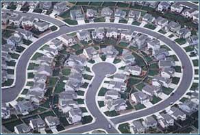
9 Fragment sizes: 1, 10, 100, 1000 Ha; Plus continuous forest Summary of BDFF edge effects: Abiotic variables Biotic variables Decrease in species richness of birds, some! insects, primates, bees, and termites Increase in species richness of small!mammals, amphibians, and butterflies Changes in composition of communities of! butterflies and small mammals Plots are square with side: 100m, 316m, 1000m, 3162m Landscape context Native habitat Transformed habitat Forest fragmentation project in Brazil Landscape context Effect of urbanization Study of e#ects of urban land on reserves: 66 study plots in four grassland types Shortgrass steppe Shortgrass steppe Mixed grass prairie Tallgrass prairie Hayfields

10 Mixed grass prairie Tallgrass prairie Hayfields Hispid pocket mouse Grasshopper sparrow Abundance index Measure of landscape context Landscape suburbanized (%) Urban index Bock et al. 2002, Conservation Biology Haire et al. 2000, Landscape and Urban Planning

11 What do we know for sure? Harrison and Bruna 1999 Species in fragmented habitats are vulnerable to extinction Rate of extinction versus park area (Newmark 1995) Medium-large mammals of landscape as a cause for genetic subdivision of bank vole populations. Gabriele Gerlach and Kerstin Musolf Conservation Biology 14 (2000) 1 10 We studied the barrier effects of various roadways on genetic subdivision of bank vole (Clethrionomys glareolus) populations. Allele frequencies, genetic variability, and genetic distances of natural populations were calculated based on polymorphism of 7 microsatellite markers. We compared bank vole populations in control areas without such barriers with animals from both sides of a country road, a railway, and a highway, all roadways older than 25 years. Using F- and R-statistics, we demonstrated significant population subdivision in bank vole populations separated by the highway, but not in populations on either side of the other roadways or in the control area. Correlations between geographic and genetic distances were revealed by an extended method based on a Mantel analysis. This allowed us to measure genetic barrier effects and express them as additional geographic distances. For instance, statistically significant differences in allele frequencies in all 7 loci examined existed among populations in southern Germany and Switzerland, which are separated by the Rhine River and Lake Constance. The real geographic distance between bank vole populations in Konstanz and those in Lengwil, Switzerland, is 6 km. According to this analysis the genetic barrier effect of the Rhine could be defined as an additional distance of 7.7 km.