Nile Forecast Center (NFC) Planning Sector Ministry of Water Resources and irrigation (MWRI)

Transcription

1 Nile Forecast Center (NFC) Planning Sector Ministry of Water Resources and irrigation (MWRI) Development of Climate Change Scenarios for the Arab Region using a Regional Climate Model Final Consultancy Report Mohamed Elshamy November

2 1. Introduction 1.1 Background Water is a finite and vulnerable resource that is essential to all forms of life on earth. Worldwide water is becoming an increasingly scarce resource. In past times, at least in non-desert areas, water availability was not questioned. The Arab Region is generally characterized as a water-scarce region. With the increasing population on one hand and environmental degradation on the other, pressure has been intensified on the available water resources in the region and has lead to over-abstraction of the valuable resource in many of its countries.(hough and Jones, 1997) Climate change, yet, adds another dimension to the water scarcity problem of the region. One on hand, several studies indicate rainfall reductions around the Mediterranean basin affecting water availability for many of Arab countries. On the other hand, water resources in Egypt, Sudan, and Somalia will be affected by changes in rainfall regimes over the Horn of Africa as manifested in river discharges (The Nile, Jubba and Shebelli all originate in Ethiopia). Other climate change impacts on water resources in the region can be expected in terms of increased frequencies of droughts and floods resulting from intensified rainfall storms in short periods; a generally-expected consequence of the accelerated hydrological cycle in a warmer world (IPCC, 2007). However, a complete assessment of the impact of climate change on the water resources in the region is lacking. IPCC assessments separate the region into their constituent parts in Africa and Asia. Therefore, generating detailed climatic scenarios for the region is necessary for the assessment of climate change impacts. 2

3 1.2 Objectives The main objective of this consultancy is to prepare digital climate change maps of simple indicators of renewable water resource potentials based on detailed climatic scenarios for the whole of the Arab region as obtained from the results of a regional climate model. The objectives of this report is to document the process of generating these scenarios, presenting an initial analysis of the results, and putting forward recommendations for the future use of those scenarios. 1.3 Report Layout This report is divided into four chapters. After this introduction, Chapter 2 provides the details of the climate change scenario generation process. Chapter 3 presents the results and provides an initial analysis of the projected climate change impacts. Finally, Chapter 4 provides conclusions and recommendations focusing on future use of the generated scenarios. 3

4 2. Climate Change Scenario Generation The generation of detailed climate change scenarios is lengthy and time consuming process (Figure 2.1). It starts by the development of global socioeconomic scenarios to project the future use of energy from the different sources as well as the global population and development projections. These are then used to force global climate models (GCMs) to project the climate on the global scale. To obtain the regional detail, the results of GCMs need to be downscaled as the resolution of GCMs is too coarse to be used for impact models. Downscaling is either done using statistical methods or dynamical methods (i.e. Regional Climate Models RCMs). The last step is to use the downscaled output to obtain the impacts on the selected sector. For example, in terms of water resources, the results are used to force hydrological models to assess the impacts. This study focuses on the fourth step, i.e. providing regional detail using a regional climate model to assist the impact modeling community. The following sections provide some details about these steps with more focus on the fourth step as implemented in this study. Figure 2.1 Construction of Climate Change Scenarios Source: Hadley Centre (2001) 4

5 2.1 Emissions and Concentrations Scenarios Based on assumptions on future global socio-economic developments, different emissions of greenhouse gasses and aerosols can be expected. Different emissions of greenhouse gasses lead to different future concentrations of these gases in the atmosphere. The IPCC published a special report on emissions scenarios in 2000 (IPCC, 2000). In this report the Standard Reference Emission Scenarios (SRES) were presented. The SRES have been constructed to explore future developments in the global environment with special reference to the production of greenhouse gases and aerosol precursor emissions. The scenarios are based on story-lines of how the world may develop in the future. Four families of scenarios adopted along two axes. On one axis the level of globalization of the solutions varies (between global and regional), while on the other axis the solutions may come from increase of material wealth or from sustainability. Figure 2.2 illustrates the approach. Globalisation Economic Golden Age Sustainable development A1 Balanced A1 Fossil B1 A1 Technology Emphasis on material wealth A2 Cultural diversity Emphasis on sustainability and equity B2 Regional solutions Regionalisation Figure 2.2 SRES Scenario Storylines (IPCC, 2001) SRES A1: a future world of very rapid economic growth, low population growth and rapid introduction of new and more efficient technology. Major underlying themes are economic and cultural convergence and capacity building, with a substantial reduction in regional differences in per capita income. In this world, people pursue personal wealth rather than environmental quality. The A1 scenario family develops into three groups that describe alternative directions of technological change in the energy system. The three A1 groups are 5

6 distinguished by their technological emphasis: fossil intensive (A1FI), non-fossil energy sources (A1T), or a balance across all sources (A1B). SRES A2: a very heterogeneous world. The underlying theme is that of strengthening regional cultural identities, with an emphasis on family values and local traditions, high population growth, and less concern for rapid economic development. SRES B1: a convergent world with rapid change in economic structures, "dematerialization" and introduction of clean technologies. The emphasis is on global solutions to environmental and social sustainability, including concerted efforts for rapid technology development, dematerialization of the economy, and improving equity. SRES B2: a world in which the emphasis is on local solutions to economic, social, and environmental sustainability. It is again a heterogeneous world with less rapid, and more diverse technological change but a strong emphasis on community initiative and social innovation to find local, rather than global solutions. 30 Global emissions (GtC) A1B A1F A1T A2 B1 B2 Figure 2.3 CO 2 emissions and global atmospheric concentrations for different SRES scenarios (IPCC, 2000) 6

7 Associated to all these scenarios are emissions of greenhouse gases and concentrations of greenhouse gases in the atmosphere (Figure 2.3). More extensive descriptions on the assumptions of these scenarios can be found in the publications of the IPCC (e.g., IPCC 2000). After the release of the IPCC fourth assessment report in 2007, the IPCC requested the development a new set of scenarios to be used for the fifth assessment report planned to be released in 2013 (Moss et al., 2008). These scenarios are referred to as RCPs (Representative Concentration Pathways) and are being developed using a different approach from that used for the SRES report. Global climate centers are currently running global simulations using these scenarios. According to IPCC, the results of GCMs will be available for the modeling community by the end of this year (2011). For this study, the SRES A1B scenario is used. 2.2 Global Climate Modelling The next step is to convert those GHG and aerosol concentrations to climate over the globe. First the radiative forcing (the radiation imbalance caused by a GHG/aerosol) of those gases are computed using either simple models or more complex radiative transfer calculations, usually embedded within Global Circulation Models (GCMs). GCMs are the most sophisticated tools to assess changes in climate. These are numerical models are referred to as AOGCM (Atmospheric Ocean General Circulation Models, or simply GCMs). Such models describe the earth's climate and the oceans' circulation in 3-dimensions. The models are based on physical laws of conservation of mass, energy and momentum. Figure 2.4 shows the general layout of such a model. 7

8 These models are able to provide various weather variables such as air pressure, rainfall, temperature, wind speed, humidity, etc. Currently an increasing number of climate models exist. Although all these models are based on physical laws, the results of the models differ. This occurs particularly for rainfall simulations. This is partly caused by the coarse spatial scale of the models that does not allow for an Figure 2.4 Layout of a Global Climate model accurate representation of the earth's surface. Hence, for impact assessment the IPCC recommends the use of at least three climate models. Figure 2.5 shows the average global temperature rise for different SERS scenarios and the range produced by different climate models. 8

9 Figure 2.5 Range of global temperature rise for different SERS scenarios according to different climate models. 2.3 Regional Climate Modelling As mentioned above, GCMs are the main tool to generate future climatic scenarios in response to emission scenarios. However, their spatial resolution is still coarse for impact studies. There are several methods to generate detailed climatic scenarios from GCM results. These methods a generally categorized as statistical and dynamical downscaling. Statistical downscaling is based on establishing statistical relationships between the required fine scale variables (e.g. temperature and precipitation) and coarse scale GCM variables but it only provides downscaled data for the selected variables. Dynamic downscaling, on the contrary, uses a physically based model to provide the details for all variables. With respect to a GCM, an RCM analysis can help in identifying the modification of local climate induced by the interaction between changes in the general circulation pattern of the ocean and the atmosphere (depicted by the GCM results) and the regional features (orography, land-use, vegetation, etc.). The UK Met Office Hadley Centre has developed a regionalized version of its GCM called PRECIS which is used to perform the regional downscaling in this study. The following sub-sections give the details of the process. 9

10 Domain Selection The first step in the regional modeling exercise is to define the domain to downscale. Particular care needs to be taken with the design of the model domain. If the domain is too small it may prevent the proper internal development of reliable high resolution detail. If the domain is too large it will increase computational expense without adding further information. Over large scales, the RCM solution may also diverge from that of the GCM, complicating the interpretation of the climate change projections (Jones et al., 1997). In addition, the domain edge should avoid steep topography as the noise generated by interpolation can propagate inside the domain. Figure 2.6 Extents of the PRECIS Arab Domain For this study, the selected domain (Figure 2.6) covers the whole of the Arab region and extends eastwards and westwards to include parts of the Indian and Atlantic Oceans, the main sources of moisture into the region. However, this makes it a relatively large region (220 x 150 pixels at 50 km resolution) which 10

11 required relatively high computational resources for running the climatic scenarios. The dark shaded rim around the region is used in the calculations but is excluded from the analysis as it is used to relax the boundary conditions used to force the RCM at the regions of the boundary. Editing of the RCM domain was necessary. Most of the inland water bodies such as Lake Victoria - would normally be considered to be at sea level by the PRECIS system with negative consequence in terms of circulation. All the inland water bodies were edited to correct their altitude above sea level. Similarly the land sea mask was addressed to reflect the local shape of the coastline Selection of Scenarios This application considers uncertainties in the regional climate response to global climate change through the construction of an ensemble of 5 RCM runs, but not those arising from different emissions scenarios nor those arising from different downscaling methods (e.g. different RCMs). Results from the GCM were all derived for one emission scenario (SRES A1B) as previous studies (e.g. Elshamy et al., 2009) indicated that the uncertainty across climate models is much larger than that across emission scenarios, at least till The sudy followed the UK Met Office (UKMO) procedure to select a subset of 5 scenarios out of the 17 QUMP ensemble members (UKCP09 - Murphy et al., 2009) for which boundary date are available from the UKMO. The following sections discuss how these ensemble members have been selected following the UKMO guidelines. 11

12 Region 3 Region 2 Region 1 Figure 2.7 Validation Sub-Regions within the Arab Domain As the selected domain is relatively large (220 x 150 pixels at 50 km resolution), it is inhomogeneous for analyzing patterns of precipitation and temperature (the most important variables in terms of water resources assessments). Therefore, three relatively homogeneous sub-regions have been selected as shown in Figure 2.7. Region 1 covers the Horn of Africa where most of the flow of the Nile and the Jubba-Shebelli river systems is generated. It also covers the Gulf of Aden, Yemen, and parts of Oman, Saudi Arabia and UAE. This region is characterized by summer monsoon precipitation. Region 2 covers a large part of the Mediterranean coasts in Arab countries and is characterized by winter rainfall and moderate temperatures. Region 3 covers Northwest Africa characterized by summer monsoon with relatively higher temperature. The analysis focused on precipitation and temperature as two of the most important variables in terms of water resources. First the results of the 17 QUMP members for the baseline period are compared to (quasi-) observed datasets to see how the GCM is performing in reproducing the current climate of 12

13 the region. The spatial averages of the selected variables over the three subregions are used in the comparison. Then, the range of future predictions ( ) is inter-compared to select the ensemble members that cover the uncertainty range as widely as possible. This is based on the climatic sensitivity (temperature change) and precipitation extremes of the QUMP members. Figure 2.8 shows the mean monthly precipitation climatology over the baseline period resulting from the 17 QUMP ensembles versus quasi-observed precipitation from CMAP dataset. For region 1, most ensemble members mimic the observed bi-modal distribution of rainfall distribution over the region. Although the monsoon over the Horn of Africa has a summer peak, other parts of the region have a spring peak. Some members of the ensemble show a third peak but in general the ensemble members are spread around the observed. This is generally the case for the two other regions although all members overestimate the dry season rainfall over region 2 and spring rainfall over region 3. In general, the GCM simulations are considered satisfactory in terms of rainfall over the three sub-regions. The ensemble members perform better for temperature as they encompass the observed set (from ERA40) for the three sub-regions as shown in Figure 2.9. The uncertainty range for temperature is thus small compared to precipitation especially for region 2. This is a common observation amongst previous studies as GCMs tend to predict temperature better than precipitation. 13

14 Figure 2.8 Baseline Mean Monthly Rainfall Distributions over the three Sub-Regions 14

15 Figure 2.9 Baseline Mean Monthly Temperature Distributions over the three Sub-Regions 15

16 All ensemble members predict temperature increases for all three regions. Precipitation changes are more variable but all ensemble members predict rainfall increases for region 1 while most members predict reductions in region 3. The signal is mixed for region 2. Figure 2.10 shows the ranges of temperature and precipitation changes as annual averages for all ensemble members for the three regions. In order to select a subset of the ensemble that captures the greatest range, members producing the maximum and minimum changes for each variable were extracted for temperature and precipitation changes as annual averages. For precipitation, this was repeated using the mean change during the wet months as well (Figure 2.11). The results are summarized in Table 2.1. Figure 2.10 Predicted Mean Annual Precipitation Changes (%) versus Mean Annual Temperature Changes ( C) for the three Sub-Regions 16

17 For this analysis, Q0 has been excluded as it is included in the selected subset in all cases to represent the unperturbed physics ensemble member. Figure 2.11 Predicted Mean Wet Season Precipitation Changes (%) versus Mean Wet Season Temperature Changes ( C) for the three Sub-Regions 17

18 Table 2.1 Ensemble Members producing Extreme Changes Region max P min P max P min P max T min T Annual Annual Wet Season Wet Season Annual Annual 1 Q3 Q15 Q3 Q11 Q13 Q1 2 Q11 Q16 Q11 Q16 Q12&Q16 Q3 3 Q6 Q16 Q6 Q10 Q16 Q3 Based on the above analysis, the following ensemble members are selected: Q0: Unperturbed Physics member Q3: Low sensitivity member for most regions in addition to producing maximum rainfall increases for region 1 Q16: High Sensitivity member for most regions in addition to producing the highest rainfall reduction for regions 2 and 3. Q6: Member producing highest rainfall increases for region 3 Q11: Member producing highest increases for region 2 while producing lowest wet season changes for region 1. After discussions with the UKMO, they suggested excluding Q3 because it did not satisfactorily reproduce the precipitation cycle for region 1. They advised that it should be replaced by two other QUMP members: Q2 and Q8 to capture both the low sensitivity/temperature and the high precipitation parts of the response range. Therefore, the final selection contains 6 ensemble members: Q0, Q2, Q6, Q8, Q11, and Q16. However, given the limited resources allocated to this study (including time) versus the high computational cost involved, only three scenarios were completed (Q0, Q2, and Q6) in compliance with the contract Data Acquisition Data was initially obtained from the UKMO for Q0 as the unperturbed physics ensemble member that should be included in the ensemble in all cases. After the set of scenarios have been selected in consultation with the UKMO as explained, 18

19 the necessary data were obtained from the UKMO for the 5 additional scenarios (Q2, Q6, Q8, Q11, Q16). These data (for all 6 scenarios) consist of: - Initial conditions (from GCM runs) - Time varying boundary conditions and GHG/aerosol concentrations (from GCM runs) - Ancillary data (e.g. sea surface temperature, sea ice fraction, etc.) Setting up and Running RCM Simulations One of the common problems in assessing the impacts of climate change is the definition of the baseline of past averages against which to compare future projections. It is commonly assumed (Jones et al., 1997) that a 30-year period is the minimum needed to capture important aspects of the low frequency variability of the climate. Therefore, simulations were set-up for two 31-year periods for each scenario: a baseline period spanning 1/12/1959-1/1/1991 and a future period spanning 1/12/2019-1/1/2051. The first 13 months of each simulation (baseline and future) were considered as spin-up periods to eliminate the effect of initial conditions Processing Outputs The most important variables for water resources analysis are precipitation, temperature, and evapotranspiration. Hydrological models typically require potential evapotranspiration which is not directly produced by climate models (they produce actual evapotranspiration). Thus, potential evapotranspiration needs to be calculated from other variables depending on the calculation method. For this analysis, the Penman-Monteith method (Allen et al., 1998) was used to calculate PET based on long-mean temperature, radiation, humidity, and wind speed outputs from the RCM simulations. 19

20 Actual evapotranspiration and runoff are direct outputs from the RCM which were also processed as indicative variables of water resources potential for the region (in addition to precipitation and potential evapotranspiration). However, it should be noted that PRECIS does not include a runoff routing component, and thus its runoff output should be handled with care. Estimated runoff from PRECIS can be used afterwards for comparison with results of hydrological models either at the basin-scale (for some of the region main basins such as the Nile, Euphrates, etc.) or at the region scale if a distributed model of the region (such as VIC) is to be constructed for the region. In either case, precipitation, temperature, and potential evapotranspiration will be the basic inputs. Rainfall is also an important input in assessments of groundwater recharge, an essential resource in the region. Actual evapotranspiration is the sum of four components: evaporation from soil, evaporation from the vegetation canopy, transpiration from the vegetation, and sublimation from ice covering the soil or vegetation surfaces. The last component is not important for the Arab region. Runoff is also the sum of two components: surface and sub-surface runoffs. For both variables, the respective components are summed and the analysis is done for the total. For each of the above mentioned variables, and outputs necessary to calculate them, the long-term mean monthly fields were calculated for the two 30-year periods: and Then, monthly delta change factors are calculated for each of the variables. The methodology for calculating these DCFs is detailed in the next section Calculating Delta Change Factors As mentioned earlier, regional and global climate change models often have systematic biases between the observed present climate and that simulated by 20

21 the climate model. The delta change method is often used to correct such biases. Briefly the climate is simulated for a control period (typically a 30-year period, e.g ). Monthly delta change factors (DCFs) will be calculated for rainfall (ratios Equation 1), temperature (differences Equation 2), evapotranspiration (ratios), and runoff (ratios) from the baseline period ( ) and the future period ( ). Pfuture P j [1] P baseline j j Where j is the month, where the ^ (tilde) sign represents the average, P future is the future rainfall and P baseline is the precipitation in the reference or baseline case. The delta ( ) factors are calculated as the average over the 30 years for each month. The same equation is applied to PET, runoff, and actual evapotranspiration. Similarly for the temperature T T [2] T j future j baseline j The main difference between temperature and precipitation (and other variables) is that the delta factors for precipitation are relative whereas the delta factors for temperature are absolute. For rainfall and runoff, there are some regions, especially in the Arab region, where the baseline is nearly zero and this poses a problem when calculating relative DCF (the problem of division of zero). To overcome this problem, a threshold of 1mm is applied to exclude those areas from calculating the DCFs and assigning no data to those areas. Those areas vary in extents from a month to another and from a scenario to another. 21

22 Developing Delta Change Maps The last step in the preparation of the scenarios is their presentation in an easy form that can be utilized by both the climate community and impact assessment community. The climate modeling community is used to netcdf format and therefore the long-term monthly averages for the baseline and future periods as well as the DCFs are provided in this format. For the impact assessment community, e.g. hydrologists, and for easy presentation of the results, DCFs are converted into GIS raster format. 2.4 Impact Assessment Impact assessment is the last step in the analysis and depends on the studied impact. The detailed climate change scenarios were developed with hydrological impacts in mind and this is reflected in the selected set of variables processed. The outputs of the RCM can thus be used to prepare inputs to hydrological models either at the basin-scale (for some of the region main basins such as the Nile, Euphrates, etc.) or at the region scale if a distributed model of the region (such as VIC) is to be constructed for the region. The variables presented can help also in assessing impacts on agriculture, on water demands, and on several other sectors, especially those related to water resources. However, impact assessment is out of the scope of this study. 2.5 A Note on Uncertainty This analysis considered uncertainties in the regional climate response to global climate change through the construction of an ensemble of 6 RCM runs, but not those arising from different emissions scenarios nor those arising from different downscaling methods (e.g. different RCMs). As indicated earlier, results from the GCM were all derived for one emission scenario (SRES A1B) as previous studies (e.g. Elshamy et al., 2009) indicated that the uncertainty across climate models is much larger than that across emission scenarios, at least till the 2050s. It is worth 22

23 noting that in assessing the uncertainties in predicted climate impacts, that the uncertainty in climate projections represents only a part, albeit significant, of the total uncertainty, (Buontempo et al., 2010). The extent of hydrological impacts due to climate change will depend on the dominant hydrological processes and also on the feedbacks between the hydrological system and the atmosphere. The impact uncertainty must also consider the uncertainties in hydrological models used for impact projections, and in the observed data used to calibrate them. Integration of these results with results from other regional climate models based on the same or other GCMs and emission scenario combinations will allow better characterization of uncertainty cascade. Thus, this study would complement rather than replicate other studies using other downscaling methods including other RCMs. 23

24 3. Results and Analysis 3.1 Validation of Baseline Results The first step in the analysis is to verify that the RCM is reproducing the baseline climate. For this purpose, CRU (Climate Research Unit of the University of East Anglia) data is used as the ground truth. The latest version of the CRU dataset (version 3) was obtained from the British Atmospheric Data Centre (BADC). This dataset is based on station observations and comprises the following variables at a monthly time step covering the period : - Temperature (mean, maximum, minimum) - Diurnal Temperature Range - Precipitation - Wet day frequency - Frost day frequency - Vapour Pressure - Potential Evapotranspiration - Vapour Pressure The CRU dataset has a resolution of 0.5 in both latitude and longitude directions and covers land areas only. Figure 3.1 and Figure 3.2 compare the mean monthly temperature and precipitation (respectively) from the unperturbed ensemble member (Q0) to that of the CRU over an extended baseline period of 50-years ( ). Both figures show that the spatial and temporal patterns of both variables are broadly similar. However, there are still differences. For example, Q0 temperature over the Arabian Peninsula is overestimated in summer months (July, August). For precipitation, the areas of maximum precipitation (e.g. equatorial regions) are all similar. Therefore, the RCM can be trusted to project the climate. 24

25 CRU ( ) Q0 Baseline ( ) June May April March February January 25

26 December November October September August July Figure 3.1 Simulated Baseline Temperature for Q0 vs. CRU Data ( K) 26

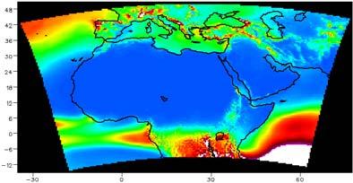
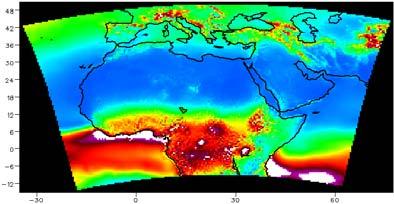
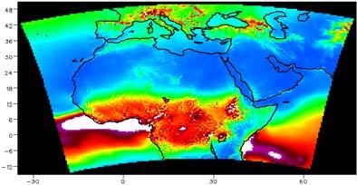
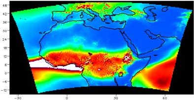
27 CRU ( ) Q0 Baseline ( ) June May April March February January 27

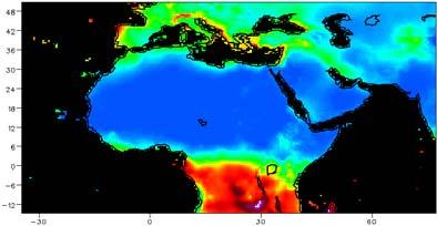
28 December November October September August July Figure 3.2 Simulated Baseline Precipitation for Q0 vs. CRU Data (mm/mon) 28

29 3.2 Projected Changes Temperature Figure 3.3, Figure 3.4, and Figure 3.5 compare the temperature between the baseline and future periods for Q0, Q2, and Q6 respectively. As can be seen, there is a consensus among the three scenarios on temperature increase over the whole domain and especially over the Arabian Peninsula in the summer months. The differences between the three scenarios are generally small. 29

30 Baseline Future June May April March February January 30

31 December November October September August July Figure 3.3 Simulated Baseline and Future Mean Temperature for ( K) Q0 31

32 Baseline Future June May April March February January 32

33 December November October September August July Figure 3.4 Simulated Baseline and Future Mean Monthly Temperature for ( K) Q2 33

34 Baseline Future June May April March February January 34

35 December November October September August July Figure 3.5 Simulated Baseline and Future Mean Monthly Temperature ( K) for Q6 35