Implementation of Estuary-Shelf Freshwater Exchange Parameterizations in the Community Earth System Model
|
|
|
- Linda Tucker
- 5 years ago
- Views:
Transcription
1 SciDAC: Collaborative project: Improving the Representation of Coastal and Estuarine Processes in Earth System Models th Annual CESM Workshop Implementation of Estuary-Shelf Freshwater Exchange Parameterizations in the Community Earth System Model Yu-heng Tseng (NCAR),Qiang Sun (U Connecticut), Michael Whitney (U Connecticut), Parker MacCready (U Washington), Frank Bryan (NCAR) Why? Estuary-Shelf Freshwater Exchange Parameterizations Improved augmented precipitation scheme Estuary and shelf box models Conclusion and Future


2 Coastal zone: coupled Air-land-ocean processes Multi-scale dynamics Johannessen & Macdonald (2009) Virtual salt flux: is it correct to consider the global water budget? Where are the impacts of costal ocean? Can we better represent the processes in the ESM (e.g., CESM)?


; 2 Yankovsky")
3 Improved augmented precipitation approach Empirical method Tseng et al. (2014 submitted) CESM OCEAN Wind-mixing plumes 3 Shelf break Buoyancy-driven plumes 24 Shelf Box Box Model Approach -Estuary box -Shelf box Estuary Box 1 River CESM SURFACE RUNOFF 1 Garvine and Whitney (2006); 2 Yankovsky and Chapman (1997); 3 Lentz (2004); 4 O Donnell (1999)
4 Two-layer Estuary Box Model Methodology Steady-state Governing Equations: Water mass flux conservation Salt mass flux conservation Potential energy flux (PEF) conservation SS uu ρρ uu QQ uu Estuary Box CESM POP Shelf Box ρρ rr QQ rr CESM Land SS ll ρρ ll QQ ll Tidal mixing and exchange

5 Off-line Estuary Box Model-validation with observation RR 2 = 64.14% RR 2 = 63.43%
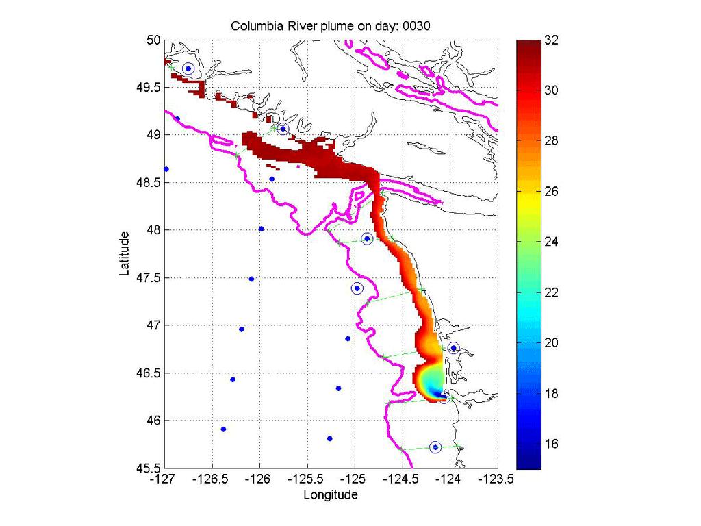
 CESM surface ocean salinity and velocity vector (annual mean) no Estuary Box Model output with Estuary Box Model output Columbia River")
6 Interactive Estuary Box Model (coupled with POP) Apply Box Model in the CESM ( CESM surface ocean salinity and velocity vector (annual mean) no Estuary Box Model output with Estuary Box Model output Columbia River Columbia River

7 Amazon CTR_e 1000 _r 300 CTR With EBM PHC CTR_e 1000 _r 300 -PHC CTR-PHC With EBM-PHC Summary of the estuary box model The estuary Box Model agrees well with observation in the Columbia River estuary. Surface salinity distribution at river mouth is obviously improved with estuary Box Model, but we need to introduce the shelf Box Model for more realistic salinity distributions on the shelf ocean.

8 Off-line Shelf Box Model-validation with ROMS
9 Conclusion and future The estuary box model is implemented and tested for Amazon and Columbia (offline and online coupled with POP) Parameters for different rivers are being estimated and examined (Congo and Mississippi rivers are done!) Top 20 rivers will be included and analyzed/compared The model framework of shelf box model is completed. It will be included and tested soon after the offline validation is completed (2014 summer) Validation/generalization ready for CESM2 (2014 winter)


10 Improved augmented precipitation Sensitivity of different h e on the surface salinity h e 30-year g40 average surface salinity. Columbia
 Enhanced MLD Similar improvement in the coupled b40 simulation than the g40 simulation but the magnitude is larger (due to a larger bias) Impacts are mostly local and influenced by")
11 Significant improvement in MLD Summary of the global impacts mixed layer depth (MLD) A reduction of ~8% of the surface salinity biases in coastal region Main improvement occurs in April-June (~12% in g40 simulation) Enhanced MLD Similar improvement in the coupled b40 simulation than the g40 simulation but the magnitude is larger (due to a larger bias) Impacts are mostly local and influenced by the nearshore circulation (largest when h e is comparable with the MLD), except the Arctic
12 Estuary Box Model Detail in Poster 189 Whitney Methodology Shelf Box A two-layer box with assumptions: Steady state and zeros net flux through the surface. SS uu ρρ uu QQ uu SS ll ρρ ll QQ ll Governing equations: Water mass flux conservation: ρρ rr QQ rr + ρρ ll QQ ll ρρ uu QQ uu + mm tt QQ uuuu ρρ ll ρρ uu = 0 Upper layer Lower layer CESM Land ρρ rr QQ rr Salt mass flux conservation: SS ll ρρ ll QQ ll SS uu ρρ uu QQ uu + mm tt QQ uuuu SS ll ρρ ll SS ll ρρ uu = 0 Potential energy flux (PEF) conservation: PPPPFF rr + PPPPFF ll PPPPFF uu + PPPPFF tt + PPPPFF tttt = 0 Color: Riverine water Oceanic water Estuarine water Mixing & exchanging


13 Off-line Estuary Box Model-validation with ROMS RR 2 = 60.38% RR 2 = 64.14%
14 Conclusion and future A simplified estuary-shelf freshwater exchange parameterization is developed based on an augmented precipitation method (i.e., the optimal Runoff effective depth, h R ) Locally improved simulation due to vertical mixing with little difference in a global view Further complicated parameterization based on Estuary and shelf box models


15 Why? How are these features affected by climate? Impacts of the nutrients and carbon from the river mouth Require better representation of transport and mixing processes along the coast - >help the global simulation Human impacts: 40% population lives along the coast


16 Why? Salinity bias Griffies et al. (2005) river discharge thickness hr=40 m -> hr=10m COREII forc. 1 POP Salinity (WOA09 annual mean) Larger bias in CCSM4 CCSM4 1 20th Century Ens. #1 ( )
=Δρgz Optimal Runoff effective depth (h R ) comparing")
17 Improved augmented precipitation scheme Actual river PE inputs often form slender coastal currents/plumes. Redistribute the runoff flux as a source term vertically by considering the change of available potential energy (APE)=Δρgz Optimal Runoff effective depth (h R ) comparing with the PHC3 Runoff effective depth h R can be determined by observation
18 A reduction of ~8% of the surface salinity biases in coastal region main improvement occurs in April-June (~12% in g40 simulation) Impacts are mostly local and influenced by the nearshore circulation. Global (65N south) ERR/RMS ERR (Annual mean) Arctic (65N north) ERR/RMS ERR (Annual mean) Coastal ERR/RMS ERR (Annual mean) Coastal ERR/RMS ERR (Jan-Mar) Coastal ERR/RMS ERR (Apr-Jun) Coastal ERR/RMS ERR (Jul-Sep) Coastal ERR/RMS ERR (Oct-Dec) g40 control 0.068/ / / / / / /0.819 g40 r150 control / / / / / / /0.841 g40 opt / / / / / / /0.813 b40 control / / / / / / /1.345 b40 r150 control / / / / / / /1.353 b40 opt / / / / / / /1.333


19 Vertical profiles averaged over W, N Salinity Temperature Density Diffusivity


20 Sensitivity of different h R on the surface salinity Amazon


21 Arctic Large warm bias cannot be corrected
22 Amazon Changjiang Columbia Ideal age in the coupled simulations


23
 height=4(m) MacCready et al.")
24 Estuary Box Model Comparison with 3D numerical model (ROMS) Box Model: Length=220 (km) Width=2.41 (km) height=4(m) MacCready et al. (2009) Estuarine Bathymetry NOAA Bonneville Dam ROMS: 246 horizontal grids 40 vertical layers
25 How? Estuary and shelf box model Salt and temperature fluxes Mixing φ = g 0 h ( ρ ρ)zdz h o dφ A = ΩBuoyant + ΩHeatflux + ΩTidal + ΩWind dt Approach by Garvine and Whitney (2006), Hordoir et al. (2008)
26 Shelf Box Model Methodology Buoyancy-driven situation Upwelling wind driven situation Wind relaxed situation V01 V01 CESM Land V01-V01 V01-V01 V01-V01