3.2.3 Groundwater Simulation. (1) Purpose

Transcription

1 The Study on Water Supply Systems in Mandalay City and in the Central Dry Zone Part II Study for Mandalay City Groundwater Simulation (1) Purpose Because the Central Dry Zone, Myanmar, including Mandalay City, has one of the least amount of precipitation in the southeastern Asia, the groundwater recharge rate is also presumed to be lower. Therefore, groundwater modeling studies are indispensable in order to design an optimal groundwater management plan for sustainable use of groundwater resources in Mandalay City. In Mandalay City, the groundwater resources have extensively been exploited to supply domestic and industrial water. The main well field including the Mandalay Water Supply System is located in the vicinity of the Ayeyarwaddy River, or in the western side of Mandalay City, and new well field is now needed to be constructed in southern part of the city. In the past, however, appropriate hydrogeological and groundwater modeling studies have not been carried out in the groundwater development in and around Mandalay City. For example, the well sites were simply selected without analyzing groundwater balance, and well yields were determined only by the results of pumping tests of each well. Groundwater development projects which ignore the groundwater balance could cause various kinds of groundwater problems: decline of groundwater levels in the wide area of Mandalay City, interference of wells, and saline or high hardness water intrusion from depths. Groundwater modeling techniques are world-widely adopted for many groundwater basins to investigate present groundwater flow condition including the groundwater balance, as well as to evaluate the amount of groundwater resources. The results of groundwater simulation will contribute to reveal groundwater potential quantitatively, and to establish groundwater development and/or groundwater management strategies. Therefore, the Study Team decided to perform groundwater simulation to evaluate present groundwater flow situation, and an optimal and sustainable pumpage for the groundwater development plan in Mandalay City. (2) Mathematical Model Groundwater models are representations of reality and, if properly constructed, can be valuable predictive tools for management of groundwater resources. That is to say, using a groundwater model, it is possible to test various management schemes. Groundwater models are divided into three categories: sand tank models, analog models and mathematical models. A mathematical model consists of a set of differential equations that governs groundwater flow, and is solved analytically or numerically. Since the 1960 s, when 2-118

2 The Study on Water Supply Systems in Mandalay City and in the Central Dry Zone Part II Study for Mandalay City high-speed digital computers became widely available, numerical models have been the favored types of model for studying groundwater. In this study, a numerical model using a digital computer is used. The goal of groundwater modeling is to predict the groundwater flow behavior against the effects of certain actions. However, before a predictive simulation can be made, the model should be calibrated and verified. This is because the validity of the predictions will depend on how well the model approximates field conditions. Additionally, groundwater modeling and calibration require overall knowledge not only on hydrogeology but also on socio-economic factors such as historical and existing groundwater use. (3) Simulation Program and Governing Equation As the simulation program, the MODFLOW is used in the Study. The program is developed by the United States Geological Survey (USGS), and is widely utilized for groundwater flow simulation throughout the world. The program adopts the following partial-differential equation to describe three-dimensional and constant density groundwater movement through porous earth media (Anderson & Woessner 1) (1992)), because groundwater flows three-dimensionally in a groundwater flow system: h Kxx + x x h Kyy y y + h h Kzz = Ss R * z z t ( ) where, Kxx, Kyy, and Kzz are values of hydraulic conductivity tensor along the x, y, and z coordinate axis, (LT -1 ); h is the hydraulic head (L); Ss is the specific storage of the porous media (L -1 ); t is time(t) ; and R* is sinks and sources of groundwater, which represents groundwater volume flowing into an aquifer in unit time and volume (T -1 ); Generally, Kxx, Kyy, Kzz and Ss may be functions of space (Kxx=Kxx(x,y,z) etc. and Ss=Ss(x,y,z)) and R* may be a function of space and time (R* = R* (x,y,z,t)). Equation ( ) describes groundwater balance under transient condition in a heterogeneous and anisotropic medium. The Modflow uses the finite difference method to solve the equation. (4) Required Parameters and Boundary Conditions The MODFLOW program requires the following hydrogeologic parameters: Top and bottom elevations of each aquifer 1) Anderson, M.P. and Woessner, W.W. (1992): Applied Groundwater Simulation of Flow and Advective Transport, Academic Press Inc

3 The Study on Water Supply Systems in Mandalay City and in the Central Dry Zone Part II Study for Mandalay City Aquifer Constants (effective porosity, specific storage, storage coefficient, horizontal hydraulic conductivity, transmissivity, and vertical hydraulic conductivity etc.) Initial groundwater levels Groundwater recharge rate Pumping rate from each grid and layer It is also needed to specify following parameters for groundwater simulation: Time dependence (steady-state or unsteady (nonequilibrium)) Duration of simulation and the time step Control parameter for numerical analysis Moreover, the following boundary conditions must be specified taking the actual hydrogeological situations into account: Constant head boundary including river boundary No flow boundary Drain boundary, general head boundary, etc. (if necessary) These parameters are analyzed and compiled in the next section. (5) Outline of the Model Aquifer unit classification, model structure, boundary conditions and some aquifer constants were specified as follows: 1) Aquifer Classification Judging from the available existing data, the Mandalay aquifer system consists of three aquifers and two aquitards (See 1.3 for the detail.). The 1st Aquifer is phreatic, or unconfined, and is composed of the Holocene sediments underlain by clayey formation. Although the detail data is not available about this clayey formation, the layer could be an aquitard overlying the 2nd Aquifer. The 2nd and 3rd Aquifers are main aquifers in Mandalay Area, and consist of the Pleistocene sediments. Most of the 2nd Aquifer and all of the 3rd Aquifer are under confined conditions. These confined aquifers are separated by a confining layer of hard clay (In the existing reports, the clay is sometimes expressed as shale ). Clayey sediments, Neogene sediments and Pre-Cretaceous rocks, which form hydrogeologically impermeable basements for the Mandalay aquifer system, underlie the 3rd Aquifer. 2) Model Structure Taking the hydrogeological information of Mandalay area into account, the structure of the simulation model was determined to be three-dimensional (3-D) model having

4 The Study on Water Supply Systems in Mandalay City and in the Central Dry Zone Part II Study for Mandalay City layers. Each model grid is 1km square in size. The modeled domain has 26 km in E-W direction and 35 km in N-S direction. cells are (601 meshes) (4 layers)= 2404 cells. The total number of active cells and river Because much information about the 1st Aquifer is not obtained, and for the simplicity of the model, the phreatic aquifer and the first aquitard were compiled to one layer taking the anisotropy into account. The classification of the hydrogeology is as follows: st Layer: (1st Aquifer Aq1 + 1st Aquitard Co1): Phreatic (Unconfined)/1st Aquitard nd Layer: (Shallow Confined Aquifer: Aq2): rd Layer: (2nd Aquitard: Co2): th Layer: (Deep Confined Aquifer: Aq3): 3) Boundary Conditions Confined (partially unconfined) Confined Confined Based on the hydrogeological structures of Mandalay Area, boundary conditions for st Layer were assigned as follows: Western and southern boundaries: Constant head boundaries were assigned at the Ayeyarwaddy and the Dotehtawaddy Rivers. For the constant head, the water level data at the river gauging stations were utilized. Eastern boundary: Where impermeable old rocks crop out, no flow boundary was given. While constant head boundaries were set at the apexes of alluvial fans. Northern boundary: Generally, groundwater flows from mountainside to the lowest place (in most cases, the largest river) in a groundwater flow system depending on the topography. Therefore, in natural conditions, east-to-west groundwater flow dominates in Mandalay Area. Since no flow crosses flow lines, a flow line can be treated as no flow boundary (Rushton and Redshaw 2) (1979)). In addition, several monadnocks composed of impermeable rocks exist some 10km northeast of Mandalay urban area. boundary. Therefore, no flow boundary was set at the northern Additionally, the effect of the Kandawghi Lake and the Thaung Tha Man Pond was taken into account. For nd and rd Layers, no flow boundaries were assigned based on the following reasons: Northern boundary is located on the flow lines. Further, the existence of several monadnocks suggests that the impermeable basement is shallow around the monadnocks. 2) Rushton, K. R. and Redshaw, S. C. (1979): Seepage and Groundwater Flow, John Wiley & Sons Inc., p

5 The Study on Water Supply Systems in Mandalay City and in the Central Dry Zone Part II Study for Mandalay City Western and southern boundaries are located under the Ayeyarwaddy and the Dotehtawaddy Rivers, respectively, which is thought to be the discharge area of the Mandalay groundwater flow system. Eastern boundary abuts on impermeable old rocks. (6) Input Parameters The calculation parameters for the MODFLOW program mentioned earlier were prepared based on the hydrogeological data. Followings are the initial input data obtained so far. Table indicates the summary. 1) Top and bottom elevations of each layer Top and bottom elevations of each layer are compiled from the existing geological columns (Fig.1.2.2) and electrical prospecting data conducted by the JICA Study Team (see Fig ). Geologic logs of newly drilled wells (PTW-28, JICA No.1 to 6, see 1.2.) are also utilized. 2) Aquifer Constants Table shows the aquifer constants. Most of the constants were mainly analyzed in this Study. Some of the constants, however, were compiled from pumping test results obtained by Ministry of Home & Religious Affairs 3) (1984) and MCDC 4) (1989) for the high resistivity zone of the electrical prospecting (See 3.2.1). In the model calculation, the aquifer constants in Table were applied using following assumptions: For effective porosity, 0.25 and 0.06 were given to sand and gravel, and silt and clay, respectively, based on Todd 5) (1980, pp.38). ) Specific storage is given as (storage coefficient)/(aquifer thickness). ) Ist Layer is mainly composed of fine sand (K=2.5m/d, S=0.1), and silt and clay (K=0.08m/d, S=0.06). [Values in the parenthesis are based on Todd (1980, pp.71).] In the initial model, the horizontal and vertical averages were used, and the aquifer constants were changed depending on the results of the simulation. ) The vertical hydraulic conductivities were analyzed using Hantush s method for leaky aquifer (see e.g. Walton 6) (1970).). The results are as follows (see also Fig ). For confined aquifers Aq2 and Aq3, anisotropy was thought to be negligible: Lower part of st Layer(Co1): m/day, rd Layer(Confining Layer): m/day 3) Ministry of Home & Religious Affairs (1984): Mandalay Water Supply Project, Design Concept Report, Report No.7/84. 4) MCDC (1989): Mandalay Water Supply Project, Hydrogeological Report on Mandalay City Area. 5) Todd, D.K. (1980): Groundwater Hydrology 2ed., John Wiley and Sons Inc., p ) Walton, W.C. (1970): Groundwater Resource Evaluation, McGraw-Hill, Inc., p

6 Well No. Table Aquifer Constants Year & Depth Screen Calculation Month Bored(m) Depth(m) Aquifer Method** T(m 2 /d) K (m/d)* S K '(m/d)* Notes Mar Shallow Jacob PW-1 Confined Theis (Aq2) Recovery Mar Jacob Theis Observation Well: PW-2 ditto Recovery PZ-2(r=20m) Recovery Hantush * Aq2 Average Geometric Mean Test Well Feb Deep Jacob ) Aquifer thickness Confined was assumed to be (Aq3) Recovery ) 20m. PTW-4 Feb Jacob * Observation Well: ditto Hantush * Test Well (r=110m) PTW-12 Dec Jacob ditto Recovery PTW-16 Feb Jacob ditto Recovery PTW-17 Mar Jacob ditto Recovery PTW-18 Feb Jacob ditto Recovery Aq3 Average Geometric Mean for high resistivity zone PTW-28 Aug Theis (0.306) ditto Jacob (0.331) Observation Well: Recovery Test Well (r=4.21m) Recovery PTW PTW-28 Average (Aq2:26.6, Aq3:42.6) JICA Theis (2.46) No.1 Oct ditto Jacob (2.84) Recovery Average (2.63) JICA Theis No.2 Nov ditto Jacob Recovery Average JICA Theis No.3 Nov ditto Jacob Recovery Average JICA-1 to 3 Average Observation Well: PZ-1(r=20m) Geometric Mean for intermediate resistivity zone Geometric Mean for low resistivity zone (all Aq3) * Aquifer constants from PTW-1 to PTW-18are mainly compiled from Ministry of Home & Religious Affairs(1984) and MCDC(1989). However, K,some data of S, and K ' are analysed in this Study. ** For details of the calculation methods, refer groundwater textbooks, e.g. Groundwater Hydrology by Todd(1980). Symbols) T: transmissivity, K : hydraulic conductivity(screen length was used as the aquifer thickness.), S: storage coefficient, K ': hydraulic coefficient of confining layer, r: distance between a pumping well and the observation well 2-123

7

8

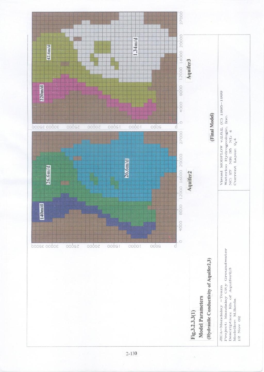
9 The Study on Water Supply Systems in Mandalay City and in the Central Dry Zone Part II Study for Mandalay City Additionally, a pumping test at well No.PTW28 near Mandalay Hill was carried out in order to estimate aquifer constants in the intermediate resistivity zone. Fig , Table and Table (1) in 2-D of Vol. III, Supporting Report, show the results. The hydraulic conductivity is about 37m/d, and is consistent with the resistivity. That is, the higher the resistivity indicates, the higher the hydraulic conductivity becomes except for impermeable rocks such as at Mandalay Hill. At PTW28, groundwater is drawn from two screens (12.6m) in the Deep Confined Aquifer (Aq3), and one screen (6.3m) in the Shallow Confined Aquifer (Aq2). For other wells, ratio of hydraulic coefficients (K) between the two aquifers is given by: K(Aq3): K(Aq2) = 1.6 : 1 ( ) At PTW28, { 2K(Aq3) + K(Aq2)}/3 = 37.3(m/d) ( ) If the relation ( ) is valid at PTW28, by solving the simultaneous equation the hydraulic conductivities are estimated as follows: K(Aq2) = 26.6m/d, K(Aq3) = 42.6m/d Thus, the aquifer constants are obtained both in the high and the intermediate resistivity zones of electrical prospecting (Refer to ). Therefore, it is desirable to obtain aquifer constants in the low resistivity zone as discussed in Fig also summarizes these constants for the initial model of the simulation. Table Input Parameters for the Groundwater Simulation Model (Initial Model) Model Layer Aquifer Unit st Layer (Aq1/ Co1) nd Layer (Aq2) 1st Aquifer/ 1st Aquitard Shallow Confined Aquifer Aquifer type Unconfined/ Confined Top and Bottom Elevation (masl) Top: 65 to 96 Btm: 45 to 72 Confined Top: 45 (partially to 72 Btm: -29 unconfind) to 47 Effective Porosity E E -05 SS Initial Recharge Heads Rate (masl) (mm/day) ± ( ) to ± ( ) to Pumping Rate (2002) (m 3 /day) rd Layer (Co2) th Layer (Aq3) 2nd Aquitard Confined Top: -29 to 47 Btm: -70 Deep Confined Aquifer Confined to +1 Top: -70 to +1 Btm: -95 to E to 7.2E ± ( ) to 42.6 to ± ( ) to *maslmeter above sea level,ssspecific storage, Kh and Kvhorizontal and vertical hydraulic conductivity respectively

10

11 The Study on Water Supply Systems in Mandalay City and in the Central Dry Zone Part II Study for Mandalay City 3) Initial Groundwater Levels and Changes in Groundwater and Surface Water Level As the initial groundwater levels for time-dependent simulation, calculated groundwater levels were estimated using steady-state simulation. For the calculated values, the continuous groundwater level measurement for 15 wells, and the simultaneous groundwater level measurement for 100 wells including river and pond water level were referred. Changes in groundwater level data of the deep confined aquifer have been observed only at 4 wells close to the Ayeyarwaddy River. The problem is that the data are dynamic groundwater level. Groundwater level data for other aquifers are not observed. Surface water levels corresponding to these well data are observed at Mandalay gauging station of the Ayeyarwaddy River. Close relationships between groundwater level of the deep confined aquifer and the river level are obtained (Fig ). 4) Recharge rate As discussed in (Groundwater Balance), average groundwater recharge rate in and around Mandalay City is estimated to be less than or equal to 1 mm/d (365mm/y). Further, as the recharge rate of the groundwater simulation, 0.84 mm/d (306mm/y) and 1.05 mm/d (383mm/y) were adopted for Mandalay urban area and the surrounding area, respectively. (7) Model Calibration Using Steady-State Calculation Before predictive simulation is conducted, the model was calibrated using steady-state calculation. Fig and Fig show some of the model parameters and cross sections respectively. The calibration results are shown in Fig and in2-d of Vol. III, Supporting Report, and are summarized in Table Table Comparison of Calibration Models Item & Case Case 1(initial model) Case 2 Case 3(final model) Payandaw River Not considered Considered Considered Ponds near Yangin Hill Not considered Considered Considered Constant Head Boundary Piedmo nt Fans Considered for large Hydraulic conductivity of Aquifer1 Hydraulic conductivity of Aquifer3 Result (* shows the maximum difference between observed and calculated groundwater levels of Aquifer1) Considered up to Considered up to small rivers intermediate rivers rivers Kh1(m/d) Assign higher (Constant) Kv1(m/d) value at piedmont fans (Constant) Kh3(m/d) Roughly assigned Assigned depending on the result of the electrical prospecting. *10m- Large difference is mainly caused by too low Kh1 & Kv1. * Figures for Cases 1 and 2 are shown in the Appendix *4m Improved. But, groundwater table is still higher in eastern Mandalay. And, it is lower in the Industrial Zone. Almost same as Case2. But, assigned higher value (42.6m/d) at southeastern Mandalay. *Almost fit. Along the Ayeyarwaddy River, depression of groundwater level in Aquifer 3 (main aquifer) was almost duplicated.

12 The Study on Water Supply Systems in Mandalay City and in the Central Dry Zone Part II Study for Mandalay City In the models, Kandawghi Lake, Thaung Tha Man Pond, and Tributary of the Ayeyarwaddy River were commonly considered as constant head boundary. Taking boundary conditions and hydraulic conductivities into account in detail, an almost fit model was obtained. From the calibration mentioned above, the followings are clarified: i) Average hydraulic conductivity of Aquifer 1 in both horizontal and vertical directions was estimated to be 2.5 and 0.08 m/d respectively. These values are consistent with those of fine sand, and silt and clay respectively. For groundwater recharge rate, estimated values from water balance (See ) are considered to be approximately valid. ii)along the Ayeyarwaddy River, groundwater depression in Aquifer 3 (main aquifer), which was found through the groundwater level measurement, was qualitatively duplicated. The depression is consistent with MCDC well field. This suggests that additional development of groundwater in this field is undesirable. Simulation parameters of the final model (Case 3) are summarized in Table In the next chapter, potential pumpage of groundwater in Mandalay will be estimated using the groundwater level obtained as the initial condition. Table Input Parameters for the Groundwater Simulation Model (Final Model) Model Layer st Layer (Aq1/ Co1) nd Layer (Aq2) Aquifer Unit 1st Aquifer/ 1st Aquitard Shallow Confined Aquifer Aquifer type Unconfined/ Confined Confined (partially unconfind) Top and Bottom Elevation (masl) Top: 65 to 96 Btm: 45 to 72 Top: 45 to 72 Btm: -29 to 47 Effective Poro-s ity SS (1/m) E E -05 Kh (m/day) Kv (m/day) Initial Heads (masl) ± ( ) to ± ( ) to 26.6 Recharge Rate (mm/day) 0.84(Man-dal y)to 1.05(Other area) Pumping Rate (2002) (m 3 /day) rd Layer (Co2) th Layer (Aq3) 2nd Aquitard Deep Confined Aquifer Confined Top: -29 to 47 Btm: -70 to +1 Confined Top: -70 to +1 Btm: -90 to E to 7.2E ± ( ) to ± ( ) to *maslmeter above sea level,ssspecific storage, Kh and Kvhorizontal and vertical hydraulic conductivity respectively. Bouwer, H. (1978): Groundwater Hydrology, McGraw-Hill, Inc., p.480. Wang, H.F. and Anderson, M.P. (1982): Introduction to Groundwater Modeling, Freeman, p

13

14

15

16

17

18